HAL Id: hal-01673738
https://hal.archives-ouvertes.fr/hal-01673738
Submitted on 31 Dec 2017
HAL is a multi-disciplinary open access
archive for the deposit and dissemination of
sci-entific research documents, whether they are
pub-lished or not. The documents may come from
teaching and research institutions in France or
abroad, or from public or private research centers.
L’archive ouverte pluridisciplinaire HAL, est
destinée au dépôt et à la diffusion de documents
scientifiques de niveau recherche, publiés ou non,
émanant des établissements d’enseignement et de
recherche français ou étrangers, des laboratoires
publics ou privés.
New Evidence Based on a New Data Set
Andre Gbato
To cite this version:
Andre Gbato. Impact of Taxation on Growth in Sub-Saharan Africa: New Evidence Based on a
New Data Set. International Journal of Economics and Finance, 2017, 9, �10.5539/ijef.v9n11p173�.
�hal-01673738�
Published by Canadian Center of Science and Education
Impact of Taxation on Growth in Sub-Saharan Africa: New Evidence
Based on a New Data Set
André Gbato1
1 Auvergne University, CERDI UMR CNRS 6589, France
Correspondence: André Gbato, PhD Candidate Auvergne University, CERDI, 65 Boulevard François Mitterrand 63000 Clermont-Ferrand, France. E-mail: [email protected]
Received: September 12, 2017 Accepted: October 14, 2017 Online Published: October 25, 2017 doi:10.5539/ijef.v9n11p173 URL: https://doi.org/10.5539/ijef.v9n11p173
Abstract
In this study, we empirically test impact of taxation on long-run growth of a sample of 32 countries in sub-Saharan Africa. The results indicate a zero effect of taxation on long-run growth. Moreover, the results suggest a significant negative effect of indirect taxes and taxes on individuals in short term. Consequently, the use of taxation as an instrument of intervention is not appropriate in the region. The countries of the region could therefore increase their growth, if the design of fiscal policy rests solely on logic of fiscal neutrality.
Keywords: growth, taxation, heterogeneous panels, cross-sectional dependence 1. Introduction
Taxation in developing countries is a strategic tool of the highest order. It makes it possible to finance the provision of public goods such as infrastructure, education, health and justice, which are essential for growth. But beyond that, taxation affects individual savings, work and education decisions; production, job creation, investment and business innovation; as well as the choice of savings instruments and assets by investors (OECD, 2009). All these decisions are affected not only by level of taxes, but also by way in which different fiscal instruments are designed and combined to generate government revenues.
In Sub-Saharan Africa, taxation is perceived as a brake on growth. Taxes rules are insufficiently tailored to the taxpayer’s specificity, and very often do not take into account the weak administrative capacity available in the countries of the region. Faced with this situation, countries in the region have embarked on reforms aimed at alleviating the burden of tax structures that hamper economic growth. These reforms are generally aimed at creating a tax environment that encourages savings, investment, entrepreneurship and labor. They are not necessarily aimed at lowering the tax burden but seek to redefine the tax structure that would minimize the negative impact of taxes on growth while preserving fiscal revenues. In practice, these reforms have introduced tariff and tax rate reductions that have not always succeeded in widening the domestic tax base.
In this context, economic growth in the region has slowed significantly in recent years. It fell to 3.4% in 2015, its lowest level in the past 15 years, and could continue to slow to 1.6%, namely well below the rates of 5% to 7% recorded during the past decade (IMF, 2016). For countries in the region, that prioritize fiscal policy as an instrument of intervention, this situation revives the debate on the role that tax policy could play. The crucial issue is: is tax policy can improve growth?
To the extent that African countries have embarked on poverty reduction strategies, which will lead to significant recurrent costs, and with revenue losses caused by the increasing liberalization of economies, it is important that domestic revenues be higher to prevent a rapid increase in public debt. It is also essential to reduce negative externalities of taxation on economic growth so as not to hamper development. These two imperatives require construction of tax system which is both income-generating and growth-friendly. This raises another question: is there a beneficial tax structure to growth?
To answer these questions, it is necessary to analyze experience of sub-Saharan African’s countries. The main objective of this study is therefore to evaluate empirically the impact of taxation on economic growth of sub-Saharan African’s countries (SSA), using the DCCE approach of Chudik and Pesaran (2015) on period 1980-2010. More specifically, the study explores the relative impact of different components of tax revenues on economic growth. Few studies have analyzed the influence of different tax instruments on the growth of SSA
countries. One reason for the limited number of empirical studies on the subject in the region has been the lack of reliable data on taxation, including the various components of tax revenues. But this gap was filled by Mansour (2014). Using this data, the paper marginally contributes to empirical literature, showing how different types of taxes specifically affect growth in SSA, distinguishing between resource-rich and resource-poor countries.
The rest of this article includes 5 sections. After a brief presentation of the African tax policy, we review the theoretical and empirical results on taxation and growth. We then present a framework for methodological analysis before presenting and discussing the results.
2. Tax Policy in Sub-Saharan Africa 2.1 Evolution of Different Tax Revenues
Tax revenues (Note 1) have evolved in recent years (see Figure 1). On average, they increased from 12% in 2000 to more than 15% of GDP in 2010. This reflects an increase in revenue from consumption taxes and an improvement in direct taxes. Figure 2 shows the annual average of indirect taxes (denoted IC) and direct taxes in shares of total non-natural resource tax revenues. Overall, indirect taxes are the dominant force in tax revenue. This is not surprising, given that since its introduction in the 1990s, VAT has met with success in the countries of the region. The ease of implementation and the low economic cost of VAT have favored the mobilization of significant revenues. Thus, the share of indirect revenues in the countries studied rose from 27% in 1990 to 43% of total tax revenues in 2010.
Figure 1. Evolution of tax revenue
Direct taxes have not grown as high as indirect taxes. From 27% in 1990 these taxes will decline to around 25% between 1991 and 1998. This decline coincides according to Mansour (2014) with the increase in revenues from natural resources in the same period. He argues that this decline is the result of a deliberate policy of substituting taxes on natural resources for direct taxes and of relaxing audit rules for companies and individuals. The reasons for this decrease could also be sought on investment incentives side. Indeed in many countries of the region the desire to attract foreign investment will lead to the creation of investment codes with numerous favors and tax exemptions. Most tax incentives have consisted of tax holidays (Note 2) and other instruments to reduce the effective rate of corporate tax. According to Cleeve (2008), these incentives have not been effective and have contributed to exacerbating problems related to governance and corruption. From 1999 onwards, direct taxes will increase to around 30% in 2010. This increase is marked by an increase in both personal income taxes (denoted IRP) and corporate taxes (denoted IS) (Figure 2).
Figure 2. Evolution of direct and indirect tax revenue as a percentage of tax revenue
12 13 14 15 16 T a x re ve n u e ( % GD P ) 1980 1990 2000 2010 year 20 25 30 35 40 1980 1990 2000 2010 year
Indirect indirect tax revenue (% Tax revenue) Indirect direct tax revenue (% Tax revenue)
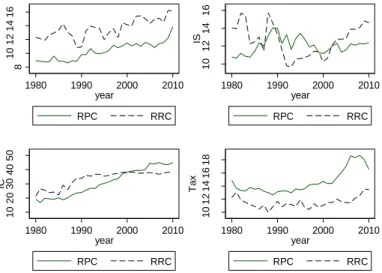
However, the evolution of tax revenues has not been uniform in the region. Analyzing revenue through the prism of natural resources weight in the rich countries, it appears a significant difference (Figure 3) in poor (RPC) and rich in natural resources countries (RRC (Note 3)). Since 1990, RPCs have mobilized more non-resourced tax revenues than RRCs. On the other hand, the share of indirect taxes in revenues was higher among RPCs. Conversely, the share of direct taxes in revenues was higher in the RRCs. On average, the share of internal indirect taxes was 45.7% for RPCs, compared with 37.6% for RRCs between 2000 and 2010. Personal and corporate taxes represented 15.6% and 13% respectively for RRC, while in RPCs they were 12% and 11.7%.
Figure 1. Comparison of revenue performance between RPC and RRC
Note. IS = Corporate tax revenues as a percentage of tax revenue. IRP = personal tax revenue as a percentage of tax revenue. IC = internal
indirect tax revenue as a percentage of tax revenue. Tax = tax revenue as a percentage of GDP.
2.2. Problem of Sub-Saharan Taxation
In sub-Saharan Africa, as in other developing countries, primary objective of fiscal policy is the mobilization of revenues. Faced with increasing costs and instability of external sources of development financing (Note 4), mobilization of adequate tax revenues, stable and predictable is as imperative to finance the provision of public goods. However, as in many developing countries, there are several difficulties in mobilizing revenues in the region. First, the low level of the wealth produced (Note 5) significantly limits ability to pay the debt. Indeed, Tanzi and Zee (2001) emphasize that the level of taxation follows the process of development and industrialization. Second, revenue mobilization is limited by the fact that the distribution of tax burden is not equitable (Tanzi & Zee, 2001). According to Itriago (2011), the bulk of the tax burden is borne by the underprivileged classes, under the action of privileged groups. Another problem stems from the lack of accountability in policies that creates a sense of injustice in the taxpayer. Bird, Martinez and Togler (2008) show that revenue mobilization increases with political accountability and the ability of taxpayers to sanction decision-makers. Unfortunately, in sub-Saharan Africa, this relationship is biased by foreign aid, often guided by geopolitical interests.
Faced with these different constraints, the countries of the region undertook various reforms. But without a clear and precise match between fiscal reforms and the development strategy, reforms are struggling to prove their effectiveness. Indeed fiscal policy is shared neutrality and interventionism, and between the redistribution of income and the promotion of economic growth. The ambiguity and diversity of the ends pursued thus constitute another brake on efficiency. While it is true that a high rate of growth associated with an equitable distribution of wealth is ideal, their reconciliation is difficult (Hamzaoui and al., 2017). A choice is therefore necessary and this requires answering the following question: greater equality, at prices of growth retardation is preferable?
Given the relatively low GDP of sub-Saharan economies, income redistribution brings relatively little to low-income groups, much less than what its advocates claim (Itriago, 2011). Charging the rich can be politically advantageous, but it does not improve the overall purchasing power. The solution to the problem of redistribution is based on an ethical choice regarding the importance to be attributed to income distribution and growth in the short and long term (Hamzaoui et al., 2017). Thus, taxation should initially encourage and
8 10 12 14 16 IRP 1980 1990 2000 2010 year RPC RRC 10 12 14 16 IS 1980 1990 2000 2010 year RPC RRC 10 20 30 40 50 IC 1980 1990 2000 2010 year RPC RRC 10 12 14 16 18 T a x 1980 1990 2000 2010 year RPC RRC
a policy of income redistribution that is likely to be that of poverty (Moummi, 2012). The goal of reducing inequality can only be achieved through relatively high and sustainable economic growth.
The search for strong and sustainable growth raises another question. Should taxation move towards more neutrality or more interventionism? In liberal developed countries, growth depends to a large extent on the dynamism of private enterprise. But in the developing world, the private sector remains weak. This deficiency in private enterprise necessitates State action, which must then replace the private entrepreneur (Hamzaoui et al., 2017). Therefore, budgetary choices become essential. The lack of resources and the size of the needs require some rationalization of budgetary choices. There is also a need to promote a fiscal policy that can mobilize significant resources. But since sustainable growth is based on an optimal allocation of production factors, it is important that taxation does not impede the optimal allocation of production factors. This implies that taxation is neutral from the point of view of social and economic incentives. However, very often this growth objective has been translated into sub-Saharan Africa (SSA), by a more complex tax regime due to tax exemptions or lower effective tax rates caused by tax competition between states. These changes influence either tax revenues or capital inflows and outflows. This in turn affects the economic growth of competing countries (Fayçal & Saloua, 2016).
This interventionism of the African States to revive the economy is incompatible with the search for neutrality, which is of capital importance according to Lauré (1953, 1957). First, because productivity’ gains are due to neutrality in relation to the production process and the division of labor. Second, the neutrality with respect to the formation of prices of goods and factors of production, expresses the real economic rarity: it is therefore necessary to avoid that the tax levies bias this system of prices, at the risk of arriving at suboptimal decisions. Finally, neutrality in relation to the factor of production avoids waste in terms of capital.
3. Literature Review 3.1 Theoretical Predictions
The relationship between fiscal policy and economic growth has found a wide scope in the growth literature. However, the theoretical study on the effect of fiscal policy on economic growth is still inconclusive (Tosun & Abizadeh, 2005).
The neoclassical growth models of public policy (see, for example, Judd, 1985, Chamley, 1986) give fiscal policy the role of determining the level of output rather than the long-term rate of growth. The equilibrium growth rate is based on exogenous factors such as population growth and technological progress, whereas fiscal policy can only affect the process of transition to this state of equilibrium. On the other hand, models of endogenous public policy growth (see Barro & Sala-i-Martin, 1992; Stokey & Rebelo, 1995; Mendoza et al., 1997) provide mechanisms by which fiscal policy can determine both the level of Production and growth rate at equilibrium. These endogenous growth models suggest that taxation can have a negative effect and a positive effect on the growth rate. The positive effect is indirectly driven by tax-financed spending.If taxes are used to finance investments in public goods, especially goods generating positive externalities (infrastructure, education and public health), economic growth rate can be positively influenced by taxation. The negative effect of taxation on growth stems from the modification of individuals’ decisions in the direction of sub-optimality. Engen and Skinner (1996) suggest five possible mechanisms by which taxes can affect economic growth: (1) the rate of investment may be hindered by taxes such as corporate and personal income and capital gains taxes;(2) taxes can slow the growth of labor supply by distorting leisure and leisure choices; (3) tax policy can affect productivity growth through its discouraging effect on research and development (R&D) spending;(4) taxes may result in a flow of resources to other (less taxed) sectors likely to have lower productivity;and (5) high taxes on labor supply can distort the efficient use of human capital by discouraging workers from jobs with high tax burdens.
3.2 Empirical Work
3.2.1 General Works
Empirically, studies on taxation’s impact have been approached in different ways, leading to different results. Miller and Russek (1997) applied panel’s method to data from 39 countries of different development levels (developed and developing countries) over period 1975-1984. First, they find a positive correlation between corporate tax revenues and economic growth using the total sample. Second, they do not find a significant relationship between the taxation of domestic consumption and growth.In the case of developed countries, there is a negative correlation between the taxation of personal income, social security contributions and growth.For developing countries, they find a positive correlation between corporate tax and personal tax on the one hand,
and economic growth on the other.
Kneller Bleaney and Gemmell (1999) estimate effects of different taxes on a panel of 22 OECD countries between 1970 and 1995. They differ in their study of the taxes-distorting (Note 6) and neutral tax (Note 7), as well as other elements of the budget. Their pooling and fixed effects estimates suggest that a higher level of distorting taxes (as a ratio of total GDP) reduces per capita income. Nevertheless, the baseline results are not robust when the authors use the instrumental variable estimation to address the potential endogeneity of the tax variables.
Widmalm (2001) using Leamer extreme bond analysis, showed data from 23 countries over the period 1965-1990 that the tax on personal income has a negative impact on growth Unlike the consumption tax. Lee and Gordon (2005) found the corporate income tax rate to have a negative impact on growth by applying the panel estimation method to data from 70 developed and developing countries over the period 1980-1997.
Angepoulos, Economides and Kammas (2006) find that the taxation of labor income has a negative impact on growth, while corporate tax and capital income tax have a positive impact on growth. They find these results by applying the panel’s method to a sample of 23 OECD countries.
Arnold (2008; 2011) uses an error correction panel on data from 21 OECD countries over the period 1970-2005. He finds that taxes on wealth, and in particular periodic taxes on real estate, are the most favorable to growth, followed immediately by taxes on consumption. Individual income taxes are significantly less favorable, and corporate income taxes have the most negative effects on GDP per capita.
Xing (2012) uses an empirical analysis based on the error correction model data from OECD countries. First, it finds that the personal income tax, the corporate income tax or the consumption taxes are associated with a lower per capita income level in the long term.He concludes that in order to promote growth, there is no evidence that personal income taxes are better than corporate income taxes, or that consumption taxes are better than income taxes.
Santiago and Yoo (2012) analyzed 69 countries ranked among high-income, middle-income and low-income countries over the period 1970-2009. It uses an error correction model for this purpose. First they find that income taxes, social security contributions and personal income taxes have a strong negative association with growth as corporate income taxes. Then they find that the property tax has a strong positive association with growth. Finally, a reduction in income taxes and an increase in value added taxes on sales are also associated with faster growth. However, they report that their results are applicable to high-income and middle-income countries, but not to low-income countries.
Mehrara, Masoumib, and Barkhi (2014), looking at the effect of fiscal policy on economic growth and inflation, find that using the PVAR approach a shock in tax revenues in the short term Long-term economic growth has no effect on growth. They also find that indirect taxes have more effect than other types of taxes at the macroeconomic level.Their analysis is based on a sample of 14 developing countries over the period 1990-2011. Hakim, Karia and Bujang (2014) examine the impact of indirect taxes, especially VAT, on economic growth in developing and developed countries using the Arellano-Bond GMM estimator. They find that indirect taxes are negatively correlated with economic growth in developing countries, and significantly and positively correlated with economic growth in developed countries. They conclude that the implementation of the current flat rate VAT is less effective in raising higher revenues and stimulating growth in developing countries. The implementation of current VAT should therefore be revised in order to generate higher revenues and economic growth without seriously affecting the consumption and real per capita income of developing countries.
Arachi, Bucci and Casarico (2015) studied the relationship between growth and tax structure using implicit tax rates and tax ratios as indicators.They apply for these estimator common effects correlated (Note 8) on a sample of 15 OECD countries from 1965 to 2011. They found that the link between tax structure and long-term per capita GDP is not robust when the hypothesis Unobservable heterogeneity between countries is adopted.These results are confirmed by Baiardi, Profeta, Puglisi and Scabrosetti (2017).
Overall, this work resulted in various and sometimes contradictory results depending on the period or sample. Apparent contradictions can be attributed to the different econometric methodologies used, and to the characteristics specific to different economies during alternative periods.Moreover, most of the work concerned OECD countries. As a result, the results of these analyzes can’t be generalized to all other countries and especially to SSA countries. The debate on the relationship between fiscal policy and growth therefore remains open and requires further investigation.
3.2.2 Sub-Saharan Africa Specific Work
Various empirical studies have investigated the effects of taxes on economic growth. The results are far from conclusive, varying according to the countries, the methodologies and the tax variables involved. This section presents earlier empirical work on African countries.
Keho (2010) who adopted the Scully regression models and quadratic concludes that higher taxes are strongly correlated with reduced economic growth in Cote d’Ivoire. A similar negative relationship between the tax burden and the economic growth rate in Nigeria and South Africa was reported by Saibu (2015).In another study Keho (2013) adopting the linear programming methodology of Branson and Lovell (2001) finds that higher taxes are associated with reduced economic growth.
Wisdom (2014) applied Granger’s cointegration and causality tests and found that tax revenues had a positive and statistically significant impact on Ghana’s economic growth both in the long term and in the short term. Sekou (2015) in his study uses the ordinary least squares method, and reports a significant and positive correlation between tax collection and growth in Mali. Chigbu et al. (2011), Ogbona and Appah (2012), and Confidence and Ebipanipre (2014) found similar results. Their results suggest that tax reform is positively and significantly related to economic growth in Nigeria.
Keho (2011) finds that there is a long-term relationship between the different tax revenues with the exception of direct taxes and growth in Cote d’Ivoire. It finds a two-way causality between tax revenues and long-term production, which implies a virtuous circle of taxes and GDP. Direct taxes, however, did not cause GDP in the short and long term.These results suggest that tax revenues depend on economic activity, and reducing the tax burden from direct taxes to indirect taxes is likely to have a positive effect on growth.
Ugwunta and Ugwuanyi (2015) applied an estimate of panel data under the assumption of a fixed unobservable effect. They find that taxes on income, profits, capital gains, taxes on payroll and labor, property taxes, estates, fixed assets and financial transactions have a negative and insignificant effect.On the other hand, indirect taxes have a positive and insignificant effect on the economic growth of sub-Saharan African countries. A similar result was obtained by N’Yilimon (2014) using the unit root test on the panel data. He suggests that there is no non-linear link between taxation and economic growth in the West African Economic Monetary Union (UEMOA) countries. Dasalegn (2014), using the ordinary least squares method, finds that VAT receipts play a significant and positive role in the national development of Ethiopia. Edame and Okoi (2014), and Lawrence (2015) interested in the effect of VAT on economic growth in Kenya found a significant and negative relationship between the two variables.
4. Empirical Analysis
The empirical analysis is performed by estimating an error correction model specified as follows:
∆ ln 𝑌𝑖𝑡= −𝜑𝑖*ln(𝑌𝑖𝑡−1) − ∑ 𝛽𝑖 𝑗 ln(𝑋𝑖𝑡−1j ) 𝑗 − ∑ 𝛽𝑚 𝑖𝑚ln( 𝑇𝑖𝑡−1𝑚 )+ + ∑ 𝑏𝑖 𝑗 ∆ln(𝑋𝑖𝑡j) 𝑗 + ∑ 𝑏𝑚 𝑖𝑚∆ln(𝑇𝑖𝑡m) + 𝛾𝑖𝑧𝑡 + 𝛿𝑖+ 𝜀𝑖𝑡
Where ∆ is the first difference (replace with “D” in regressions’ results). Prefix “ln” refers to logarithm (indicate by “l” in regressions’ results). 𝑌𝑖𝑡 is real GDP per capita of country “i” at year “t”. 𝑋𝑖𝑡−1𝑗 represents investment in
physical capital. 𝑇𝑖𝑡−1𝑚 represents tax variables, i.e., total revenues as a percentage of GDP or tax revenues from internal taxes (corporate taxes, personal taxes and consumption taxes). Corporate taxes, personal taxes and consumption taxes are expressed as percentage of revenue following Arnold (2008; 2011), Xing (2012), Arachi et al. (2015), and Baiardi et al. (2017).
The variables 𝑧𝑡−1 and 𝛿𝑖 represent respectively the temporal effect and the individual effect specific to each
country. 𝜀𝑖𝑡 represents the term idiosyncratic error.
The parameters 𝛽𝑖𝑗 and 𝛽𝑖𝑚 represent the long-run equilibrium relationship between the logarithm of real GDP per capita, respectively, investment and fiscal variables. The parameters 𝑏𝑖𝑗 and 𝑏𝑖𝑚 capture the short-term
relationship between the logarithm of real GDP per capita, respectively, investment and fiscal variables. The parameter −𝜑𝑖 indicates the economy’s speed of convergence to the long-term balance. The term in parenthesis represents the cointegration relationship as we seek to identify in our approach. To estimate the model, equation (1) can be rewritten as:
Long-term parameters 𝛽𝑖𝑗 and 𝛽𝑖𝑚 can be calculated from 𝜋𝑖𝑗 and 𝜋𝑖𝑚, as follows: 𝛽𝑖𝑗=𝜋𝑖
𝑗
𝜋𝑖𝑐; 𝛽𝑖 𝑚= 𝜋𝑖𝑚
𝜋𝑖𝑐 ; avec 𝜋𝑖𝑐 = −𝜑. Parameter 𝜋𝑖𝑐 gives an overview of the presence of a long-run equilibrium relationship: if 𝜋𝑖𝑐 = 0 there is no cointegration and model reduces to a regression with variables in first difference. Inversely if 𝜋𝑖𝑐≠ 0, variables in brackets of equation (1) have long-run relationship. In this case, after shock, the economy returns to its long-term equilibrium path.
To control for unobservable common shocks and for the omitted variables cointegration relationship, we follow the approach DCCE (Note 9) proposed by Chudik and Pesaran (2015) by including in regression the cross-section averages of all variables of the model. Equation (2) becomes:
∆ ln 𝑌𝑖𝑡= 𝜋𝑖𝑐ln(𝑌𝑖𝑡−1) − ∑ 𝜋𝑖𝑗 ln(𝑋𝑖𝑡−1 j ) 𝑗 − ∑ 𝜋𝑚 𝑖𝑚ln( 𝑇𝑖𝑡−1𝑚 )+ ∑ 𝑏𝑖𝑗∆ln(𝑋𝑖𝑡 j ) 𝑗 + ∑ 𝑏𝑚 𝑖𝑚∆ln(𝑇𝑖𝑡m) + 𝜋𝑖𝑐ln(Y̅̅̅̅̅̅̅̅̅̅ +t−1) ∑ 𝜋𝑗 𝑖𝑗ln(𝑋̅̅̅̅̅̅̅̅̅̅̅̅𝑖𝑡−1j )+ ∑ 𝜋𝑚 𝑖𝑚̅̅̅̅̅̅̅̅̅̅̅̅ln( 𝑇𝑖𝑡−1𝑚 )+ 𝑠𝑖 ∆ ln 𝑌̅̅̅̅̅̅̅𝑡+ ∑ 𝑠𝑗 𝑖𝑗̅̅̅̅̅̅̅̅̅̅̅∆ln(𝑋𝑖𝑡j)+ ∑ 𝑠𝑚 𝑖𝑚∆ln(𝑇̅̅̅̅̅̅̅̅̅̅̅𝑖𝑡m)+ 𝛾𝑖𝑧𝑡+ 𝛿𝑖+ 𝜀𝑖𝑡
Recent studies have shown that the DCCE is an effective method to overcome many difficulties. First, this method allows each country to have its own slope coefficients on both the observed explanatory variables and unobserved common factors. Then, DCCE is robust method for estimating non-stationary panels with different types of cross-dependencies errors (Eberhardt & Presbitero, 2013; Chudik & Pesaran, 2015). However, this approach may suffer a slight bias when the time dimension is moderate. To correct this bias, we apply to all estimates, the average readjustment recursive method proposed by Chudik and Pesara (2015).
The DCCE estimator may be invalid when the model to be estimated comprises a lagged dependent variable and / or weakly exogenous variables such regressors, as is the case in our model. In this case, Chudik and Pesaran (2015) show that the DCCE approach continues to be valid if a sufficient number of shifts average cross the model or additional control variables are included in the equation (3). Therefore, we follow this procedure to check the robustness of our results.
5. Data
Our sample comprises 32 SSA countries with a representation of RRC parity and RPC (Table 8). The data cover the period from 1980 to 2010. The sample design was guided by data availability. The investment is used as a proxy of capital. The data on real GDP growth rate per capita is taken from the World Bank database (WDI). The investment is taken from the IMF database (WEO, 2015). All fiscal variables are taken from the FERDI development indicators.
In order to perform robustness checks, we include in the empirical model two additional variables: trade openness, calculated as the sum of exports and imports to GDP, and a proxy public expenditure, calculated as the ratio of final consumption of general government in GDP. Proxies of trade openness and public expenditures are taken from the World Bank database.
6. Results
6.1 Cross-Sectional Dependence Test
Before starting the empirical analysis, data were subjected to analysis of the dependence in cross section. The independence of errors between individuals (correlation [ ] = 0) is an important property for the estimation
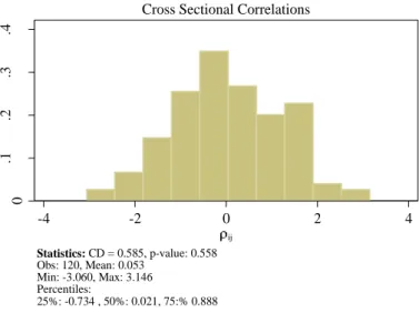
of panel data. When this hypothesis is violated, ordinary estimators are biased and inconsistent (Sarafidis & De Hoyos, 2006). Indeed, a strong dependency between errors greatly reduces the efficiency of the least squares estimator (Phillips & Sul, 2003) and makes estimates using instrumentation inconsistent variables (Sarafidis & Robertson, 2006). However when this dependence is relatively small, it does not need to be taken into account in the data analysis because its effect is negligible (Chudik et al., 2011). Thus, we test the dependence with the test proposed by Pesaran (2015). Under the null hypothesis of weak dependence, the test P-value is 0.00. The P-value is less than the 5% significance level which leads to reject the null hypothesis of weak dependence (Figure 4).
Figure 2. Cross section dependence test
6.2 Unit Root Test
Stationary is important property when you want to use the temporal dimension of macroeconomic variables. Unit root test provides information on stationarity of times series. Presence of unit root dramatically affects the asymptotic properties of tests and estimates temporal series (Granger & Newbold, 1974). The use of stationarity test avoids false regressions involving non-stationary variables. In this section we conduct unit root tests for panel data, since the individual unit root tests are known for their low power (Cochrane, 1991), especially if the time dimension is limited.
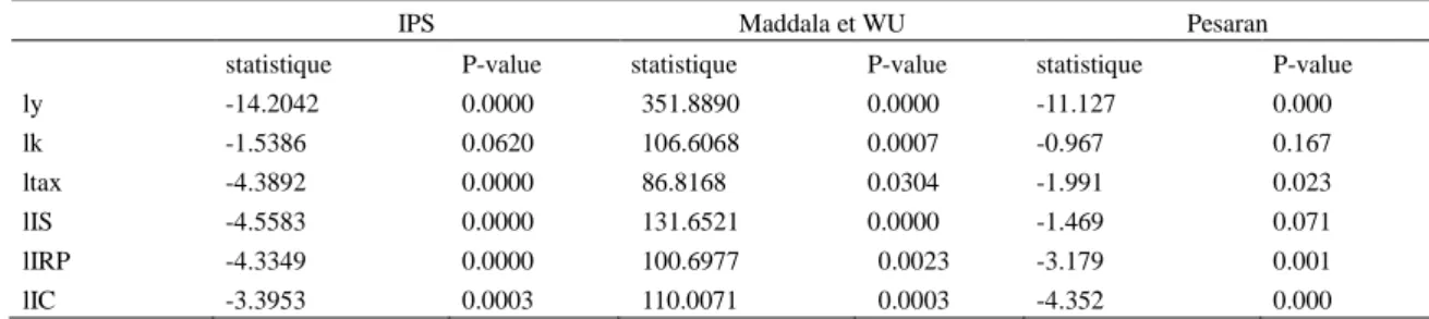
Validation of cross-sectional dependence in the data implies that the negligence of unobserved common factors could skew the usual unit root tests in panel. Due to some gaps in our data, we test the existence of unit root tests thanks to Choi (2001), Im, Pesaran and Shin (Note 10) (2003), of Maddala and Wu (1999) and Pesaran (2007). With the exception of test Maddala and Wu, other procedures offer the opportunity to reflect dependence of individuals. All tests are testing the null hypothesis of non-stationary against the alternative of stationary of the variables while providing the opportunity to consider the issue. The tests of Maddala and Wu (1999) and Choi (2001) are Fisher tests. They perform individually Dickey and Fuller test, and Phillips and Perron test. They then combine the P-value of individual unit root tests for the final statistics. However the test Choi (2001) is distinguished from the test Maddala and Wu (1999) by the use of alternative methods of combinations. Three methods differ according to whether they use the inverse transformation 𝜒2, the reverse-normal and reverse logit P-value, and the fourth method is a modification of the inverse transformation of 𝜒2 that is suitable when N approaches infinity. The normal and reverse inverse transformation logit can be used when N is finite or infinite. The IPS test combines the information of the size of the time series with that of the dimension of the cross section, so that less time observations are necessary for the test has the power. This procedure makes separate unit root tests for N cross sections. The final result of the test is based on the average of N statistics Dickey-Fuller Augmented (ADF). Pesaran unit root test (2007), still little known, is to estimate for each individual equation (4), and obtain the statistical Dickey-Fuller 𝜌𝑖. The final statistic, named CIPS (Note 11), is obtained by averaging the individual statistics Dickey-Fuller Augmented. The test provides a truncated version of the CIPS denoted CIPS*, to avoid any influence of extreme results that might occur for samples with low dimension T. The test results are shown in Tables 1 and 2. For all variables, the P-value is mostly below the 5% threshold. These results lead us to conclude that all variables are stationary.
6.3 Estimation
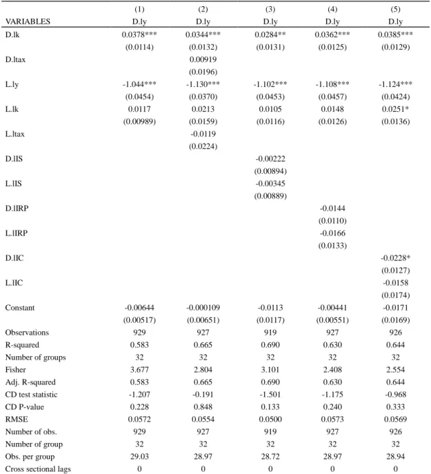
In this section we follow Presbitero and Eberhardt (2013) by testing the cointegration from estimator Chudik and al (2015). Table 3 summarizes baseline results (Note 12) of long-term and short-term factors estimation and the estimated speed of convergence between countries, from the DCCE estimator. In column 1, we regress the log of real GDP per capita on investment measures. In columns 2 to 5, we include tax variables. In columns 2 to 5, fiscal policy is successively measured by total revenue, followed by the various revenue components.
The results in Table 3 show that coefficient of lagged growth is negative and significant. In other words, deviation from the growth of its value predicted by the long-term relationship triggers a change in the growth in
0 .1 .2 .3 .4 Density -4 -2 0 2 4 ij Statistics: CD = 0.585, p-value: 0.558 Obs: 120, Mean: 0.053 Min: -3.060, Max: 3.146 Percentiles: 25%: -0.734 , 50%: 0.021, 75:% 0.888
the opposite direction in order to regain the level of long term. The results further suggest that the restoring force is around 1, which implies a growth of deflection takes about one year on average to reach its equilibrium level. The estimated coefficient of capital is positive and highly significant short-term and low in long-term (column 5). This sign is consistent with results of previous literature. This suggests that there is a long-term relationship between growth and capital. The long-term coefficients of tax variables are negative but not significant. This implies that there is not long-term relationship between growth and tax revenues. The short-term coefficients of tax variables are negative with the exception of total revenue. But only the coefficient of revenue from indirect taxes is significant. This means that indirect taxes lead to a significant decline in short-term growth. This means that indirect taxes lead to a significant decline in short-term growth. This means that indirect taxes lead to a significant decline in short-term growth.
In Tables 4a and 4b, we consider the basic model respectively for RPCs and RRCs. The long-term coefficients are not significant. Direct taxes have negative coefficients in the two groups. The long-term coefficient of total revenue is negative for RPC and positive for RRCs. Unlike indirect taxes have a long term negative factor for RRCs and positive for RPCs. In the short term we see in RPC, a negative and significant impact of revenue from taxes on individuals.
6.4 Robustness Analysis
When the variables are strictly exogenous standard DCCE estimator (Note 13) can be applied. But when the explanatory variables are weakly exogenous, as is the case in our study, the specification used may be subject to bias, especially if the time dimension is moderate. Chudik and Pesaran (2015) suggest, then release the assumption of strict exogeneity, admitting the possibility of a feedback between the variables of the model. Therefore, they propose to add to the equation (3) a sufficient number of delays “t” average cross of the dependent variable, control variables, and those of other pertinent variables.
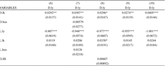
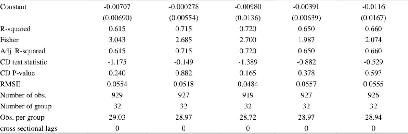
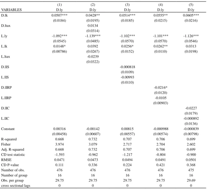
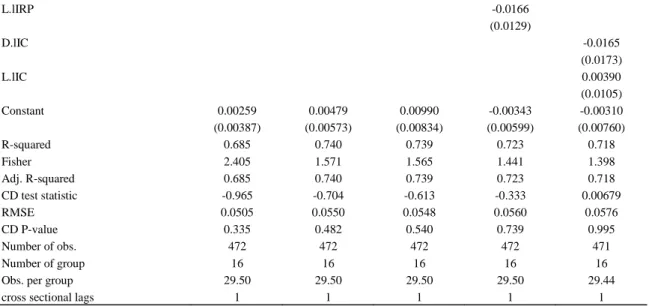
∆ ln 𝑌𝑖𝑡= 𝜋𝑖𝑐ln(𝑌𝑖𝑡−1) − ∑ 𝜋𝑖𝑗 ln(𝑋𝑖𝑡−1 j ) 𝑗 − ∑ 𝜋𝑚 𝑖𝑚ln( 𝑇𝑖𝑡−1𝑚 )+ ∑ 𝑏𝑖𝑗∆ln(𝑋𝑖𝑡 j ) 𝑗 + ∑ 𝑏𝑚 𝑖𝑚∆ln(𝑇𝑖𝑡m) + 𝜋𝑖𝑐ln(Y̅̅̅̅̅̅̅̅̅̅ + ∑ 𝜋t−1) 𝑖𝑗ln(𝑋𝑖𝑡−1 j ) ̅̅̅̅̅̅̅̅̅̅̅̅ 𝑗 + ∑ 𝜋𝑚 𝑖𝑚ln( 𝑇̅̅̅̅̅̅̅̅̅̅̅̅𝑖𝑡−1𝑚 )+ 𝑠𝑖 ∆ ln 𝑌̅̅̅̅̅̅̅𝑡+ ∑ 𝑠𝑖𝑗∆ln(𝑋𝑖𝑡 j ) ̅̅̅̅̅̅̅̅̅̅̅ 𝑗 + ∑ 𝑠𝑚 𝑖𝑚̅̅̅̅̅̅̅̅̅̅̅∆ln(𝑇𝑖𝑡m)+ 𝑠𝑖 ∆ ln 𝑌̅̅̅̅̅̅̅𝑡− + ∑ 𝑠𝑖𝑗∆ln(𝑋𝑖𝑡− j ) ̅̅̅̅̅̅̅̅̅̅̅̅̅̅ 𝑗 + ∑ 𝑠𝑚 𝑖𝑚∆ln(𝑇̅̅̅̅̅̅̅̅̅̅̅̅̅𝑖𝑡− m )+ 𝜀𝑖𝑡 (1) They suggest that the maximum number of lags "p" is equal to the cube root of temporal dimension (𝑝 = 𝑇1⁄3). We apply this procedure including trade openness and public spending. These variables into the empirical model as their average cross in order to help capture unobserved common factors, which represent the global shocks and regional benefits. Given the moderate temporal dimension of our sample, we can add a maximum delay of one year. The results are shown in Tables 5 to 8b. Tables 5 and 6 show the results for the total sample. Tables 7a and 7b show the results for RPC and Tables 8a and 8b resume the results for RRC. Results of tables 5, 7a and 8a, are obtain with addition of cross-section averages with zero lag. Results of tables 6, 7b and 8b, are obtain with addition of cross-section averages and their lagged value.
The results in Table 5 show that all long-term coefficients of tax variables remain negative and insignificant. We find a significant negative short-term effect of indirect taxes consistent with results in Table 3. In RPC (Table 7a and 7b), the long-term coefficients of tax variables are insignificant except total revenue coefficient in column 7 of table 7b. We also note that the short-term coefficient of taxes on individuals remains significantly negative. Regarding RRCs (Table 8a and 8b), it appears that the signs noted in Table 4b remain unchanged.
Table 1. Unit root test
IPS Maddala et WU Pesaran
statistique P-value statistique P-value statistique P-value
ly -14.2042 0.0000 351.8890 0.0000 -11.127 0.000 lk -1.5386 0.0620 106.6068 0.0007 -0.967 0.167 ltax -4.3892 0.0000 86.8168 0.0304 -1.991 0.023 lIS -4.5583 0.0000 131.6521 0.0000 -1.469 0.071 lIRP -4.3349 0.0000 100.6977 0.0023 -3.179 0.001 lIC -3.3953 0.0003 110.0071 0.0003 -4.352 0.000
Table 2. Unit root test
Test de Choi (2002)
Inverse 𝜒2 P-value Inverse normal P-value Inverse logit P-value Modified inverse 𝜒2 P-value
ly 411.8832 0.0000 -15.3959 0.0000 -20.0278 0.0000 30.7488 0.0000 lk 91.4255 0.0138 -1.6959 0.0449 -1.7967 0.0371 2.4241 0.0077 ltax 132.7991 0.0000 -4.7784 0.0000 -5.0071 0.0000 6.0810 0.0000 lIS 138.3071 0.0000 -4.9647 0.0000 -5.2982 0.0000 6.5679 0.0000 lIRP 129.2464 0.0000 -4.7208 0.0000 -4.8972 0.0000 5.7670 0.0000 lIC 119.9614 0.0000 -3.6316 0.0001 -3.9824 0.0001 4.9463 0.0000
Table 3. Basic model for total sample
(1) (2) (3) (4) (5)
VARIABLES D.ly D.ly D.ly D.ly D.ly
D.lk 0.0378*** 0.0344*** 0.0284** 0.0362*** 0.0385*** (0.0114) (0.0132) (0.0131) (0.0125) (0.0129) D.ltax 0.00919 (0.0196) L.ly -1.044*** -1.130*** -1.102*** -1.108*** -1.124*** (0.0454) (0.0370) (0.0453) (0.0457) (0.0424) L.lk 0.0117 0.0213 0.0105 0.0148 0.0251* (0.00989) (0.0159) (0.0116) (0.0126) (0.0136) L.ltax -0.0119 (0.0224) D.lIS -0.00222 (0.00894) L.lIS -0.00345 (0.00889) D.lIRP -0.0144 (0.0110) L.lIRP -0.0166 (0.0133) D.lIC -0.0228* (0.0127) L.lIC -0.0158 (0.0174) Constant -0.00644 -0.000109 -0.0113 -0.00441 -0.0171 (0.00517) (0.00651) (0.0117) (0.00551) (0.0169) Observations 929 927 919 927 926 R-squared 0.583 0.665 0.690 0.630 0.644 Number of groups 32 32 32 32 32 Fisher 3.677 2.804 3.101 2.408 2.554 Adj. R-squared 0.583 0.665 0.690 0.630 0.644 CD test statistic -1.207 -0.191 -1.501 -1.175 -0.968 CD P-value 0.228 0.848 0.133 0.240 0.333 RMSE 0.0572 0.0554 0.0500 0.0573 0.0569 Number of obs. 929 927 919 927 926 Number of group 32 32 32 32 32
Obs. per group 29.03 28.97 28.72 28.97 28.94
Cross sectional lags 0 0 0 0 0
Note. Standard errors in parentheses *** p<0.01, ** p<0.05, * p<0.1. Prefix “L” indicates one lag and “l” indicates variable is expressed in
Table 4a. Basic model estimate for RPC
(1) (2) (3) (4) (5)
VARIABLES D.ly D.ly D.ly D.ly D.ly
D.lk 0.0546*** 0.0449** 0.0580*** 0.0576*** 0.0645*** (0.0181) (0.0198) (0.0198) (0.0211) (0.0210) D.ltax 0.0126 (0.0333) L.ly -1.091*** -1.139*** -1.093*** -1.110*** -1.119*** (0.0569) (0.0516) (0.0599) (0.0583) (0.0572) L.lk 0.0184* 0.0464 0.0241 0.0263** 0.0371 (0.00943) (0.0287) (0.0178) (0.0109) (0.0232) L.ltax -0.0226 (0.0315) D.lIS -0.00533 (0.0113) L.lIS -0.0121 (0.0110) D.lIRP -0.0213* (0.0116) L.lIRP -0.00957 (0.00879) D.lIC -0.0184 (0.0169) L.lIC 0.00232 (0.0135) Constant 0.00401 -0.00108 0.00626 -0.00188 -0.00160 (0.00518) (0.00564) (0.00630) (0.00643) (0.00822) R-squared 0.668 0.732 0.702 0.707 0.694 Group RPC RPC RPC RPC RPC Fisher 5.466 4.031 3.478 3.571 3.343 Adj. R-squared 0.668 0.732 0.702 0.707 0.694 CD test statistic -1.613 -1.005 -1.214 -0.866 -1.095 RMSE 0.0455 0.0450 0.0475 0.0467 0.0481 CD P-value 0.107 0.315 0.225 0.387 0.273 Number of obs. 476 476 476 476 475 Number of group 16 16 16 16 16
Obs. per group 29.75 29.75 29.75 29.75 29.69
cross sectional lags 0 0 0 0 0
Note. Standard errors in parentheses *** p<0.01, ** p<0.05, * p<0.1. Prefix “L” indicates one lag and “l” indicates variable is expressed in
logarithm. “D” is the first difference operator. Table 4b. Basic model estimate for RRC
(6) (7) (8) (9) (10)
VARIABLES D.ly D.ly D.ly D.ly D.ly
D.lk 0.0292** 0.0307** 0.0296* 0.0274** 0.0405*** (0.0137) (0.0141) (0.0167) (0.0119) (0.0146) D.ltax -0.00579 (0.0277) L.ly -0.887*** -0.948*** -0.977*** -0.955*** -1.001*** (0.0619) (0.0574) (0.0607) (0.0595) (0.0672) L.lk 0.0119 0.0206 0.0330* 0.0145 0.0244 (0.0160) (0.0189) (0.0191) (0.0217) (0.0184) L.ltax 0.0126 (0.0218) D.lIS 0.00607 (0.00892)
L.lIS -0.0196 (0.0126) D.lIRP -0.0241 (0.0152) L.lIRP -0.0271 (0.0187) D.lIC 0.00298 (0.0169) L.lIC -0.0116 (0.0168) Constant -0.00368 0.00285 -0.00336 0.00212 -0.00594 (0.00814) (0.0147) (0.0117) (0.00645) (0.0217) R-squared 0.538 0.622 0.620 0.597 0.673 Group RRC RRC RRC RRC RRC Fisher 2.953 2.217 2.136 2.001 2.776 Adj. R-squared 0.538 0.622 0.620 0.597 0.673 CD test statistic 0.105 0.434 -0.558 -0.152 0.123 RMSE 0.0691 0.0689 0.0621 0.0696 0.0634 CD P-value 0.917 0.664 0.577 0.879 0.902 Number of obs. 453 451 443 451 451 Number of group 16 16 16 16 16
Obs. per group 28.31 28.19 27.69 28.19 28.19
cross sectional lags 0 0 0 0 0
Note. Standard errors in parentheses *** p<0.01, ** p<0.05, * p<0.1. Prefix “L” indicates one lag and “l” indicates variable is expressed in
logarithm. “D” is the first difference operator.
7. Conclusion
In recent years, many African countries have tried on numerous occasions to increase their GDP through taxation. The empirical evidence on this policy has not been successful despite the different data sets, methodologies and fiscal indicators used. In this context, this study sought to determine the impact of fiscal policy on growth in sub-Saharan Africa. To achieve this goal, our strategy was to empirically estimate the impact of the tax revenue on growth. The estimate was made by the DCCE estimator and taking into account the recent econometric advances. Diagnostic tests have clearly rejected the cross-data independence. Once the observed heterogeneity and unobserved heterogeneity have been properly taken into account, we have not detected any robust effect of fiscal policy on long-term growth. Our results are similar to those of Ugwunta and Ugwuanyi (2015) and N’Yilimon (2014).
Although this article focuses primarily on the long-term relationship between taxes and growth, our results draw attention to the significant negative impact of short-term indirect taxes for the total sample. This evidence, consistent with the results of Hakim Bujang and Karia (2014), suggests that a rise in indirect taxes may reduce short-term growth. Similarly, it seems that taxes on individuals are particularly harmful in poor countries with natural resources.
In terms of policy recommendations, these results imply that the use of taxation to promote growth is inappropriate, since the tax to an overall negative impact on growth in the region (although this impact is not significant). Countries should therefore continue to reform their tax systems to mitigate the distortions caused by taxation. An effective way to increase revenue and promote growth would be to work towards the emergence of a neutral tax system with respect to the behavior of economic agents in the same spirit as Lauré (1957). To achieve this goal, all countries in the region would benefit from ongoing tax reforms, by placing the logic of fiscal neutrality in the heart of the design of reform policies.
Various reforms are possible to allow the tax to generate the minimum possible distortions. A first way of reform could affect personal income tax is often perceived as inappropriate. Governments could, perhaps, move to a proportional tax, in logic of efficiency. Until the tax administration capacities are higher, this would prevent tax evasion and simplify the taxation of individuals. In this case the reduction of inequalities could be done through targeted spending.
exemptions and benefits, especially in the context of investment codes. Then, the increase in the tax base should be followed by a reduction in the different tax rates, ideally with a single nominal rate of taxation of profit which is equal to the rate actually applied. In addition, to offset the pressure on formal sector firms, the tax rate is expected to decline as a result of a stable increase in the tax base. This could boost the competitiveness of enterprises and encourage economic activity. Another area of reform concerns the depreciation system. Governments should first reduce the number of asset classes. This action would then be followed by the application of a single depreciation rate for each category. These depreciation rates should be higher than the rate normally required for the physical life of the asset to compensate for the absence of an appropriate mechanism to account for inflation that characterizes most tax regimes. Finally, decreasing depreciation should be preferred to straight-line depreciation.
Regarding indirect taxes, their potential could be improved through further reform of VAT. Many studies (see Gupta, 2007) argue that it has a greater potential to improve the performance of income in developing countries, compared to taxes on traditional products, for a number of reasons. It should therefore be to improve the policy on VAT to make some regressive. This involves the removal of VAT exemptions, to increase his plate. These exemptions (and progressive taxation) could be replaced by a spending policy targeting the poor and vulnerable households. Such initiatives would support a reduction in inequality and greater compliance with the taxation. Policymakers should also apply a single rate to avoid distorting the structure of relative prices to consumers. This practice would be more effective with a high registration threshold, so as to retain as collectors that businesses can fulfill their reporting obligations and to master their costs of collecting VAT. In addition to this, governments should work to establish an effective mechanism for repayment of structural VAT credits generated by the deduction mechanism, and end the withholding order not to affect the financial situation of companies. Finally, these recommendations can give greater results if policy makers improve their efforts to eliminate fraud, tax evasion, corruption and pursue fiscal decentralization.
This study is far from being free of any limit. One limitation is that the study focuses on the central tendency of the panel. This approach could mask the presence of nonlinearities in some countries, which are removed when you consider the average effects. Outside, as recently suggested Jaimovich and Rebelo (2012), the effects of taxation on growth could be nonlinear. Indeed, marginal increases in tax rates have little impact on growth when they are low to moderate. However, their impact on growth can be important if the rates are high. Empirical study of nonlinear effects on growth taxes would be a very relevant topic for future research.
Table 5. Robustness test total sample
(1) (2) (3) (4) (5)
VARIABLES D.ly D.ly D.ly D.ly D.ly
D.lk 0.0405*** 0.0411*** 0.0367*** 0.0368*** 0.0418*** (0.0128) (0.0153) (0.0142) (0.0132) (0.0146) D.ltax -0.00601 (0.0175) L.ly -1.054*** -1.139*** -1.124*** -1.120*** -1.146*** (0.0453) (0.0409) (0.0461) (0.0461) (0.0492) L.lk 0.0129 0.0214 0.0180 0.0172 0.0280* (0.0112) (0.0160) (0.0118) (0.0127) (0.0163) L.ltax -0.0135 (0.0221) D.lIS -0.00354 (0.00842) L.lIS -0.00681 (0.00995) D.lIRP -0.00760 (0.00988) L.lIRP -0.0149 (0.0128) D.lIC -0.0217** (0.00976) L.lIC -0.0101
Constant -0.00707 -0.000278 -0.00980 -0.00391 -0.0116 (0.00690) (0.00554) (0.0136) (0.00639) (0.0167) R-squared 0.615 0.715 0.720 0.650 0.660 Fisher 3.043 2.685 2.700 1.987 2.074 Adj. R-squared 0.615 0.715 0.720 0.650 0.660 CD test statistic -1.175 -0.149 -1.389 -0.882 -0.529 CD P-value 0.240 0.882 0.165 0.378 0.597 RMSE 0.0554 0.0518 0.0484 0.0557 0.0555 Number of obs. 929 927 919 927 926 Number of group 32 32 32 32 32
Obs. per group 29.03 28.97 28.72 28.97 28.94
cross sectional lags 0 0 0 0 0
Note. Standard errors in parentheses *** p<0.01, ** p<0.05, * p<0.1. Prefix “L” indicates one lag and “l” indicates variable is expressed in
logarithm. “D” is the first difference operator.
Table 6. Robustness test total sample
(6) (7) (8) (9) (10)
VARIABLES D.ly D.ly D.ly D.ly D.ly
D.lk 0.0463*** 0.0536*** 0.0287 0.0693*** 0.0550*** (0.0141) (0.0184) (0.0249) (0.0218) (0.0174) D.ltax -0.00725 (0.0260) L.ly -1.052*** -1.133*** -1.172*** -1.208*** -1.190*** (0.0518) (0.0578) (0.0705) (0.0597) (0.0523) L.lk 0.0241* 0.0443** 0.0179 0.0468** 0.0445** (0.0137) (0.0197) (0.0152) (0.0202) (0.0189) L.ltax -0.00532 (0.0262) D.lIS 0.00795 (0.0111) L.lIS -0.00147 (0.0172) D.lIRP 0.00428 (0.0213) L.lIRP 0.000296 (0.0244) D.lIC -0.0345** (0.0143) L.lIC -0.0367 (0.0267) Constant -0.00566 0.00366 -0.00423 0.0167 0.00383 (0.00759) (0.00984) (0.0170) (0.0153) (0.0193) R-squared 0.599 0.736 0.743 0.672 0.707 Fisher 1.523 1.356 1.373 0.997 1.175 Adj. R-squared 0.599 0.736 0.743 0.672 0.707 CD test statistic -1.399 0.0590 -0.976 0.362 -1.531 CD P-value 0.162 0.953 0.329 0.717 0.126 RMSE 0.0570 0.0530 0.0477 0.0588 0.0573 Number of obs. 905 904 896 904 904 Number of group 32 32 32 32 32
Obs. per group 28.28 28.25 28 28.25 28.25
cross sectional lags 1 1 1 1 1
Note. Standard errors in parentheses *** p<0.01, ** p<0.05, * p<0.1. Prefix “L” indicates one lag and “l” indicates variable is expressed in
Table 7a. Robustness test for RPC
(1) (2) (3) (4) (5)
VARIABLES D.ly D.ly D.ly D.ly D.ly
D.lk 0.0507*** 0.0428** 0.0514*** 0.0555** 0.0605*** (0.0184) (0.0195) (0.0185) (0.0215) (0.0216) D.ltax 0.0134 (0.0314) L.ly -1.092*** -1.139*** -1.102*** -1.101*** -1.126*** (0.0545) (0.0485) (0.0570) (0.0570) (0.0546) L.lk 0.0148* 0.0392 0.0256* 0.0262** 0.0313 (0.00786) (0.0267) (0.0152) (0.0110) (0.0198) L.ltax -0.0239 (0.0322) D.lIS -0.000818 (0.0109) L.lIS -0.00993 (0.0110) D.lIRP -0.0216* (0.0120) L.lIRP -0.0105 (0.00903) D.lIC -0.0227 (0.0179) L.lIC -0.000892 (0.0136) Constant 0.00316 -0.00142 0.00815 -0.000988 -0.000839 (0.00458) (0.00607) (0.00557) (0.00574) (0.00798) R-squared 0.668 0.732 0.707 0.706 0.699 Fisher 3.974 3.079 2.717 2.704 2.602 Adj. R-squared 0.668 0.732 0.707 0.706 0.699 CD test statistic -1.593 -0.962 -1.217 -0.804 -0.900 RMSE 0.0471 0.0473 0.0494 0.0491 0.0501 CD P-value 0.111 0.336 0.224 0.421 0.368 Number of obs. 476 476 476 476 475 Number of group 16 16 16 16 16
Obs. per group 29.75 29.75 29.75 29.75 29.69
cross sectional lags 0 0 0 0 0
Note. Standard errors in parentheses *** p<0.01, ** p<0.05, * p<0.1. Prefix “L” indicates one lag and “l” indicates variable is expressed in
logarithm. “D” is the first difference operator. Table7b. Robustness test for RPC
(6) (7) (8) (9) (10)
VARIABLES D.ly D.ly D.ly D.ly D.ly
D.lk 0.0578*** 0.0734** 0.0582** 0.0480** 0.0606* (0.0192) (0.0316) (0.0226) (0.0233) (0.0327) D.ltax 0.0149 (0.0316) L.ly -1.109*** -1.114*** -1.150*** -1.143*** -1.186*** (0.0512) (0.0662) (0.0674) (0.0665) (0.0543) L.lk 0.0146** 0.0573* 0.0180 0.0221** 0.0442 (0.00713) (0.0297) (0.0210) (0.0102) (0.0269) L.ltax -0.0401* (0.0214) D.lIS 0.00597 (0.0108) L.lIS 0.000570 (0.0113) D.lIRP -0.0219* (0.0131)
L.lIRP -0.0166 (0.0129) D.lIC -0.0165 (0.0173) L.lIC 0.00390 (0.0105) Constant 0.00259 0.00479 0.00990 -0.00343 -0.00310 (0.00387) (0.00573) (0.00834) (0.00599) (0.00760) R-squared 0.685 0.740 0.739 0.723 0.718 Fisher 2.405 1.571 1.565 1.441 1.398 Adj. R-squared 0.685 0.740 0.739 0.723 0.718 CD test statistic -0.965 -0.704 -0.613 -0.333 0.00679 RMSE 0.0505 0.0550 0.0548 0.0560 0.0576 CD P-value 0.335 0.482 0.540 0.739 0.995 Number of obs. 472 472 472 472 471 Number of group 16 16 16 16 16
Obs. per group 29.50 29.50 29.50 29.50 29.44
cross sectional lags 1 1 1 1 1
Note. Standard errors in parentheses *** p<0.01, ** p<0.05, * p<0.1. Prefix “L” indicates one lag and “l” indicates variable is expressed in logarithm. “D” is the first difference operator.
Table 8a. Robustness test for RRC
(1) (2) (3) (4) (5)
VARIABLES D.ly D.ly D.ly D.ly D.ly
D.lk 0.0352** 0.0382*** 0.0341** 0.0299** 0.0471*** (0.0145) (0.0145) (0.0166) (0.0124) (0.0156) D.ltax -0.0102 (0.0271) L.ly -0.894*** -0.956*** -0.992*** -0.959*** -0.998*** (0.0605) (0.0589) (0.0629) (0.0568) (0.0703) L.lk 0.0116 0.0206 0.0312 0.0136 0.0254 (0.0187) (0.0212) (0.0201) (0.0238) (0.0204) L.ltax 0.0166 (0.0215) D.lIS 0.00609 (0.00851) L.lIS -0.0188 (0.0141) D.lIRP -0.0195 (0.0150) L.lIRP -0.0265 (0.0183) D.lIC -0.00124 (0.0161) L.lIC -0.0141 (0.0175) Constant -0.00350 0.00676 -0.00873 0.00195 -0.00510 (0.00917) (0.0147) (0.0183) (0.00638) (0.0247) R-squared 0.554 0.649 0.637 0.604 0.708 Fisher 2.275 1.872 1.718 1.548 2.462 Adj. R-squared 0.554 0.649 0.637 0.604 0.708 CD test statistic -0.199 0.0421 -0.782 -0.214 -0.440 RMSE 0.0707 0.0700 0.0618 0.0730 0.0630 CD P-value 0.843 0.966 0.434 0.831 0.660 Number of obs. 453 451 443 451 451 Number of group 16 16 16 16 16
Obs. per group 28.31 28.19 27.69 28.19 28.19
cross sectional lags 0 0 0 0 0
Note. Standard errors in parentheses *** p<0.01, ** p<0.05, * p<0.1. Prefix “L” indicates one lag and “l” indicates variable is expressed in
Table 8b. Robustness test for RRC
(6) (7) (8) (9) (10)
VARIABLES D.ly D.ly D.ly D.ly D.ly
D.lk 0.0366*** 0.0552** 0.0525** 0.0368* 0.0487*** (0.0117) (0.0215) (0.0217) (0.0192) (0.0177) D.ltax -0.0294 (0.0397) L.ly -0.890*** -0.942*** -0.984*** -0.992*** -0.965*** (0.0696) (0.0745) (0.0755) (0.0831) (0.0859) L.lk 0.0256 0.0282 0.0535* 0.0404 0.0423 (0.0254) (0.0290) (0.0284) (0.0322) (0.0283) L.ltax 0.0357 (0.0271) D.lIS 0.0317 (0.0379) L.lIS -0.00469 (0.0297) D.lIRP -0.0244 (0.0200) L.lIRP -0.0441 (0.0286) D.lIC -0.00292 (0.0174) L.lIC -0.0131 (0.0218) Constant -0.00112 0.0123 -0.0105 0.0115* 0.00426 (0.0101) (0.0172) (0.0269) (0.00691) (0.0239) R-squared 0.631 0.757 0.659 0.747 0.763 Fisher 1.687 1.434 0.837 1.361 1.482 Adj. R-squared 0.631 0.757 0.659 0.747 0.763 CD test statistic -0.0613 0.000736 -0.385 1.666 -0.890 RMSE 0.0705 0.0683 0.0673 0.0699 0.0681 CD P-value 0.951 0.999 0.701 0.0957 0.374 Number of obs. 445 444 436 444 444 Number of group 16 16 16 16 16
Obs. per group 27.81 27.75 27.25 27.75 27.75
cross sectional lags 1 1 1 1 1
Note. Standard errors in parentheses *** p<0.01, ** p<0.05, * p<0.1. Prefix “L” indicates one lag and “l” indicates variable is expressed in
logarithm. “D” is the first difference operator. Table 9. Country of sample
Resources poor countries Resources rich countries
Benin Lesotho Botswana Ghana
Burkina Faso Madagascar Cameroon Guinea
Burundi Malawi Central African Republic Mozambique
Cabo Verde Mali Chad Namibia
Comoros Mauritius Congo, Rep. Niger
Ethiopia Senegal Côte d’Ivoire Sierra Leone
Gambia, The Swaziland Equatorial Guinea South Africa
Guinea-Bissau Togo Gabon Tanzania
Conflict of Interests
The authors have not declared any conflict of interests.
References
Acosta, O. S. L. (2012). Tax Composition and Growth: A Broad Cross-Country Perspective. IMF Working Paper (12/257). https://doi.org/10.5089/9781616355678.001
Angelopoulos, K. E. (2007). Tax-spending policies and economic growth: theoretical predictions and evidence
from the OECD. European Journal of Political Economy, 23(4), 885-902.
https://doi.org/10.1016/j.ejpoleco.2006.10.001
Arachi, G. B. (2015). Tax structure and macroeconomic performance. International Tax and Public Finance,
22(4), 635-662. https://doi.org/10.1007/s10797-015-9364-1
Arnold, J. (2008). Do Tax Structures Affect Aggregate ? Empirical Evidence from a Panel of OECD Countries.
OECD Economics Department Working Papers (643).
Baiardi, D. P. (2017). Tax Policy and Economic Growth: Does It Really Matter? CESifo Working Paper Series (Baiardi, Donatella and Profeta, Paola and Puglisi, Riccardo and Scabrosetti, Simona, Tax Policy and Economic Growth: Does It Really Matter? (February No. 6343).
Barro, R. J. I. M. (1992). Public finance in models of economic growth. The Review of Economic Studies, 59(4), 645-661. https://doi.org/10.2307/2297991
Barro, R. J., & Lee, J. W. (2012). A New Data Set of Educational Attainment in The World, 1950-2010. Journal
of Development Economics.
Bernanke, B. S., & Gurkaynak, R. S. (2001). Is Growth Exogenous? Taking Mankiw, Romer, and Weil Seriously.
NBER Macroeconomics Annual, 16, 11-57. https://doi.org/10.1086/654431
Bird, R. M. V. (2008). Tax effort in developing countries and high income countries: The impact of corruption,
voice and accountability. Economic Analysis and Policy, 38(1), 55-71.
https://doi.org/10.1016/S0313-5926(08)50006-3
Bosworth, B., & Collins, S. M. (2003). The Empirics of Growth: An Update. Brookings Papers on Economic
Activity, 113-206. https://doi.org/10.1353/eca.2004.0002
Caballero, R. J., Farhi, E., & Gourinchas, P. O. (2008, Fall). Financial Crash, Commodity Prices, and Global Imbalances. Brookeing Papers on Economic Activity, 2008(Fall), 1-55.
Calls, S., & Jolly, D. (2012, September 26). Euro zone crisis sends stock markets tumbling Wednesday in Greece
and Spain. Retrieved from http://www.sott.net
Central Intellegence Agency. (2012). World Factbook. Retrieved from
https://www.cia.gov/library/publications/the-world-factbook/geos/wz.html#top
Chamley, C. (1986). Optimal taxation of capital income in general equilibrium with infinite lives. Econometrica:
Journal of the Econometric Society, 607-622. https://doi.org/10.2307/1911310
Chigbu, E. E. (2012). An empirical study on the causality between economic growth and taxation in Nigeria.
Current research Journal of Economic Theory, 4(2), 29-38.
Choi, I. (2001). Unit root tests for panel data. Journal of International Money and Finance, 20(2), 249-272. https://doi.org/10.1016/S0261-5606(00)00048-6
Chudik, A. E. (2015). Common correlated effects estimation of heterogeneous dynamic panel data models with
weakly exogenous regressors. Journal of Econometrics, 188(2), 393-420.
https://doi.org/10.1016/j.jeconom.2015.03.007
Chudik, A. P. (2011). Weak and strong cross ‐section dependence and estimation of large panels. The
Econometrics Journal, 14(1). https://doi.org/10.1111/j.1368-423X.2010.00330.x
Cleeve, E. (2008). How effective are fiscal incentives to attract FDI to Sub-Saharan Africa? Journal of
Developing Areas, 42(1), 135-153. https://doi.org/10.1353/jda.0.0015
Cochrane, J. H. (1991). A critique of the application of unit root tests. Journal of Economic Dynamics and
Control, 15(2), 275-284. https://doi.org/10.1016/0165-1889(91)90013-Q
Confidence, J. I. (2014). Taxation as an instrument of economic growth (The Nigerian perspective). Info. Knowl.
Manage, 12(4).
De Hoyos, R. E. (2006). Testing for cross-sectional dependence in panel-data models. Stata Journal, 6(4), 482. Déborah, I. (2011). Owning Development: Taxation to fight poverty. Oxfam Research Reports.
debt and growth. International Monetary Fund (13-248).
Edame, G. E. (2014). The impact of taxation on investment and economic development in Nigeria. Academic
Journal of Interdisciplinary Studies, 3(4), 209. https://doi.org/10.5901/ajis.2014.v3n4p209
Engen, E. M. (1996). Taxation and economic growth. National Bureau of Economic Research (w5826).
FMI. (2016). Afrique subsaharienne un changement de cap s’impose. In P. E. Régionales (Ed.), É tudes
Economiques et Financières (pp. 1-10).
Galor, O., & Moav, O. (2006). Das Human-Kapital: A Theory of the Demise of the Class Structure. Review of
Economic Studies, 73, 85-117. https://doi.org/10.1111/j.1467-937X.2006.00370.x
GRanger, C. W. (1974). Spurious regressions in econometrics. Journal of Econometrics, 2(2), 111-120. https://doi.org/10.1016/0304-4076(74)90034-7
Hakim, T. A. (2016). Does goods and services tax stimulate economic growth? International evidence. Journal of
Business and Retail Management Research, 10(3).
Hall, R. E., & Jones, C. I. (1999). Why do Some Countries Produce So Much More Output Per Worker than Others? The Quarterly Journal of Economics, 114(1), 83-116. https://doi.org/10.1162/003355399555954 Hamzaoui, M. E. (2017). Impact De La Fiscalite Sur La Croissance Economique Du Maroc. European Scientific
Journal, 13(4). https://doi.org/10.19044/esj.2017.v13n4p104
Im, K. S. (2003). Testing for unit roots in heterogeneous panels. Journal of Econometrics, 115(1), 53-74. https://doi.org/10.1016/S0304-4076(03)00092-7
Jalata, D. M. (2014). Value Added Tax as a Tool for National Development in Ethiopia. Research Journal of
Finance and Accounting, 5(15).
Jorgensen, D. W. (1967). The Theory of Investment Behavior. In R. Ferber (Ed.), Determinants of Investment
Behavior (pp. 129-188). National Bureau of Economic research.
Judd, K. L. (1985). Redistributive taxation in a simple perfect foresight model. Journal of Public Economics,
28(1), 59-83. https://doi.org/10.1016/0047-2727(85)90020-9
Keho, Y. (2010). Estimating the growth-maximizing tax rate for Cote d'Ivoire: Evidence and implications.
Journal of Economics and International Finance, 2(9), 164.
Keho, Y. (2011). Tax Structure and Economic Growth in Cote dIvoire: Are Some Taxes Better Than Others?
Asian Economic and Financial Review, 1(4), 226.
Keho, Y. (2013). The structure of taxes and economic growth in Cote d‟ Ivoire: An econometric investigation.
Journal of Research in Economics and International Finance, 2(3), 39-48.
Kneller, R. B. (1999). Fiscal policy and growth: Evidence from OECD countries. Journal of Public Economics,
74(2), 171-190. https://doi.org/10.1016/S0047-2727(99)00022-5
Lauré, M. (1953). Impôts et productivité. (L. d. Paris, Ed.) Lauré, M. (1957). Traité de politique fiscale (P. u. France, Ed.)
Lee, Y. E. (2005). Tax structure and economic growth. Journal of Public Economics, 89(5), 1027-1043. https://doi.org/10.1016/j.jpubeco.2004.07.002
Lewis, W. A. (1955). The Theory of Economic Growth. London: Allen & Unwin.
Maddala, G. S. (1999). A comparative study of unit root tests with panel data and a new simple test. Oxford
Bulletin of Economics and statistics, 61(S1), 631-652. https://doi.org/10.1111/1468-0084.61.s1.13
Maiga, S. (2015). The Impact of Tax Collection in Achieving Revenue Targets: The Directorate General of Taxes of Mali Case Study. Theoretical Economics Letters, 5(3), 403. https://doi.org/10.4236/tel.2015.53046 Mankiw, N. G., Rome, D., & Weil, D. (1992). A Contribution to the Empirics of Economic Growth. The
Quarterly Journal of Economics, 107(2), 407-437. https://doi.org/10.2307/2118477
Mansour, M. (2014). Dataset for Sub-Saharan Africa: 1980-2010. Revue D‟ É conomie du DÉ Veloppement, 22(3),
99-128.
Marquetti, A., & Foley, D. K. (2012). Extended Penn World Tables v. 4.0 - EPWT 4.0, August 2011. Retrieved from https://sites.google.com/a/newschool.edu/duncan-foley-homepage/home/EPWT