Antenna Design for Ultra Wideband Radio
by
Johnna Powell
B.S., Electrical Engineering New Mexico State University, 2001SUBMITTED TO THE DEPARTMENT OF ELECTRICAL ENGINEERING IN PARTIAL FULFILLMENT OF THE REQUIREMENTS FOR THE DEGREE OF
MASTER OF SCIENCE IN ELECTRICAL ENGINEERING
AT THE
MASSACHUSETTS INSTITUTE OF TECHNOLOGY May 7, 2004
© Massachusetts Institute of Technology All Rights Reserved
MASSACHUSETTS INSTITUTE. OF TECHNOLOGY
JUL 26
2004
LIBRARIES
Signature of A uthor ... . . . .
Department of Electrical Engin ering and mputer Science May 7, 2001
C ertified by ... . . ...
Anantha P. Chandrakasan Professor of Electrical Engineering and Computer Science Thesis Supervisor
Accepted by .
>ArX~ur C. Smith Chairman, Department Committee on Graduate Students
Antenna Design for Ultra Wideband Radio
by
Johnna Powell
Submitted to the Department of Electrical Engineering
on May 7, 2004 in Partial Fulfillment of the
Requirements for the Degree of Master of Science in Electrical Engineering
ABSTRACT
The recent allocation of the 3.1-10.6 GHz spectrum by the Federal Communications Commission
(FCC) for Ultra Wideband (UWB) radio applications has presented a myriad of exciting
opportunities and challenges for design in the communications arena, including antenna design. Ultra Wideband Radio requires operating bandwidths up to greater than 100% of the center frequency. Successful transmission and reception of an Ultra Wideband pulse that occupies the entire 3.1-10.6 GHz spectrum require an antenna that has linear phase, low dispersion and VSWR 2 throughout the entire band. Linear phase and low dispersion ensure low values of group delay, which is imperative for transmitting and receiving a pulse with minimal distortion. VSWR 2 is required for proper impedance matching throughout the band, ensuring at least 90% total
power radiation. Compatibility with an integrated circuit also requires an unobtrusive,
electrically small design. The focus of this thesis is to develop an antenna for the UWB 3.1-10.6 GHz band that achieves a physically compact, planar profile, sufficient impedance bandwidth, high radiation pattern and near omnidirectional radiation pattern.
Thesis Supervisor: Anantha P. Chandrakasan Title: Professor of Electrical Engineering
ACKNOWLEDGEMENTS
First and foremost, I would like to thank my advisor, Anantha Chandrakasan, for the opportunity to work on this project, and also for his support and confidence in my work. His patience and encouragement were invaluable to me throughout the course of this research. He pushed me to perform to the best of my abilities and gave me opportunities and exposure I never would have had if I had not joined his group. For that, I am extremely grateful. I would also like to thank the entire UWB group including Raul Blazquez, Fred Lee, David Wentzloff, Brian Ginsburg, and former student Puneet Newaskar, for their questions, suggestions, help and support. Especially I would like to thank Raul and Fred for their many suggestions and much warranted help. Fred initially proposed the need for a differential antenna, which made my investigation much more interesting. Raul was always helpful, no matter when asked. His kind and caring qualities were much appreciated.
In addition, I would also like to thank Professor David Staelin for connecting me with Lincoln Laboratory in order to perform my very necessary chamber measurements. My results were enhanced greatly with the chamber results. He also provided a great amount of insight and advice.
I would also like to thank David Bruno at Lincoln Laboratory, who conducted our
radiation experiments in the anechoic chambers. Dr. Catherine Keller and Alan Fenn were also very helpful at Lincoln Laboratory, and instrumental in connecting me with the right people.
I am grateful to many helpful people at Intel, including Evan Green, who spent a great
deal of time helping me on the discrete UWB system and providing helpful advice. Alan Waltho and Jeff Schiffer provided antenna insight, and I sincerely appreciate all of the useful discussions we had.
Antenna fabrication was made much easier with the help of Sam Lefian and Nathan Ickes, who helped with generating gerber files; Michael Garcia-Webb of the Bioinstrumentation Laboratory, who helped with the fabrication of the spiral antenna with the PCB milling router; and Chip Vaughan of the Laboratory for Manufacturing and Productivity, who provided access to the Omax waterjet, which enabled a clean circular cut of the spiral antennas.
One cannot attribute success only to work-related help. I thank, from the bottom of my heart, those who have supported me throughout these two years at MIT through their true friendship and thoughtfulness. My family has been an incredible pillar of support including my wonderful parents, Barbara and Richard, and my beautiful star athlete sister Chelsea Powell, who will never let you have a dull moment. My parents each had their own special way of making my life great. I would not be who I am if it weren't for my family, and I am so proud of them. This includes all of us- Dan, thank God you taught me about wine- one of my new passions; Betty, who's taught me to dance from the time I was five- tap, jazz and Latin ballroom; Dina, you are the goddess of cosmetology and I will never trust anyone with my hair the way I trust you; Brad, a good hearted guy who's down to earth and sensitive; Rachel, a bona fide biotechnoloist; Luke, a true gym freak; Matt, a talented Magna Cum Laude artist; Melissa, our new sister-in-law who is our most welcomed new addition to the family; and Eric, who will probably own his own ski resort someday- now you're all my family, and I love you all. My best friend Lucie Fisher, whom I have known for my whole life minus 8 months or so (I crawled up to her at the university swimming pool- yes Lucie, it was me, and now we have a written account!), talked me into going to MIT so we could be closer to each other. I have enjoyed every trip to NYC I have taken to see her since I got here. Lucie will truly be a friend for life.
People at MIT have also been a great source of comfort, including Julia Cline, who has been such a great person to have around the lab. I will miss our coffee breaks, talks and walks. She has a true life perspective; she is a secure person who is grounded and friendly, thoughtful
and sincere. Julia, I will truly miss you and wish you all the best! Frank Honore has been a great "next door neighbor", as it were. I enjoyed coming into lab to find him working at all hours, from early morning until late at night, and sharing conversations about marathons and other random topics. Margaret Flaherty helped me immensely, from keeping me on track with packing slips and receipts to making sure I got all of my reimbursements as fast as possible. She surprised me the very first day I entered lab by her warmth and pleasantness, which I was not expecting after having been semi-acclimated to the Boston attitude. Every member of "ananthagroup" has added their own flare of contribution to the culture of the lab, to make it a productive and fun place. Thanks to everyone in ananthagroup.
I'd also like to thank Debb Hodges-Pabon, who does such a great job every year
convincing the new admits to come to MIT. She is a burst of energy, joy and humor. MTL would not be the same without her. Karen Gonzalez-Valentin Gettings, who was the very first person to call me and inform me of my acceptance to MIT- you've really put things into perspective for me, and I appreciate just how sweet and genuine you are.
My grad residence, Sidney Pacific, was made much more pleasant by the camaraderie of
the Sidney Pacific officers. Working with them made my living environment so much more enjoyable. Thanks again to Michael Garcia-Webb for helping me get through the first semester, which was the hardest. I appreciated the shoulder to lean on.
I'd like to thank Chip Vaughan for his much valued friendship, for training and running
the marathon with me, and for helping me in every way imaginable just by being who he is. Chip, you're amazing.
Finally NMSU. My alma mater. My best memories. Great profs, great students, great friends. Thank you so much Dr. Russ Jedlicka, for giving me a great undergraduate research project, teaching me about antennas and making me laugh. David Brumit, thanks for being a great research buddy. Dr. Steve Castillo, Dr. Javin Taylor, Dr. Satish Ranade, Dr. Prasad, Dr. Stohaj, Dr. Bill McCarthy, Rich Turietta, and everyone I may have missed- thanks for being great teachers and mentors.
CONTENTS
ABSTRACTT ... 2 ACKNOW LEDGEMENTS ... 3 CONTENTS ... 5 FIGURES...7 INTRODUCTION ... 91.1 M otivation for Ultra W ideband Antenna Design... 11
1.2 Thesis Contribution and Overview ... 12
BACKGROUND ... 14
2.1 History of UW B ... 14
2.2 Antenna Requirements and Specifications... 15
2.2.1 Fundamental Antenna Parameters... 15
2.2.1.1 Impedance Bandwidth... 16
2.2.1.2 Radiation Pattern... 19
2.2.1.3 Half Power Beam W idth (HPBW )... 22
2.2.1.4 Directivity... 24
2.2.1.5 Efficiency ... 26
2 .2 .1.6 G ain ... 2 6 2.2.1.7 Polarization... 27
2.2.2 UW B Antenna Requirements... 28
2.3 Current and Previous Research ... 30
2.3.1 Traditional Narrowband Design... 30
2.3.2 Achieving Broader Bandwidths ... 32
2.3.3 Achieving Frequency Independence ... 35
DISCRETE PROTOTYPE ... 38
3.1 UW B Discrete System Implementation ... 38
3.2 Antenna M easurements and Time Domain Results ... 40
ANTENNA DESIGNS, SIMULATIONS AND RESULTS ...
50
4.1 Equiangular Spiral Slot Patch Antenna... 50
4.2 Narrowband M onopole Antenna... 59
4.3 Diamond Dipole Antenna... 64
4.3.1 . Sharp-Edged W ire Diamond Dipole ... 64
4.3.2 Solid Sharp Edge Diamond Dipole ... 65
4.3.3 Curved W ire Diamond Dipole ... 66
4.3.4 Curved Solid Diamond Dipole... 66
4.4.1 Design ... 68
4.4.2 CDM Results ... 69
4.5 Single Ended and Differential Elliptical Monopole Antennas (SEA and DEA) .... 72
4.5.1 Designs...72
4.5.2 Results...77
4.6 Anechoic Chamber Results ... 83
4.6.1 Single Ended and Differential Elliptical Antennas ... 85
4.6.2 Spiral Equiangular Slot Patch Antenna... 88
4.6.3 Sum m ary of Antenna Results... 89
CONCLUSIONS AND GUIDELINES FOR FUTURE WORK ... 94
5.1 Conclusions ... 94
5.2 Future W ork ... 95
A PPENDIX ... 96
APPENDIX ... 98
FIGURES
Figure 1. Diagram explanation illustrating the equivalence of a pulse based waveform
compressed in time to a signal of very wide bandwidth in the frequency domain...9
Figure 2. FCC Spectral Mask for indoor unlicensed UWB transmission. [1]. ... 10
Figure 3. Transm ission Line M odel ... 16
Figure 4: Dipole Model for Simulation and simulated 3D radiation pattern. Modeled in C ST M icrow ave Studio... 20
Figure 5. Two dimensional radiation plot for half-wave dipole: Varying 0, (p = 00 (left) and Two dimensional radiation plot for half-wave dipole: Varying $, 0 = 00 (right) ... 2 1 Figure 6. CST Microwave Studio model of horn antenna and simulated 3D radiation p attern ... 2 3 Figure 7. CST MW Studio simulated radiation pattern. Varying 0, $=00 (left). Varying $ , 0 = 0 (right)... . . 23
Figure 8. Typical microstrip patch configuration and its two dimensional radiation pattern. Modeled in CST Microwave Studio. ... 31
Figure 9. Illustrations of a biconical antenna (left) and a helical antenna (right). Models from CST M icrow ave Studio ... 33
Figure 10. Illustration of a bow-tie antenna configuration. Designed in CST Microwave S tu d io . ... 3 3 Figure 11. Rectangular loop antenna model (left) [9,10,13] and diamond dipole antenna m odel (right) [12] ... 34
Figure 12. Complementary antennas illustrating Babinet's Equivalence Principle [14].35 Figure 13. Transm it Block Diagram [15]... 38
Figure 14. UWB Discrete Transmitter Implementation based on design from Intel []. .. 39
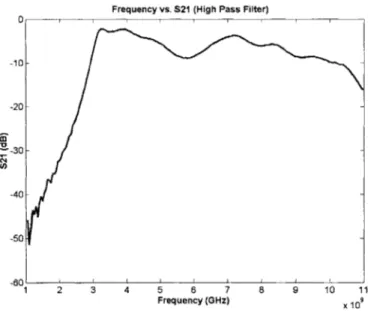
Figure 15. Output pulse from impulse generator (top) and pulse output from high pass filter...4 0 Figure 16. S21 plot of high pass filter used in discrete UWB system implementation... 41
Figure 17. Power spectrum of the transmitted pulse plotted against the FCC spectral m ask . ... 4 2 Figure 18. Top: Double Ridged Waveguide Horn Antenna (Photo courtesy ETS Lindgren, Inc.) Bottom: VSWR vs. Frequency for the Double Ridged Waveguide H orn A ntenna. ... 43
Figure 19. Return Loss vs. Frequency for Double Ridged Waveguide Horn Antenna.... 44
Figure 20. Phase vs. Frequency for Horn Antenna. ... 45
Figure 21. Group Delay vs. Frequency for Horn Antenna... 46
Figure 22. Transmitted Pulse (Dark) Superimposed on Received Pulse (Light). M easured directly at antenna terminals... 48
Figure 23. Spiral Slot Antenna Design. Remcom XFDTD simulation model...52
Figure 24. Input Impedance vs. Frequency. Results from XFDTD Simulation...53
Figure 25. S 1 (Return Loss) vs. Frequency. Results from XFDTD Simulation. ... 54
Figure 26. VSWR vs. Frequency. Results from XFDTD Simulation...54 Figure 27. Fabricated Equiangular Spiral Slot Patch Antenna. 2.5 cm radius, 0.5 cm
Figure 28. Measured VSWR vs. Frequency plot for the Equiangular Spiral Slot Patch
A n tenn a. ... 57
Figure 29. Time Domain Pulse. Received Pulse from spiral antenna superimposed on transmitted pulse. Transmit pulse is light, and receive pulse is dark... 58
Figure 30. Picture of narrowband wire antenna. ... 59
Figure 31. Measured VSWR vs. Frequency for Narrowband Wire Antenna. ... 61
Figure 32. Measured Phase vs. Frequency for Narrowband Wire Antenna...62
Figure 33. Group Delay vs. Frequency for the Narrowband Wire Antenna...62
Figure 34. Time Domain plot of wire antenna received pulse superimposed over transmitted pulse. Transmit pulse is dark, and receive pulse is light...63
Figure 35. Three configurations of a diamond dipole antenna [12] including a solid sharp-edge dipole, a wire curved-edge diamond dipole and a solid curved-edge diam ond dipole... 65
Figure 36. VSWR plots for Diamond Dipole Configurations...67
Figure 37. Circular D isc M onopole... 69
Figure 38. VSW R plot for the CDM ... 70
Figure 39. Time Domain pulse characteristics of CDM. Transmit pulse (dark) vs. R eceive pulse (light)... 7 1 Figure 40. Single Ended Elliptical Monopole Antennas...73
Figure 41. Single Ended Elliptical Monopole Antennas, measured in cm for size dem on stration ... 7 3 Figure 42. Differential Elliptical Antenna... 74
Figure 43. Measured VSWR vs. Frequency for Elliptical Monopole Antennas...77
Figure 44. Measured Phase vs. Frequency for Elliptical Antennas and Benchmark Horn A n ten n a . ... 7 9 Figure 45. Measured Group Delay for Elliptical Monopole Antennas and Benchmark H orn A ntenna. ... 79
Figure 46. Received pulse (light) over Transmit pulse (dark) for Loaded SEA...80
Figure 47. Pulse Measurement for DEA. Measured at Positive and Negative Terminals. . ... ... ... ... 81
Figure 48. Absolute value of received pulse from positive and negative terminals for the D E A ... 8 2 Figure 49. Photos of mm wavelength anechoic chambers. Courtesy David Bruno, L incoln L aboratory... 83
Figure 50. Azimuth Radiation Pattern for Loaded SEA at 4 GHz...84
Figure 51. Elevation Radiation Pattern for Loaded SEA at 4 GHz...84
Figure 52. Simulated 3-D Radiation Pattern for the Loaded SEA. Simulated in CST M icrow ave Studio. ... 87
Figure 53. Radiation pattern for Spiral Equiangular Slot Patch Antenna. Azimuth measurement shown in Blue, Elevation measurement shown in Red...89
CHAPTER
1
INTRODUCTION
Ultra Wideband Radio (UWB) is a potentially revolutionary approach to wireless communication in that it transmits and receives pulse based waveforms compressed in time rather than sinusoidal waveforms compressed in frequency. This is contrary to the traditional convention of transmitting over a very narrow bandwidth of frequency, typical of standard narrowband systems such as 802.11a, b, and Bluetooth. This enables transmission over a wide swath of frequencies such that a very low power spectral
density can be successfully received.
0
A
Frequency
A
7T~NI
A
AA.V
A
V
A\
Time
b
Figure 1. Diagram explanation illustrating the equivalence of a pulse based waveform compressed in time to a signal of very wide bandwidth in the frequency domain.
Figure 1 illustrates the equivalence of a narrowband pulse in the time domain to a signal of very wide bandwidth in the frequency domain. Also, it shows the equivalence of a
sinusoidal signal (essentially expanded in time) to a very narrow pulse in the frequency domain.
In February 2004, the FCC allocated the 3.1-10.6 GHz spectrum for unlicensed use [1]. This enabled the use and marketing of products which incorporate UWB technology. Since the allocation of the UWB frequency band, a great deal of interest has generated in industry.
The UWB spectral mask, depicted in Figure 2, was defined to allow a spectral density of -41.3 dBm/MHz throughout the UWB frequency band. Operation at such a wide bandwidth entails lower power that enables peaceful coexistence with narrowband systems. These specifications presented a myriad of opportunities and challenges to designers in a wide variety of fields including RF and circuit design, system design and
antenna design. FCC Spectral Mask -45 -50--55 -60 -65 -0 0--70 -75- -80-0 1 2 3 4 5 6 Frequency (GHz) 7 8 9 10 X I
Figure 2. FCC Spectral Mask for indoor unlicensed UWB transmission. [1].
I I I I I I I I I
.
-4"
Ultra Wideband is defined as any communication technology that occupies greater than 500 MHz of bandwidth, or greater than 25% of the operating center frequency. Most narrowband systems occupy less than 10% of the center frequency bandwidth, and are transmitted at far greater power levels. For example, if a radio system is to use the entire UWB spectrum from 3.1-10.6 GHz, and center about almost any frequency within that band, the bandwidth used would have to be greater than 100% of the center frequency in order to span the entire UWB frequency range. By contrast, the 802.1 lb radio system centers about 2.4 GHz with an operating bandwidth of 80 MHz. This communication system occupies a bandwidth of only 1% of the center frequency.
1.1 Motivation for Ultra Wideband Antenna Design
UWB has had a substantial effect on antenna design. Given that antenna research for most narrowband systems is relatively mature, coupled with the fact that the antenna has been a fundamental challenge of the UWB radio system, UWB has piqued a surge of interest in antenna design by providing new challenges and opportunities for antenna designers. The main challenge in UWB antenna design is achieving the wide impedance bandwidth while still maintaining high radiation efficiency. Spanning 7.5 GHz, almost a decade of frequency, this bandwidth goes beyond the typical definition of a wideband antenna. UWB antennas are typically required to attain a bandwidth, which reaches greater than 100% of the center frequency to ensure a sufficient impedance match is attained throughout the band such that a power loss less than 10% due to reflections occurs at the antenna terminals.
Aside from attaining a sufficient impedance bandwidth, linear phase is also required for optimal wave reception, which corresponds to near constant group delay. This minimizes pulse distortion during transmission. Also, high radiation efficiency is required especially for UWB applications. Since the transmit power is so low (below the noise floor), power loss due to dielectrics and conductor losses must be minimized. Typically, antennas sold commercially achieve efficiencies of 50-60% due to lossy dielectrics. A power loss of 50% is not acceptable for UWB since the receive end architecture already
must be exceptionally sensitive to receive a UWB signal. Extra losses could compromise the functionality of the system. The physical constraints require compatibility with portable electronic devices and integrated circuits. As such, a small and compact antenna
is required. A planar antenna is also desirable.
Given that there are several additional constraints and challenges for the design of a UWB system antenna, motivation for antenna design is clear.
1.2 Thesis Contribution and Overview
This thesis will first present a comprehensive background of the fundamental antenna parameters that should be considered in designing any antenna, narrowband or UWB. The key differences and considerations for UWB antenna design are also discussed in depth as several antennas are presented with these considerations in mind. A discrete system implementation is also discussed, in order to provide a method for which a comparison of several antennas can be made against a benchmark UWB antenna. The discrete system also provides insight into the operation of a UWB system. Time domain considerations are addressed, as well as frequency considerations including impedance matching, phase and group delay.
Several UWB antennas will be presented which were designed, simulated, tested and characterized at MIT, including a spiral equiangular slot patch antenna, a circular disc monopole, variations of a diamond dipole, and differential and single ended elliptical monopole antennas. A few of the antennas were also fabricated at MIT. Specifications such as physical profile, radiation efficiency, impedance bandwidth, phase, group delay, radiation pattern, beamwidth, gain and directivity will all be considered as various tradeoffs are discussed.
While these antenna designs and results are presented, explanation will be provided to encourage intuitive insight into how the antennas work, and why they achieve wide
bandwidth. Precious few references have contributed to an intuitive understanding of why certain antenna topologies achieve wide bandwidth.
CHAPTER
2
BACKGROUND
2.1 History of UWB
While Ultra Wideband technology may represent a revolutionary approach to wireless communication at present, it certainly is not a new concept. The first UWB radio, by definition, was the pulse-based Spark Gap radio, developed by Guglielmo Marconi in the late 1800's. This radio system was used for several decades to transmit Morse code through the airwaves. However, by 1924, Spark Gap radios were forbidden in most applications due to their strong emissions and interference to narrowband (continuous wave) radio systems, which were developed in the early 1900's. [2, 3].
By the early 1960's, increased interest in time domain electromagnetics by MIT's Lincoln Laboratory and Sperry Research Center [3] surged the development of the sampling oscilloscope by Hewlett-Packard in 1962. This enabled the analysis of the impulse response of microwave networks, and catalyzed methods for subnanosecond pulse generation. A significant research effort also was conducted by antenna designers, including Rumsey and Dyson [4, 5], who were developing logarithmic spiral antennas, and Ross, who applied impulse measurement techniques to the design of wideband, radiating antenna elements [6]. With these antenna advances, the potential for using impulse based transmission for radar and communications became clear.
Through the late 1980's, UWB technology was referred to as baseband, carrier-free or impulse technology, as the term "ultra wideband" was not used until 1989 by the U.S.
Department of Defense. Until the recent FCC allocation of the UWB spectrum for unlicensed use, all UWB applications were permissible only under a special license.
For the nearly 40 year period from 1960-1999, over 200 papers were published in accredited IEEE journals, and more than 100 patents were issued on topics related to ultra wideband technology [7]. The interest seems to be growing exponentially now, precipitated by the FCC allocation in 2002 of the UWB spectrum, with several researchers exploring RF design, circuit design, system design and antenna design, all related to UWB applications. Several business ventures have started with the hope of creating the first marketable UWB chipset, enabling revolutionary high-speed, short range data transfers and higher quality of services to the user.
2.2 Antenna Requirements and Specifications
In order to understand the challenges that UWB provides to antenna designers, a comprehensive background outlining several characterizing antenna parameters will be presented. Next, a clear description of the challenging requirements that UWB imposes with regard to these fundamental antenna parameters will be presented. Several parameters have been defined in order to characterize antennas and determine optimal applications. One very useful reference is the IEEE Standard Definitions of Terms for Antennas [8].
Several factors are considered in the simulation, design and testing of an antenna, and most of these metrics are described in 2.2.1, Fundamental Antenna Parameters. These parameters must be fully defined and explained before a thorough understanding of antenna requirements for a particular application can be achieved.
2.2.1 Fundamental Antenna Parameters
Among the most fundamental antenna parameters are impedance bandwidth, radiation pattern, directivity, efficiency and gain. Other characterizing parameters that will be discussed are half-power beamwidth, polarization and range. All of the aforementioned
antenna parameters are necessary to fully characterize an antenna and determine whether an antenna is optimized for a certain application.
2.2.1.1
Impedance Bandwidth
Impedance bandwidth indicates the bandwidth for which the antenna is sufficiently matched to its input transmission line such that 10% or less of the incident signal is lost due to reflections. Impedance bandwidth measurements include the characterization of the Voltage Standing Wave Ratio (VSWR) and return loss throughout the band of interest. VSWR and return loss are both dependent on the measurement of the reflection coefficient F. F is defined as ratio of the reflected wave Vo~ to the incident wave Vo' at a transmission line load as shown in Figure 3. Transmission Line Model, and can be calculated by equation 1. [9, 10, 11]:
Ziine
Zload
z =0
Figure 3. Transmission Line Model
Vo - = Zline - Zload Equation 1
Vo + Zline + Zload
Zine and Zioad are the transmission line impedance and the load (antenna) impedance, respectively. The voltage and current through the transmission line as a function of the distance from the load, z, are given as follows:
V(z) = Vo'e~f3Z + Vo-&p = Vo+(ejpz + Fedz)
I(z) = i/Z (Vo+ejpz - Vo-edz) = Vo+/Z0 (eipz - FeIz)
Equation 2
Equation 3
Where
P
= 2t/X.The reflection coefficient F is equivalent to the SI1 parameter of the scattering matrix. A
perfect impedance match would be indicated by F = 0. The worst impedance match is given by F = -1 or 1, corresponding to a load impedance of a short or an open.
Power reflected at the terminals of the antenna is the main concern related to impedance matching. Time-average power flow is usually measured along a transmission line to determine the net average power delivered to the load. The average incident power is given by:
Equation 4 Piave = I Vo+1
2
2Zo
The reflected power is proportional to the incident power by a multiplicative factor of I1112, as follows:
pr ave = -j12 I Vo+1 2
2Zo
The net average power delivered to the load, then, is the sum of the average incident and average reflected power:
Equation 6
Pave = - [+ 2]
2Zo
Since power delivered to the load is proportional to (1-I 2), an acceptable value of F that
enables only 10% reflected power can be calculated. This result is F= 0.3162.
When a load is not perfectly matched to the transmission line, reflections at the load cause a negative traveling wave to propagate down the transmission line. Ultimately, this creates unwanted standing waves in the transmission line. VSWR measures the ratio of the amplitudes of the maximum standing wave to the minimum standing wave, and can be calculated by the equation below:
V 1+1 IF I VSWR - ax
-Vm 1- I I
Equation 7
The typically desired value of VSWR to indicate a good impedance match is 2.0 or less. This VSWR limit is derived from the value of F calculated above.
Return loss is another measure of impedance match quality, also dependent on the value of F, or S1. Antenna return loss is calculated by the following equation:
Return Loss = -IOlogIS 1 2, or -20log(IFI). Equation 8
A good impedance match is indicated by a return loss greater than 10 dB. A summary of desired antenna impedance parameters include F<0.3162, VSWR<2, and Return Loss > 10 dB.
2.2.1.2
Radiation Pattern
One of the most common descriptors of an antenna is its radiation pattern. Radiation pattern can easily indicate an application for which an antenna will be used. For example, cell phone use would necessitate a nearly omnidirectional antenna, as the user's location is not known. Therefore, radiation power should be spread out uniformly around the user for optimal reception. However, for satellite applications, a highly directive antenna would be desired such that the majority of radiated power is directed to a specific, known location. According to the IEEE Standard Definitions of Terms for Antennas [8], an antenna radiation pattern (or antenna pattern) is defined as follows:
"a mathematical function or a graphical representation of the radiation properties of the antenna as a function of space coordinates. In most cases, the radiation pattern is determined in the far-field region and is represented as a
function
of the directional coordinates. Radiation properties include power flux density, radiation intensity, field strength, directivity phase or polarization."Three dimensional radiation patterns are measured on a spherical coordinate system indicating relative strength of radiation power in the far field sphere surrounding the antenna. On the spherical coordinate system, the x-z plane (0 measurement where P=00) usually indicates the elevation plane, while the x-y plane (q measurement where 0=90')
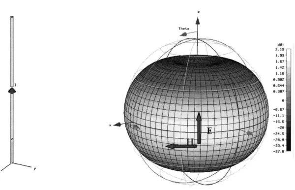
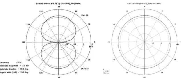
indicates the azimuth plane. Typically, the elevation plane will contain the electric-field vector (E-plane) and the direction of maximum radiation, and the azimuth plane will contain the magnetic-field vector (H-Plane) and the direction of maximum radiation. A two-dimensional radiation pattern is plotted on a polar plot with varying P or 0 for a fixed value of 0 or p, respectively. Figure 4 illustrates a half-wave dipole and its three-dimensional radiation pattern. The gain is expressed in dBi, which means that the gain is referred to an isotropic radiator. Figure 5 illustrates the two dimensional radiation patterns for varying 0 at q=00, and varying p at 0=900, respectively. It can be seen quite
clearly in Figure 4 that the maximum radiation power occurs along the 0=900 plane, or for any varying (p in the azimuth plane. The nulls in the radiation pattern occur at the ends of the dipole along the z-axis (or at 0=00 and 180*). By inspection, the two dimensional polar plots clearly show these characteristics, as well. Figure 5 shows the radiation pattern of the antenna as the value in the azimuth plane is held constant and the elevation plane (0) is varied (left), and to the right, it shows the radiation pattern of the antenna as the value in the elevation plane is held constant (in the direction of maximum radiation, 0=90') as (p varies, and no distinction in the radiation pattern is discernable.
Theta .. .. ... Ii dU i 2.19 1.93 1.67 1.42 1.16 .902 0.397. 01--6.67 -11.1- -15.6--29' -24.5 -28-9 -33.4 -37.8
Figure 4: Dipole Model for Simulation and simulated 3D radiation pattern. Modeled in CST Microwave Studio
Fartleld 'larleld p-5.34] il' Direcivity_AbsiThelas 90 120 60Phi= 90 18 0 0 - / .. -10 0 Id~il10 150 30 Frequency = 5.34
Main lobe magnitude 2.2 dB /
Main lobe direction = 90.0 deg. Phi=270 Angular width [3 dB) = 70.2 deg. 1o
90
/--/
/-Is
/.A
7./
Figure 5. Two dimensional radiation plot for half-wave dipole: Varying 0, (p = 00 (left) and Two
dimensional radiation plot for half-wave dipole: Varying , 0 = 0* (right)
While many two-dimensional radiation patterns are required for a fully complete picture of the three-dimensional radiation pattern, the two most important measurements are the E-plane and H-plane patterns. The E-plane is the plane containing the electric field vector and direction of maximum radiation, and the H-plane is the plane containing the magnetic field vector and direction of maximum radiation. While Figure 5 shows simply two "cuts" of the antenna radiation pattern, the three-dimensional pattern can clearly be inferred from these two-dimensional illustrations.
The patterns and model in Figure 4 and Figure 5 illustrate the radiation characteristics of a half-wavelength dipole, which is virtually considered an omnidirectional radiator. The only true omnidirectional radiator is that of an isotropic source, which exists only in theory. The IEEE Standard Definitions of Terms for Antennas defines an isotropic radiator as "a hypothetical lossless antenna having equal radiation in all directions." A true omnidirectional source would have no nulls in its radiation pattern, and therefore have a directivity measurement of 0 dBi. However, since no source in nature is truly isotropic, a directive antenna typically refers to an antenna that is more directive than the half-wave dipole of the figures above.
An example of a directive antenna is the Computer Simulation Technology (CST) Microwave Studio Horn antenna illustrated in Figure 6, along with its three-dimensional radiation pattern. This shows clearly the direction of maximum radiation that lies along 6
= 00, and no back radiation (or back lobes). Since this radiation pattern is simulated in an ideal environment with an infinite ground plane, no back lobe radiation has been simulated. The only lobes observable are the maximum radiation lobe and the smaller side lobes. However, in a realistic measurement conducted with a finite sized ground plane, back lobe radiation would be observed in which radiation would escape to the back of the ground plane. This simulation model suffices, however, to illustrate the radiation characteristics of a directive antenna versus the virtually omnidirectional half-wave dipole of in Figure 4 and Figure 5.
Figure 7 shows the principal E-plane and H-plane measurements of the horn antenna, clearly illustrating the characteristics indicated in the three-dimensional radiation plot. The leftmost illustration of Figure 7 holds <p constant while varying 6, while the plot on the right holds 0 constant while varying (p. A pronounced difference in the directivity of maximum radiation is clearly apparent.
2.2.1.3
Half Power Beam Width (HPBW)
Half power beamwidth (HPBW) is defined as the angular distance from the center of the main beam to the point at which the radiation power is reduced by 3 dB. This measurement is taken at two points from the center of the main beam such that this angular distance is centered about the main beam. This measurement is clearly indicated in the two dimensional plot simulations of Figure 5 and Figure 7, labeled as "Angular width (3dB)". This measurement is useful in order to describe the radiation pattern of an antenna and to indicate how directive it is.
_____________________________ -_-_-_--~.~ ~-.-~-=, ~-~ilrfl PO dBi 11.4 0.33 5.3 - 2.27 Theta -7.98 -20.7 -27.1
Figure 6. CST Microwave Studio model of horn antenna and simulated 3D radiation pattern.
Farfloid 'farleld (1=0) 111' DirectivityAbs(Thetal
90
120150 150
150 Frequency =60
Main lobe magnitude 12.9 dOi Main lobe direction = 0.0 deg.
Angular width (3 dB = 31.0 deg 120 Side lobe level = -10.8 dO
90
Farfield tforfleid (1=60] [1' DlrectviiyAb[Phl]; Theta= 0.0 deg.
90 Phi= 0 30 * N 20 Id~l! - 30 Phl=1 80 fie 120 150i . 210 Frequency =60
Main lobe magnitude = 12.9
dBa1-Main lobe direction = 355.0 deg.
240 50 30 330 300 270
Figure 7. CST MW Studio simulated radiation pattern. Varying 9, $=O* (left). Varying , 6 = 00
(right). Pul p.7 I 0 180
2.2.1.4
Directivity
According to [8], the directivity of an antenna is defined as "the ratio of the radiation intensity in a given direction from the antenna to the radiation intensity averaged over all directions. The average radiation intensity is equal to the total power radiated by the antenna divided by 47c." Directivity is more thoroughly understood theoretically when an explanation of radiation power density, radiation intensity and beam solid angle are given. References [9-11] should be referred to for more thorough explanation.
The average radiation power density is expressed as follows:
Sav = Re[EXH*] (W/m2) Equation 9
Since Say is the average power density, the total power intercepted by a closed surface can be obtained by integrating the normal component of the average power density over the entire closed surface. Then, the total radiated power is given by the following expression:
Prad = Pav = fRe(E x H*) 9 ds = #Srad ds Equation 10
S S
Radiation intensity is defined by the IEEE Standard Definitions of Terms for Antennas as "the power radiated from an antenna per unit solid angle." The radiation intensity is simply the average radiation density, Srad, scaled by the square product of the distance, r. This is also a far field approximation, and is given by:
U = r2Srad Equation 11
Where U = radiation intensity (W/unit solid angle) and Srad = radiation density (W/m2 ).
The total radiated power, Prad, can be then be found by integrating the radiation intensity over the solid angle of 47c steradians, given as:
2,ric
Prad = #JUdQ = f
JU
sin &d1#P
n 0 0
Prad = 44fUOdQ = U, (ffdi2 = 4,tUo
Equation 12
Equation 13
Where dK2 is the element of solid angle of a sphere, measured in steradians. A steradian is defined as "a unit of measure equal to the solid angle subtended at the center of a sphere by an area on the surface of the sphere that is equal to the radius squared." Integration of dQ over a spherical area as shown in the equation above yields 47t steradians. Another way to consider the steradian measurement is to consider a radian measurement: The circumference of a circle is 2ir, and there are (21rr/r) radians in a circle. The area of a sphere is 4Tr2, and there are 4Tr2/2 steradians in a sphere.
The beam solid angle is defined as the subtended area through the sphere divided by r2
dA
dQ = = - sinedOd<
r Equation 14
Given the above theoretical and mathematical explanations of radiation power density, radiation intensity and beam solid angle, a more complete understanding of antenna directivity can be achieved. Directivity is defined mathematically as:
_U 4ffU
D - U - (dimensionless) U0 P',d
Equation 15
Simply stated, antenna directivity is a measure of the ratio of the radiation intensity in a given direction to the radiation intensity that would be output from an isotropic source.
2.2.1.5
Efficiency
The antenna efficiency takes into consideration the ohmic losses of the antenna through the dielectric material and the reflective losses at the input terminals. Reflection efficiency and radiation efficiency are both taken into account to define total antenna efficiency. Reflection efficiency, or impedance mismatch efficiency, is directly related to the Si1 parameter (F). Reflection efficiency is indicated by er, and is defined
mathematically as follows:
er = (1-IFI2) = reflection efficiency Equation 16
The radiation efficiency takes into account the conduction efficiency and dielectric efficiency, and is usually determined experimentally with several measurements in an anechoic chamber. Radiation efficiency is determined by the ratio of the radiated power,
Prad to the input power at the terminals of the antenna, Pin:
P
erad = = radiation efficiency
in
Total efficiency is simply the product of the radiation efficiency. Reasonable values for total antenna efficiency 90%, although several commercial antennas achieve inexpensive, lossy dielectric materials such as FR4.
Equation 17
efficiency and the reflection are within the range of 60%
-only about 50-60% due to
2.2.1.6
Gain
The antenna gain measurement is linearly related to the directivity measurement through the antenna radiation efficiency. According to [8], the antenna absolute gain is "the ratio of the intensity, in a given direction, to the radiation intensity that would be obtained if
the power accepted by the antenna were radiated isotropically." Antenna gain is defined mathematically as follows:
G = eradD = 4t U ( (dimensionless) Equation 18
Pin
Also, if the direction of the gain measurement is not indicated, the direction of maximum gain is assumed. The gain measurement is referred to the power at the input terminals rather than the radiated power, so it tends to be a more thorough measurement, which reflects the losses in the antenna structure.
Gain measurement is typically misunderstood in terms of determining the quality of an antenna. A common misconception is that the higher the gain, the better the antenna. This is only true if the application requires a highly directive antenna. Since gain is linearly proportional to directivity, the gain measurement is a direct indication of how directive the antenna is (provided the antenna has adequate radiation efficiency).
2.2.1.7
Polarization
Antenna polarization indicates the polarization of the radiated wave of the antenna in the far-field region. The polarization of a radiated wave is the property of an electromagnetic wave describing the time varying direction and relative magnitude of the electric-field vector at a fixed location in space, and the sense in which it is traced, as observed along the direction of propagation [8]. Typically, this is measured in the direction of maximum radiation. There are three classifications of antenna polarization: linear, circular and elliptical. Circular and linear polarization are special cases of elliptical polarization. Typically, antennas will exhibit elliptical polarization to some extent. Polarization is
indicated by the electric field vector of an antenna oriented in space as a function of time. Should the vector follow a line, the wave is linearly polarized. If it follows a circle, it is circularly polarized (either with a left hand sense or right hand sense). Any other orientation is said to represent an elliptically polarized wave. Aside from the type of polarization, two main factors are taken into consideration when considering polarization of an antenna: Axial ratio and polarization mismatch loss, which can be referenced in [9-11].
2.2.2
UWB Antenna Requirements
All of the fundamental parameters described in the previous section must be considered in designing antennas for any radio application, including Ultra Wideband. However, there are additional challenges for Ultra Wideband. By definition, an Ultra Wideband antenna must be operable over the entire 3.1-10.6 GHz frequency range. Therefore, the UWB antenna must achieve almost a decade of impedance bandwidth, spanning 7.5 GHz. Another consideration that must be taken into account is group delay. Group delay is given by the derivative of the unwrapped phase of an antenna. If the phase is linear throughout the frequency range, the group delay will be constant for the frequency range. This is an important characteristic because it helps to indicate how well a UWB pulse will be transmitted and to what degree it may be distorted or dispersed. It is also a parameter that is not typically considered for narrowband antenna design because linear phase is naturally achieved for narrowband resonance. This will be discussed in greater detail in section 3.2.
Radiation pattern and radiation efficiency are also significant characteristics that must be taken into account in antenna design. A nearly omnidirectional radiation pattern is desirable in that it enables freedom in the receiver and transmitter location. This implies maximizing the half power beamwidth and minimizing directivity and gain. Conductor and dielectric losses should be minimized in order to maximize radiation efficiency. Low
loss dielectric must be used in order to maximize radiation efficiency. High radiation efficiency is imperative for an ultra wideband antenna because the transmit power spectral density is excessively low. Therefore, any excessive losses incurred by the antenna could potentially compromise the functionality of the system.
In this research, the primary application focuses on integrated circuits for portable electronic applications. Therefore, the antenna is required to be physically compact and low profile, preferably planar. Several topologies will be evaluated and presented, considering tradeoffs between each design.
For specific IC radio applications in this research, the UWB antenna requirements can be summarized in the following table:
VSWR Bandwidth 3.1 - 10.6 GHz
Radiation Efficiency High (>70%)
Phase Nearly linear; constant group delay
Radiation Pattern Omnidirectional
Directivity and Gain Low
Half Power Beamwidth Wide (> 60 0)
2.3 Current and Previous Research
While narrowband antenna research has reached a certain level of maturity, it is important to briefly describe antennas and their applications in traditional narrowband design. Following traditional narrowband design, techniques for achieving broader bandwidth are introduced in this section, and several antenna topologies are considered. Finally, Rumsey's theory of frequency independence relating to spiral antenna design is
detailed and discussed.
2.3.1 Traditional Narrowband Design
Thin dipoles and microstrip patch antennas are commonly used and are quite effective for narrowband operation. For instance, dipoles are known to virtually everyone because of their common use in cell phones, televisions and automobiles. The main reason for their ubiquitous nature is that they exhibit nearly omnidirectional radiation patterns, making transmit and receive capabilities viable for almost all locations. An example of a dipole antenna and its radiation pattern were already cited in 2.2.1.2.
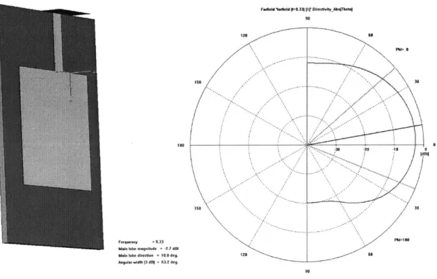
Microstrip patch antennas are generally used for aircraft, spacecraft, and even cellular communication. They can easily be designed for resonance and a desired polarization at a particular center frequency with a bandwidth of about 1% of that center frequency. In that range, return loss values of approximately 20-30 dB are achievable, with gains of approximately 2-4 dB, depending on the frequency of operation. Microstrip patch antennas are low-profile, conformable, and inexpensive to fabricate out of printed circuit board material. Figure 8 illustrates a typical microstrip patch antenna and its two-dimensional radiation pattern.
10
Reuec =.33
U. I.. . gfit de = -2.7 dli
U.i. I.b. direct n 10.0 deg.
AngtdArdth 13 dBj 53.2 deg.
FwrneWd *fild P-9.331 i Direciv1ty_AbsjThe"a
90
120 30
ISO 303
Figure 8. Typical microstrip patch configuration and its two dimensional radiation pattern. Modeled in CST Microwave Studio.
The caveat to these typical antenna designs is that they are narrowband in nature. Thin dipoles and microstrip patches exhibit reactances that converge to zero when the antenna appears as a half-wavelength transmission line to the incoming signal. Their geometry is therefore frequency dependent. However, traditional narrowband communication systems require bandwidths of several MHz for a GHz center frequency, rendering the narrowband nature of these types of antennas no substantial problem.
As mentioned previously, Ultra Wideband Radio is unique to narrowband communication systems in that it utilizes the entire 3.1-10.6 GHz band recently allocated by the FCC. UWB requires an antenna that operates sufficiently throughout the entire frequency band, such that the pulse is not distorted or dispersed during transmission and reception. Correlation schemes depend on the predictability of the pulse-shaping effects of the antenna, and as such, it is optimal to minimize pulse distortion effects.
2.3.2 Achieving Broader Bandwidths
There are many methods for broadening the bandwidth of antennas. For instance, it is well known that thickening a dipole leads to a broader bandwidth. An intuitive explanation for this follows from the fact that most of the electromagnetic energy is stored within a few wire radii of a thin dipole. Therefore, the fields are most intense around the wire radius and can be approximated by a TEM transmission line model, which corresponds to high
Q
resonance. However, as the dipole wire radius becomes thicker, the TEM transmission line model approximation breaks down and we achieve a lowerQ
resonance. Bandwidths versus length to diameter (1/d) ratios of antennas have been documented. [9,10]. For example, an antenna with a ratio l/d =5000 has an acceptable bandwidth of about 3%, which is a small fraction of the center frequency. An antenna of the same length but with a ratio l/d =260 has a bandwidth of about 30%. [9] This would correspond to a bandwidth of approximately 2.0 GHz for a center frequency of 6.5 GHz, which is still not sufficient for the entire UWB bandwidth of 7.5 GHz.There are also several known antenna topologies that are said to achieve broadband characteristics, such as the horn antenna, biconical antenna, helix antenna and bowtie antenna. An illustration of a horn antenna has been presented in Figure 6. Illustrations of a bicone and helical antenna are shown in Figure 9.
Figure 9. Illustrations of a biconical antenna (left) and a helical antenna (right). Microwave Studio.
Models from CST
While the horn, bicone and helix antenna certainly have been proven to have excellent broadband characteristics, even for the FCC allocated UWB range, they are large, non-planar and physically obtrusive, therefore ruling them out as a possibility for use with small UWB integrated electronics. However, several topologies are worth consideration. One example of a thick dipole in the form of a planar biconical antenna is the bow-tie antenna, illustrated in Figure 10.
Figure 11. Rectangular loop antenna model (left) [9,10,13] and diamond dipole antenna model (right) [12].
There are also certain polygonal configurations of the thin-wire dipole that lead to broader bandwidths, such as the triangular loop antenna proposed by Time Domain Corporation ("Diamond Dipole") [12] and the rectangular loop antenna ("Large Current Radiator") proposed by several groups as an impulse antenna [13]. Figure 11 shows embodiments of these geometrical configurations.
Intuitively, the broadband characteristics of these loop antennas is easiest to understand by inspecting their current distribution. Analyzing these dipoles as TEM transmission lines leads to the recognition that there are sharp current nulls at each edge, which creates low current standing wave ratios (SWR) even at antiresonant frequencies. The antiresonant frequencies that will see low standing wave ratios are geometrically determined. .
While these planar topologies can achieve broader bandwidths than the typical narrowband dipole or microstrip patch antenna, their frequency ranges are not broad enough to cover the 3.1-10.6 GHz band. Input reactances will cause nonlinear phase throughout the band, thereby creating distortion in the transmitted and received pulses.
2.3.3 Achieving Frequency Independence
One antenna design proposal suggests that there is a method for meeting the requirements of very wide impedance bandwidth, which uses Babinet's Equivalence Principle of duality and complementarity. [14]
Babinet's Equivalence Principle states that the product of the input impedances of two planar complementary antennas is one-quarter of the square of the characteristic
impedance of the free space: Z1Z2= 2/4.
I
/ / /r // 7 A //,~ :r A //z/j
iSi
Figure 12. Complementary antennas illustrating Babinet's Equivalence Principle [14]
Illustrated in Figure 12, antenna A is the complement of antenna B. By Babinet's
Equivalence Principle, it can be empirically and theoretically proven that ZAZB = p2/4
that ZA = ZB=r1/2 for all frequencies. This idea was first introduced by Rumsey, who proved frequency independence for an antenna whose geometry could be described solely as a function of angles in its spherical coordinate system. The following introduces Rumsey's theoretical proof for this possibility [4]:
Assuming an antenna in spherical coordinate geometry (r, 0, p) has both terminals infinitely close to the origin and each is symmetrically disposed along the 0=0, a axes, we begin by describing its surface by the curve:
r=F(0, y) Equation 19
where r represents the distance along the surface. Supposing the antenna must be scaled in size to a frequency K times lower than the original frequency, the antenna size would necessarily be scaled by K times greater. Thus, the new antenna surface would be described by
r' = KF(0, (p) Equation 20
Surfaces r and r' are identical in electrical dimensions, and congruence can be established by rotating the first antenna by an angle C so that
KF(0, 9) = F(0, p + C) Equation 21
Essentially, this means that r = r' if we move r through p in the xy-plane at angle C. It should be noted that physical congruence implies that the original antenna would behave the same at both frequencies corresponding to p and (9 + C). However, the radiation pattern would be rotated azimuthally through angle C with frequency. Because C depends on K and not 0 or p, its shape will be unaltered through its rotation. Thus, the impedance and radiation pattern will be frequency independent.
Following this proof is a derivation in order to obtain functional representation of F(0,p) by differentiating each side of the above equation with respect to C and p, and equating,
which yields
(dK/dC)F(0,p) = KaF(Op)/ ay Equation 22
1/K (dKIdC) = (1/r) ar/ 9 Equation 23
This leads to the general solution for the surface r = F(Op) of the antenna:
r = F(0,9) = ea(f(O) where a = 1/K (dK/dC) Equation 24
Thus, for any antenna to exhibit frequency independence, its surface must be described by the above equation. This geometry reflects a function of angles, independent of wavelength. Assuming the antenna has physical congruence, the infinite antenna pattern will behave the same at frequencies of any wavelength.
Babinet's Principle of Equivalence and Rumsey's theory of frequency independent geometry come together in the spiral slot antenna. This spiral curve can be derived by letting f'(0) = A8(ir/2 - 0), where A is constant and 8 is the three dimensional Dirac delta function (defined in Electromagnetic waves, [14]). Letting 0 = t/2, r = Aea(wo), where A
= roe-ao. Further derivation leads to the representation of r in wavelengths, rx = Ae
where (p = (InX)/a.
The expression of r in wavelengths shows it is evident that changing the wavelength is equivalent to varying 9, which results in nothing more than a pure rotation of the infinite
CHAPTER
3
DISCRETE PROTOTYPE
3.1 UWB Discrete System Implementation
The question to be asked is whether a degree of frequency independence, or at least "ultra" wide bandwidth might be achieved in the UWB system antenna design in order to substantially minimize or eliminate pulse distortion from a transmit to receive system. Preliminary observations of pulse-shaping effects were made on a UWB discrete system. This system was modeled after a design initially made at Intel Labs. EMCO double-ridged waveguide horn antennas with operable ranges of 1-18 GHz were used to transmit the pulses, and were used as benchmark antennas by which other antennas could be compared against. The transmitter block diagram is shown in Figure 18.
+data +out
Signal/Data --- Switch --- RF -- HPF
Generator -aa Driver -ou Switch Y
Power Impulse Splitter > Pulse Amife
Generator (ZFRC-42) Inverter
(HL9200)
This system utilizes a clock and data generator, which provides a 50 MHz clock and data synchronized with the clock. This corresponds to a pulse repetition rate (prf) of 20ns. Although a clock of 50 MHz was used for this system, a very wide range of clock frequencies could have been used for this analysis. The frequency of 50 MHz was chosen because the pulse repetition rate was long enough to resolve multipath echoes. The clock is fed to an impulse generator, which generates sub-nanosecond pulses on the order of 200ps wide. The impulse generator is split into positive and negative pulses via a power splitter and pulse inverter. The positive and negative pulses are then input to an RF switch. The RF switch is driven by a switch driver circuit, which provides a -5V drive voltage depending on the data it receives. Thus, the RF switch produces positive and negative pulses at its output depending on the data that the RF switch driver receives. The switch output is then fed to an LNA, which amplifies the signal to be transmitted via the transmit antenna. The EMCO transmit and receive antennas are operable from 1-18 GHz such that distortion is minimized. Figure 19 shows the transmit system implementation.
3.2 Antenna Measurements and Time Domain Results
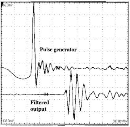
The impulse generator used in this system is an HL9200 from Hyperlabs. Powered by a 9V battery and excited by a 2V amplitude waveform, this pulse generator produces an output pulse approximately 200ps in width. Noise at the tail end of the impulse generator is present, but fortunately is substantially attenuated. After several trials with different cables, connectors, pulse repetition rates and clock voltage levels, the noise remained present, indicating that it is most likely inherent in the pulse generator. Figure 20 shows the time domain measurement of the output of the impulse generator and the filtered pulse on the TDS 8000 oscilloscope, 500ps/div and 30 mV/div.
Figure 15. Output pulse from impulse generator (top) and pulse output from high pass filter.
The top waveform of Figure 15 illustrates the output directly at the output of the impulse generator. The pulse information is very narrow, but has a wide, low frequency depression before the pulse. This depression is inherent in the impulse generator which was provided by Hyperlabs, and is caused by the step recovery diode which generates the
.... .... .. pulse generator . . . .

![Figure 14. UWB Discrete Transmitter Implementation based on design from Intel [15].](https://thumb-eu.123doks.com/thumbv2/123doknet/14016275.456969/39.918.161.760.572.950/figure-uwb-discrete-transmitter-implementation-based-design-intel.webp)