Application of linear models, random forest, and gradient boosting methods to identify key factors and predict truck dwell time for a global 3PL company
by
SireethornBenjatanont
Bachelor of Engineering, Petroleum Engineering, Chulalongkorn University, 2015 and
Dylan FranciscoTantuico
Bachelor of Science, Civil Engineering, Johns Hopkins University, 2016 SUBMITTED TO THE PROGRAM IN SUPPLY CHAIN MANAGEMENT IN PARTIAL FULFILLMENT OF THE REQUIREMENTS FOR THE DEGREE OF
MASTER OF APPLIED SCIENCE IN SUPPLY CHAIN MANAGEMENT AT THE
MASSACHUSETTS INSTITUTE OF TECHNOLOGY MAY 2020
© 2020 SireethornBenjatanont and Dylan Francisco Tantuico All rights reserved.
The authors hereby grant to MIT permission to reproduce and to distribute publicly paper and electronic copies of this capstone document in whole or in part in any medium now known or hereafter created
Signature of Author: ___________________________________________________________ SireethornBenjatanont Department of Supply Chain Management May 8, 2020 Signature of Author: ___________________________________________________________ Dylan Francisco Tantuico Department of Supply Chain Management May 8, 2020 Certified by: _________________________________________________________________ Dr. Christopher Mejia Argueta Director, MIT Food and Retail Operations Lab Capstone Advisor Certified by: _________________________________________________________________ Dr. David Correll Research Scientist, MIT Center for Transportation & Logistics Capstone Co-Advisor Accepted by: _________________________________________________________________ Dr. Yossi Sheffi Director, Center for Transportation and Logistics Elisha Gray II Professor of Engineering Systems Professor, Civil and Environmental Engineering
Application of linear models, random forest, and gradient boosting methods to identify key factors and predict truck dwell time for a global 3PL company
by
SireethornBenjatanont and
Dylan Francisco Tantuico
Submitted to the Program in Supply Chain Management on May 1, 2020 in Partial Fulfillment of the
Requirements for the Degree of Master of Applied Science in Supply Chain Management
ABSTRACT
Driver dwell time is an important challenge the U.S trucking industry faces. High, unplanned dwell times are costly to all stakeholders in the industry as they result in detention costs, declining performance and decreased driver capacity. With the increasing demand for these services, it is important to maximize the driving time of drivers in the industry by minimizing dwell time to free up capacity and provide competitive wages. This project utilizes the data of a third-party logistics company with the goal to understand the factors that influence dwell time, and to construct the model to predict dwell time of a load. In the analysis, linear models, random forest, and gradient boosting methods were explored based on regression and classification approach. Ultimately, the random forest classification model with one-hour bins is the
recommended model as it had the highest predictive performance while the one-hour bins was sufficient to meet the business need. Additionally, the analysis concludes that shipper facilities are the most significant driver of dwell time. Hence, understanding and integrating more granular observations on shipper practices within their facilities will allow a third-party logistics company to improve its driver fleet utilization and increase the predictive performance of their dwell time prediction model.
Capstone Advisor: Dr. Christopher Mejia Argueta Title: Director, MIT Food and Retail Operations Lab Capstone Co-Advisor: Dr. David Correll
ACKNOWLEDGMENTS
To our marvelous advisors, Chris and David, thank you for your tremendous support in this project. Both of you not only provide worthwhile guidance and insightful feedback in our
research results, but also give us encouragement and trust us in doing this project, which drives us to deliver the best results.
To our sponsoring company, we would like to express our gratitude to the team who supported us throughout the project. It was a pleasure to meet and work with such an amazing team that was very engaged, transparent, and helpful. We appreciate the time you took to review and discuss our work, and the valuable feedback you provided that helped shape the approach and outcome of his project.
To Toby and Pamela, thank you for your incredible help on research structure and for editing our writing. To Jen, thank you for arming us with the tools and resources available at MIT that enabled us to learn more about our topic of research.
Lastly, to the SCM Class of 2020, thank you for the friendship and support you have provided throughout this year. It was a challenging one, and we wouldn’t have made it without you. Until next time.
TABLE OF CONTENTS ABSTRACT 2 ACKNOWLEDGMENTS 3 TABLE OF CONTENTS 4 LIST OF FIGURES 6 LIST OF TABLES 7 1. Introduction 8 1.1 Overview 8 1.2 Motivation 9 1.3 Problem Statement 9 2. Literature Review 11
2.1 Overview of the Truckload Industry 11
2.2 Impact of Dwell Time in the Trucking Industry 13
2.3 Importance of Dwell Time on the Driver Experience 14
2.4 Best Practices in the Industry to Mitigate Dwell Time 16
2.5 Methodological Approaches to Quantify Dwell Time 17
2.6 Section Summary 18
3. Data and Methodology 20
3.1 Understanding the Data 20
3.1.1 Overview of Load Assignment and Delivery Process 20
3.1.2 Data Collection 23
3.2 Data Cleaning 25
3.3 Data Pre-processing 26
3.3.1 Time-related Variables 27
3.3.2 Aggregated Variables 27
3.3.3 Handling Categorical Variables 28
3.4 Model Training 29 3.4.1 Regression Approach 29 3.4.2 Classification Approach 30 3.5 Factor Analysis 34 3.5.1 Linear Models 34 3.5.2 Tree-based Models 34
3.6 Model Evaluation 35
3.6.1 Regression Metrics 35
3.6.2 Classification Metrics 36
3.6.3 Special Metric for Ordinal Outputs 37
4. Results and Analysis 39
4.1 Preliminary Exploratory Data Analysis 39
4.2 Key Factor Analysis 42
4.3 Model Performance 46
4.3.1 Regression Approach 46
4.3.2 Classification Approach 49
4.3.3 Model Performance Summary 52
5. Discussion 54
5.1 Impact of shipper facility factors on dwell time 54
5.2 Random forest classification model 55
6. Conclusion 59
References 61
LIST OF FIGURES
Figure 1: Load Assignment and Delivery Process ...20
Figure 2 Dwell time distribution in 2017-2019 ...26
Figure 3 Bar chart showing frequency of dwell time records per bin for quantile cutting ...31
Figure 4 Bar chart showing frequency of dwell time records per bin for 60-minute interval ...32
Figure 5 Bar chart showing frequency of dwell time records per bin for 6-minute interval ...32
Figure 6 Average dwell time and total number of loads delivered per hour of day per quarter ...40
Figure 7 Average number of loads fulfilled by carrier ...40
Figure 8 Total unique shippers served by carrier ...41
Figure 9 Dwell time versus total number of pallets for each load stop type ...41
Figure 10 Ridge Regression Coefficients ...43
Figure 11 Permutation Importance from Random Forest Classifier ...44
Figure 12 Permutation Importance from Random Forest Regressor ...45
Figure 13 Dwell time distribution for automated time update type ...57
LIST OF TABLES
Table 1 Minimum and maximum bounds per bin number and frequency from quantile cutting
method with 7 bins ...31
Table 2 Confusion Matrix Template ...37
Table 3 Confusion Matrix of Ridge Regression Model ...46
Table 4 Confusion Matrix of Random Forest Regression Model ...47
Table 5 Confusion Matrix of Gradient Boosting Regression Model ...48
Table 6 Confusion Matrix of Logistic Regression Model ...49
Table 7 Confusion Matrix of Random Forest Classification Model ...50
Table 8 Confusion Matrix of Gradient Boosting Classification Model ...51
1. Introduction 1.1 Overview
The U.S truckload industry is a $800 billion industry that accounts for about 80% of the nation’s entire freight cost. In 2018, 11.5 billion tons of freight were shipped by trucks around the U.S, accounting for about 70% of the total domestic tonnage shipped (ATA Reports, Trends & Statistics 2018). The industry has seen steady growth and is expected to become a $1.26 trillion-dollar industry by 2030, accounting for 25.6% growth (ATA Latest Freight Forecasts 2019). However, the industry has suffered from a shortage of drivers to fulfill the demand. The shortage was estimated to reach 60,000 drivers for 2018 and is expected to increase to 160,000 by 2028. If unmitigated, these trends will contribute to severe supply chain disruptions resulting in shipping delays, higher shipping costs, and shortages at stores (ATA Driver Shortage 2019). The sponsoring company for this project is a leading global third-party logistics provider (3PL) focused on matching drivers and shippers in the U.S Truckload Industry. The company
competes in a highly fragmented industry with 91% of the driver capacity composed by small to mid-sized entrepreneurs that operate less than 6 trucks each. Similarly, shipper demand is fragmented across multiple manufacturers, retailers, small businesses, and wholesalers with dynamic needs. This creates a highly competitive landscape for the sponsoring company and requires them to build strong relationships with their drivers and shippers to succeed.
The goal of this project is to explore how the sponsoring company can reduce driver dwell time to maximize the driving time of drivers by understanding the main factors that influence dwell time within the sponsoring company’s network, and then use statistical and machine learning techniques to predict the dwell time for each stop.
1.2 Motivation
The U.S Trucking industry imposes strict regulations on the numbers of hours driver work per day. In an industry that primarily pays per mile driven, it is important for drivers to optimize their driving time per day to maximize their earning potential. Drivers currently spend about 30% of their work week stuck loading and unloading goods at shipper facilities (OOIDA 2018).
Unpredictable dwell times result in unplanned changes to driver arrival times in shipper facilities. These unplanned schedule changes cause around 45% of drivers to lose more than 3 loads per month (OIG 2018). Moreover, these delays increase total transit times to shipper’s end
customers, not only decreasing delivery service levels, but also reducing profitability and revenue potential.
The sponsoring company aims to accurately predict dwell time at each stop to provide more accurate driver arrival times and increased schedule accuracy to its customers. Moreover, the company aims to understand the main drivers of dwell time to be able to work with its drivers and shippers to preemptively mitigate the root cause of each. Through this, the company will be able to transition from reactive dwell time firefighting to proactive shipper and driver
engagement to improve overall fleet utilization and customer satisfaction.
The motivation behind this project is to understand how the sponsoring company can predict dwell time in a shipper facility to assist in updating arrival times, improve delivery service levels, and maximize each driver’s hours of service. Reducing dwell time also improves the company’s bottom-line by reducing detention costs.
1.3 Problem Statement
This project will focus on identifying the main factors that contribute to long dwell time and predicting dwell time at each shipper’s facilities. For this project, dwell time is defined as the total time a driver spends getting loaded and unloaded at these facilities. It is a key driver of
on-time driver performance and efficient management of drivers’ fleet in the network. Hence, by spotting the main factors and achieving a more accurate prediction of dwell time, the sponsoring company will be able to provide insightful strategy to reduce unproductive time for shippers as well as increase the efficiency of drivers’ resources.
2. Literature Review
Efficient operations are becoming increasingly important for the truckload industry of the future. The growing demand, increased consumer expectations, and development of firm regulations on the industry require that firms focus on delivering greater efficiency to stay competitive (Leinbach 2007). This literature review will focus on understanding the importance of dwell time on increasing efficiency by exploring the operational and market landscape of the truckload industry, and assessing the current initiatives and approaches used to optimize it. This section starts by providing an overview of the trends and dynamics within the truckload industry, and how they relate to dwell time. Then, it expounds on the business impact dwell time has on the stakeholders involved -- the drivers, shippers, and third-party logistics companies. Lastly, it covers the best practices in industry to mitigate dwell time, and the limitations of each, and discusses current approaches to quantify dwell time through a comparison with the maritime logistics industry.
2.1 Overview of the Truckload Industry
The U.S transportation industry is a multi-billion-dollar industry dominated by trucking; therefore, the potential impact of increasing efficiency in this industry is massive.In 2018, total business logistics costs reached $1.6 trillion, 8% of GDP that year. In 2017, the trucking industry was the largest sub sector reaching $700 billion in revenues accounting for 11 billion tons of goods shipped, making up 80% of overall U.S Freight revenue. The industry is expected to grow by 2.3% year on year from 2019 through 2024 and is expected to reach a total of 15 billion tons of goods shipped by 2045 (U.S Department of Transportation 2019).
Drivers face great complexity in fulfilling shipper delivery requirements.Delivery lead times are shortening due to increased customer expectations driven by same-day and 2-day promises. With the rise of e-commerce, companies such as Amazon are requiring its competitors and
other retailers to match its increasingly aggressive delivery promise (A.T Kearney 2018). Aside from increasing the number of products being moved, the booming retail industry has increased the number of shippers on the market. Now, trucking shipper demand is made up of multiple manufacturers, wholesalers, importers, exporters and retailers each with their own locations, and pick-up and drop-off requirements. With this, knowing what, how much, and where to ship is constantly changing for drivers. Moreover, the U.S domestic trucking demand is dispersed across the entire nation.The American Trucking Research Institute suggests that trucking requirements are equally split between short and long-haul distances. Based on regional pickups and deliveries between 100-500 miles account for 37% of the total trip types in 2017, with longer distanced inter-regional, national, and shorter trips taking up about 20% each (American Trucking Research Institute 2018).
To effectively optimize its fleet, carriers in the industry need to forecast and plan the delivery demand required in the industry. As consumer spend drives the demand for domestic freight logistics, the delivery capacity of drivers in the market is required to increase. However, the demand for deliveries in the trucking industry is seasonal. Paired with the increased demand, the volatility in demand for truckload deliveries may result in imbalances in supply and demand that result in sub-optimal pricing in the full truckload and private fleet segments. During peak seasons, tight freight capacity provides leverage for drivers to raise prices and may result in increased transportation costs for shippers. With this, the United States Business logistics costs rose by 6.2% in 2017 and are expected to continue to grow over the next 5 years. Full truckload and private or dedicated fleets are expected to experience the biggest cost hikes of 4.8% and 6.8% 5-yr CAGR respectively (A.T Kearney 2018).
A survey conducted on United States truck drivers by the American Trucking Association suggests that drivers are leaving the industry in search for other jobs because they are unable to maximize their earning capacity driving on the road. Aside from the unattractive long-haul
distance and travel times, drivers face inadequate pay compared to other opportunities posed by ridesharing and similar services. Truck drivers are unable to maximize their daily earning potential due to the surprising amount of time spent waiting to be loaded and unloaded by shippers and consignees (Correll 2019). Drivers are paid per mile driven, however, they currently spend over 30% of their work week stuck loading and unloading goods at shipper facilities (OOIDA 2018).
It is becoming increasingly important to retain drivers within the industry, as the need for driver capacity increases. As the labor market in the United States continues to tighten, the industry must maximize the earning potential of drivers to provide an attractive profession and ensure their retention (Monaco 2019). Maintaining equilibrium between consumer demand and driver capacity allows for optimal pricing, an imbalance in this dynamic may result in unfavorable conditions to drivers and shippers in the form of unstable pricing and capacity that in turn affect the carrier performance and customer experience.
2.2 Impact of Dwell Time in the Trucking Industry
Currently, research has quantified the safety and economic impacts of dwell time on truck drivers. It suggests that 37% of truck driver delays are resulting from delays at shipper facilities. Moreover, this follows the release of the U.S. Department of transportation: Office of Inspector General’s (OIG) audit of customer detention impacts, which found that dwell time increased crash risks and reduced incomes for drivers and motor drivers in the for-hire sector (ATA 2019) The pressure created by this supply crunch is straining the relationship between drivers and shippers.The capacity shortage creates a driver centric market that allows drivers to prioritize routes based on profitability and preference, resulting in higher cancellations and rejections for low density and low profitable routes. Moreover, drivers have the flexibility to reject loads from shippers that take up too much time for loading/ unloading at facilities. Additionally, to increase
their potential earnings, drivers are reallocating capacity from long-term contracts to the more lucrative spot markets. As drivers act to maximize their profitability in this market, shippers are experiencing increasing pressure to fulfill customer demand while maintaining trucking costs (American Trucking Research Institute 2018).
The American Trucking Association (ATA) suggests that the capacity deficit leads to a
significant shortage in the driver workforce. Currently, carriers are addressing this shortage by increasing their efforts to recruit more drivers on the road. However, another approach to increase the industry capacity is to increase the number of hours drivers spend on the road. A study done by David Correll says that “To make up for the driver deficit, we would have to increase their driving hours to 6.7 hours per day on average — an increase of 0.2 hours or 12 minutes.”
One of the main operational challenges for drivers is to increase the time drivers can spend on the road. This project seeks to address the capacity shortage by increasing driver productivity. It aims to understand the factors that drive dwell time to ultimately predict and decrease dwell time at shipper facilities. By doing so, the project aims to help alleviate the financial pressure on drivers by allowing them to maximize driving time, and provide drivers the opportunity to optimize their daily scheduling. Increasing the productivity of drivers on the road will help stabilize the market dynamic caused by driver shortage. In short, decreasing dwell time at shipper facilities can increase industry capacity by increasing hours each driver spends on the road.
2.3 Importance of Dwell Time on the Driver Experience
Companies aim to optimize the utilization of their fleet to gain a competitive advantage in the industry (Capgemini 2016). Third-party Logistics providers have been focused on using predictive analytics to estimate the on-time delivery of their trips. A study done by Alcoba and
Ohlund in 2016, suggests that the duration a driver spends at the shipper facility (dwell time) is one of the main factors that determine whether a load is on-time or not. Moreover, the
relationship of dwell time extends to the ability to predict the estimated transit time of each trip. A study conducted by Gold Truong in 2014, examines the drivers that impact the variability of transit time estimations. The study suggests that there are three main contributing factors: variability in operations within shipper facilities, drivers driving time, and others to include external factors such as weather, accidents, traffic, etc. This study highlights the impact of dwell time on the ability of the drivers to schedule their transit times to further optimize their daily operations. A similar study conducted by Al-Habib and Favier in 2018, shows that a higher dwell time contributes to a higher load cancellation rate, costing each driver $145 dollars per load (~10% of the average total price per load), or costing the industry $4.6 billion per year. Through these examples, it is clear that predicting dwell time per load can provide drivers visibility to plan their daily schedule more flexibly, potential for savings through lower cancellations, and impact their overall experience.
Moreover, other industries have been using predictions in estimated travel times to increase customer experience. The food delivery space uses machine learning models to predict the delivery times for online customer food orders. To do so, they are able to predict the time needed for food preparation, delivery partner transit time, among other factors. The machine learning model is able to then calculate the end-to-end delivery time taking into consideration the amount of time taken at each stage of the order. This study suggests that most dwell time occurs in the restaurant, as the courier waits to receive the food to be delivered. Efforts to mitigate dwell time in restaurants by providing accurate predictions, and identifying key
operational processes in restaurants that contribute to dwell time have resulted in improving the customer experience and reducing order cancellation by 7% (Jungle Works, Predicting Arrival Time 2019).
Overall, predicting and estimating dwell time will enable drivers to budget their time more efficiently to account for the time spent at each stop. Thus, providing a better planning experience and driving more ownership of drivers on their daily operations.
2.4 Best Practices in the Industry to Mitigate Dwell Time
According to the importance of dwell time to the trucking industry, there have been multiple approaches to mitigate the dwell time and optimize supply chain efficiency. There are four possible ways to reduce the dwell time (Combined Express, Inc.n.d.)
First, shippers could provide a dock door specifically for live loads. Live load is a type of load that a driver spends time waiting at the facility as the shipper loads up the truck. As live loading is normally slower than loading a dropped trailer, separating these two types of loading will result in shorter wait times and better management of dock.
Second, shippers could require appointments for pickup and delivery time. There have been several studies dedicated to how appointment strategy could decrease dwell time. Huynh (2009) examined the impact of different scheduling policies (individual appointment system and batch appointment system) on the reduction of truck turn-time. The result demonstrates that a terminal without an appointment system could benefit from an individual appointment system by 44 percent improvement in turn time. Moreover, Zhao & Goodchild (2010) conducted the study on utilization of truck arrival time to improve yard operational efficiency and truck dwell time. The result shows that utilizing the information on truck arrival time could reduce truck transaction times within container terminals using revised difference heuristics (RDH) algorithm.
Third, drivers could leverage the trailer dropandhook method to minimize the time drivers have to spend loading and unloading at the facilities. Drop and hook is a situation when the driver
drops the trailer at the final delivery location and picks up a new trailer. The detention time is normally lower since the driver does not have to wait to load the pallets into the trailer.
Finally, shippers could set standards to filter valid and responsible drivers. This is to ensure that the selected driver is able to deliver shipping without violating regulations set by Federal Motor Carrier Safety Administration (FMCSA).
2.5 Methodological Approaches to Quantify Dwell Time
Currently, there has been limited research to quantify the amount of dwell time, particularly in the trucking industry. However, there was a similar study in maritime logistics that examined the determinant factors and developed predictive model for container dwell time.
Kourounioti et al.(2016) predicted import containers’ dwell time using artificial neural networks. They classified the relevant parameters affecting dwell time into 3 groups; container
characteristics, stakeholder’s characteristics, and terminal policies. The result of the study showed that the most important determinants of dwell time were (1) the day and month of discharge, (2) the port of origin, (3) the size and the type of container and (4) the type of cargo transferred. Moreover, it is also observed that the more input given into the model, the higher the prediction accuracy. They increased the accuracy of 14.7% in the first model with two variables, i.e., container’s size and type, to the accuracy of 65.2%, in their final model with all available variables.
Furthermore, Moini et al. (2012)outlined the framework for developing a predictive model of container dwell time and study the importance of each determinant factors affecting the
container dwell time at seaports. In this study, Naïve Bayes, decision tree, and NB-decision tree hybrid algorithm are examined with 10-fold cross validation. There are four evaluation metrics used in the study: correctly classified instances, k-statistics, root mean squared error (RMSE)
and processing time. The result shows that the best performing algorithm is the decision tree with the correctly classified instances of 0.82 for both export and import and root mean squared error of 0.19 and 0.16 days for export and import, respectively. While the Naïve Bayes perform worst with the correctly classified instances of 0.35 and 0.41 and root mean squared error of 0.29 and 0.28 days for export and import, respectively. The author suggests that future studies could expand to cover other factors such as shippers’ information.
These studies on container dwell time in the maritime logistics industry can be applied to the development of prediction algorithms for trucking dwell time. Several parameters that were examined in these studies, such as container size and type, port of origin, and type of cargo delivered, resemble those that are critical to dwell time duration in the trucking industry. 2.6 Section Summary
Customer delivery demand and the increased delivery expectation has placed increasing pressure on drivers in the U.S truckload industry. As drivers are enticed by the increasingly competitive wages and flexibility from roles in other industries, logistics companies may face difficulties in hiring and retaining drivers, thus straining the capacity to deliver goods in the industry. A mismatch between demand and capacity may lead to increasing prices and sub-optimal assignment of loads. With this, it becomes increasingly important to maximize each driver’s time on the road and provide a flexible and predictable driver experience. A few
common practices to mitigate dwell time are to utilize trailer drop-and-hook and set appointment time. To address the lack of capacity, this project focuses on understanding the factors that drive dwell time at shipper facilities to predict its duration. Moreover, while there has been limited research related to dwell time prediction in trucking industry, the framework of dwell time studies in maritime logistics study provided a valuable guideline for modelling approach as well as a benchmark for measuring predictive performance. This study will expand the scope of
existing research to cover important characteristics of the trucking industry and apply the framework to develop a predictive model.
3. Data and Methodology
This section provides an overview of the end
highlighting the key stakeholders, the responsibilities and the impact of each on dwell time to understand how the data used in the analysis is captured along the process. Then, it w discuss how the data is collected, cleaned, and processed, and provide an overview of the types of data used in the analysis of the project. Finally, it will elaborate on the analytical methods used to determine the significant factors that impact well
learning models used to predict it, and the evaluation metrics used to measure model performance.
3.1 Understanding the Data
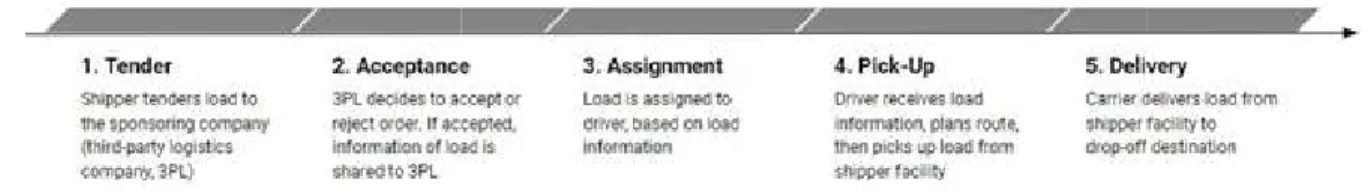
3.1.1 Overview of Load Assignment and Delivery Process Figure 1: Load Assignment
The load assignment and delivery process consist of four main phases involving multiple stakeholders. Although dwell time occurs during the loading and unloading at customer and shipper facilities, dwell time can be impacted by every
section provides an overview of the responsibility of each stakeholder at each phase, and their impact on dwell time.
Phase 1: Tender
provides an overview of the end-to-end process for load fulfillment while
highlighting the key stakeholders, the responsibilities and the impact of each on dwell time to understand how the data used in the analysis is captured along the process. Then, it w discuss how the data is collected, cleaned, and processed, and provide an overview of the types of data used in the analysis of the project. Finally, it will elaborate on the analytical methods used to determine the significant factors that impact well dwell time, the machine learning models used to predict it, and the evaluation metrics used to measure model
3.1.1 Overview of Load Assignment and Delivery Process
: Load Assignment and Delivery Process
The load assignment and delivery process consist of four main phases involving multiple stakeholders. Although dwell time occurs during the loading and unloading at customer and shipper facilities, dwell time can be impacted by every stakeholder across every phase. This section provides an overview of the responsibility of each stakeholder at each phase, and their
end process for load fulfillment while
highlighting the key stakeholders, the responsibilities and the impact of each on dwell time to understand how the data used in the analysis is captured along the process. Then, it will discuss how the data is collected, cleaned, and processed, and provide an overview of the types of data used in the analysis of the project. Finally, it will elaborate on the analytical
dwell time, the machine learning models used to predict it, and the evaluation metrics used to measure model
The load assignment and delivery process consist of four main phases involving multiple stakeholders. Although dwell time occurs during the loading and unloading at customer and
stakeholder across every phase. This section provides an overview of the responsibility of each stakeholder at each phase, and their
The shipper is the key stakeholder for this phase. Here, the shipper tenders the load to
partnering third-party logistics companies (3PL) and provides details of the load to be delivered. Tendered loads can be long-term contractual agreements that have set terms, or ad-hoc
requests in the spot market that are one-off transactions. Upon tender, shippers provide information on each load to be delivered which is shared to the 3PLs. The standard types of information included in the transactions in the industry are:
i.) Physical load attributes: Size, weight, number of pallets, type of items
ii.) Pick-up and delivery schedule: Time and location of pickup and delivery, and special operational instructions required (if any)
iii.)Shipper Information: Shipper who tendered the load
These load details shared upon tender are important to the 3PL, as they are the basis on how the 3PL will assign to its drivers. Moreover, as discussed later in the results section, the load details can be used to predict dwell time, early in the process, to allow fleet owners to further optimize their fleet. Thus, load details must be collected accurately and updated constantly. Phase 2: Acceptance
The 3PL is the key stakeholder for this phase. Upon receiving the load tender details from the shipper, the 3PL then decides whether to accept or reject the tender. If the load is accepted, the 3PL then negotiates the price to fulfill the load with the shipper. After, the 3PL assigns the load to a driver based on the load details, negotiated price, network utilization (among other factors). Moving forward, the 3PL will own all communications between the shipper and driver including managing changes in load details and scheduled times.
In load acceptance, the goal of the 3PL is to meet shipper demand and to optimize delivery fleet performance. To do so, the 3PL must effectively match drivers who can deliver loads within the cost, time, and other operational constraints provided by the shipper. The acceptance and matching process is critical in managing dwell time, as sub-optimal load assignments may result in increased dwell time within the 3PL’s system.
Phase 3: Assignment
The driver is the key stakeholder for this phase. Once the 3PL matches a driver to a load, the driver may accept or decline the request. If accepted, the driver then assumes responsibility of managing the operations required to fulfill the pickup or delivery request. Typically, each driver creates a delivery schedule that contains the time and order by which each load is picked-up/ delivered. Since drivers typically manage more than one load per day, it is in the best interest to ensure that they accept load assignments that they can meet the service level agreements for. Drivers have the option to cancel assignments for loads that are difficult and expensive to manage. Moreover, drivers often avoid loads from shippers with poor historical performance (i.e., long wait times) and predictability (i.e., changing schedules and load details). Therefore, if a driver expects a longer dwell time for a specific load, they may be incentivized to cancel the load, and therefore negatively impact the fleet’s performance and shippers experience. Phase 4: Pickup & Delivery
The shipper facilities and delivery customers are the key stakeholders for this phase. Once a load is assigned to a driver, the shippers and customers are responsible for communicating any changes within the load details or pickup/ delivery assignments to the 3PL. Providing visibility on these changes is crucial for 3PLs, as these changes must be relayed to drivers to incorporate into their daily schedule. Changes that are unaccounted for or communicated late to drivers may lead to disruptions in the operations that may contribute to increased dwell time.
Furthermore, shippers and delivery customers own the loading/ unloading operations within their facilities. The processes, equipment, manpower, and other operational resources required are determined and run solely by the shippers and delivery customers. Typically, 3PLs are not involved in determining the operations within these facilities. The length of dwell time within each facility can be directly influenced by multiple factors within a facility’s operations such as efficiency, capacity, familiarity, etc. Moreover, dwell time occurs within these facilities during this phase.
3.1.2 Data Collection
The data used in this project is collected from the sponsoring company’s internal systems that capture data on a per-load basis. Multiple data points per load are gathered throughout the entire process, starting from when the load is tendered by the shipper until when the load is delivered to the customer. The company’s internal systems use both manual processes and automated technologies to capture and record data. As requested by the sponsoring company, both methods of data collection are included in the study.
The raw data set provided includes over 19 million records of loads processed on the company’s platform from 2006 to 2019. Each load record contains about 54 unique characteristics specific to the load, and can be categorized into 3 major groups:
i.)Customer: Contains information on the shipper that requested the load and the facility where the load will be processed.
a. Shipper info:This project looks at the industry verticals and primary line of business of each shipper, as they directly impact the type of goods being transported.
b. Facility info:Each facility has a unique ID that has attached information on the location and type of operations within it. This data set covers zip, latitude and longitudinal data to
capture location, and hours of operations and other related schedules specific to the facility.
ii.)Load: Contains information on the type of load being processed, and how the load was processed.
a. Physical load attributes: These cover physical attributes of the goods to be handled before driver load acceptance, which drivers may use to evaluate whether to accept the load and to plan their operational schedule. These include the expected size and weight of the items to be delivered, when the goods need to be delivered by, and if the load was processed on the contract or spot market
b. Load processing information:This covers the attributes associated with the processing of each load, including timestamps and operational metrics, generated across each step of the process. Included here are data records on whether the load was delivered on time, how many times the load was rejected before being accepted (bounce count), whether the expected load info matched the initial request, and other operational outcomes associated with the load. The records for each load also include data on the previous and next stop such as the number of miles to the next stop, and the stop number of the current load. Most importantly, the data captures the time when a driver enters and leaves the facility. As discussed in Section 3.2 Data Cleaning, the actual dwell time per load is calculated mainly from these two data points.
iii.)Driver:Contains information on the vehicle used to fulfill the load request. These focus on capturing the type of truck and the equipment used for loading and unloading the load (drop hook vs live load). For data privacy reasons, the sponsoring company is unable to provide specific data on the driver.
All 54 data characteristics were included in the analysis(Appendix A). The goal of the project is to understand the key characteristics that drive dwell time and use them to predict the dwell time for each load.
3.2 Data Cleaning
The raw data provided by the sponsoring company includes over 19 million unique records for each load processed. The data set provided by the sponsoring company was cleaned to ensure consistent and accurate data used in the analysis. Any impurities in the data from missing entries, duplicates, or errors in encoding would result in inaccurate analyses and conclusions from the study. The data was cleaned following multiple steps documented below.
First, the dwell time of each load record was calculated by taking the total time a driver spent in the shipper facility. For unscheduled loads, the dwell time was calculated by taking the
difference between the arrival time (ArriveDateTime) and the departure time (DepartDateTime) of the driver in the facility. For scheduled loads, there are three scenarios that may result in different approaches to calculating dwell times -- the driver arrives before the scheduled arrival time, the driver arrives after the scheduled arrival time, or the driver arrives on time. For this project, if the driver arrives before the scheduled time, dwell time is defined as the difference between the scheduled arrival time and the actual departure time of the driver. This was determined by the sponsoring company to ensure highest priority on upholding delivery schedules between shippers and drivers. If the driver arrives on time or after the delivery schedule, dwell time is defined as the difference between the actual arrival time and the actual departure time of the driver, similar to the unscheduled case.
Through this process, the calculated dwell time for each load record varied widely between -780,000 hours to around 2.3 million hours. This wide range of dwell time is due to partially missing arrival time or departure time of some records. As decided with the sponsoring
company based on their domain expertise, this project’s scope focused on dwell time records between 0–6 hours, capturing the majority of the data (i.e., ~2% loss in 2017-2019 dataset). Next, due to the size of the data set and time required to process all entries, the analysis focused on the most recent 3 years, to include 2017–2019 data. Then, the data set was cleansed by removing all rows with null, blank, or duplicate entries.
In summary, the data set used in the analysis covers loads records for 3 years, from 2017 to 2019, with dwell times ranging from 0–6 hours, and complete records across all 54
characteristics included in the study. Below is the resulting distribution of dwell time.
Figure 2 Dwell time distribution in 2017-2019
Note: The dark blue line is the Kernel Density plot of the data. The light blue columns represent the continuous distribution of dwell time
3.3 Data Pre-processing
After data cleaning, data pre-processing or feature engineering is a necessary step required prior to model training. The content of data-preprocessing can be divided into three subsections. First, Section 3.3.1 will explain how to transform time-related variables. Then, Section 3.3.2 will
cover aggregated variables generated from the datasets. Lastly, Section 3.3.3 will elaborate on two methods used for handling categorical variables.
3.3.1 Time-related Variables
Time-related variables are calculated from the date and time information when a truck driver arrives at the facility.
a) Hour of Day is an integer value indicating the hour, ranging from 0–24, when a truck driver arrives at the facility.
b) Day of Week is a variable that represents the day, ranging from Monday to Sunday, when a truck driver arrives at the facility.
c) Peak Hour is a Boolean variable indicating if a truck driver arrives at the facility during the peak hour, which is between 6 AM– 4 PM.
3.3.2 Aggregated Variables
Aggregated variables are calculated using different aggregation functions, i.e., sum, unique, average, among other aggregation operations after filtering the load records by different target variables as described below.
a) Facility Traffic is the number of load records at each facility at specific hour b) Facility Complexity is the number of unique CarrierID serving specific facility c) Carrier Experience is the number of total load records served by specific driver d) Carrier Complexity is the number of unique FacilityID served by specific driver
e) Facility Historical Performancemetricsinclude average, median, min, max, and standard deviation of historical dwell time at each facility.
3.3.3 Handling Categorical Variables
There are two types of input variables in the model; numerical variables and categorical variables. While numerical variables can be inputted directly into the model, categorical variables need to be encoded before being input to the training model. Two types of encoding are selected for this capstone project to suit each model used as described below.
i.)One-Hot Encoding for Linear Models
For the nominal variables, without ordinal relationships across categories, one-hot encoding is the common preprocessing method to transform each category into another column with the value of 0 and 1 indicating whether each record falls into that specific category. This project used the one-hot encoding method prior to training the linear models, i.e., ridge regression and logistics regression. This prevents the linear model from mistakenly assigning numerical relationships among different categories when there is none.
ii.) Numerical Encoding for Tree-based Models
While one-hot encoding works well for linear models, its tendency to create a sparse input matrix especially for categorical variables with high cardinality makes it unsuitable for training tree-based models. To cope with this, another encoding technique called numerical encoding is used prior to training tree-based models, i.e., random forest and gradient boosting. Numerical encoding is a preprocessing method that transforms each category into integer values. While this type of encoding is not suitable for linear modes as it forces ordinal relationship between each category when there is none, tree-based models can handle this well as it allows more flexible and numerous splitting points.
3.4 Model Training
The modelling approaches used in this capstone project can be divided into two main
categories: regression approach and classification approach. For the regression approach, the predicted dwell time is treated as a continuous variable. While for the classification approach, the predicted dwell time is treated as a discrete variable and split into multiple bins with different binning methods. The details of each modelling technique are referenced from Géron(2019). 3.4.1 Regression Approach
Dwell time is defined as the time the truck driver spends loading and unloading the pallets at each facility and is measured in hours. Hence, the traditional modelling approach is to build a regression model to predict dwell time. There are three types of modelling techniques explored in this approach: ridge regression, random forest regression, and gradient boosting regression. i.) Ridge Regression
Ridge regression is a type of linear model, which resolves the problems of ordinary least squares in the conventional linear regression. It comprises an ordinary least squares term and an extended regularization term, called L2 penalty. The benefit of using ridge regression, as compared to conventional linear regression, is that it prevents the overfitting of the model and unusually high magnitude of coefficients. The loss function of ridge regression is based on ordinary least squares, which can be expressed as in equation (1).
𝐿(𝜃) = ∑ (𝑦( )− 𝜃𝑥( )) + 𝜃 (1)
ii.) Random Forest Regression
dependent and independent variables, the decision tree models allow multiple segmentation at each independent variable, providing more flexibility in model building. After segmenting the data, the tree model calculates and outputs the mean value of all the dependent variables within the same segment. The random forest regression works by creating multiple decision trees, each one trained on different datasets using a bagging method as well as different sets of randomly selected independent variables. The outputs from each tree are then averaged to provide the final value of prediction.
iii.) Gradient Boosting Regression
Gradient boosting regression is a type of ensemble model, which is a combination of multiple decision tree regression models. It works by sequentially adding a model that is trained on residual error from the previous prediction model.
3.4.2 Classification Approach
According to the discussion with the sponsoring company, their preferred level of prediction output is by the hour. Hence, the classification models are also explored as they could capture the preferred result in a discretized format. Prior to model training, the dwell time data was discretized into multiple bins with different binning methods. There are three types of modelling techniques explored in this approach: logistics regression, random forest classification, and gradient boosting classification.
i.) Binning Methods
Before performing the classification analysis, the dwell time data was binned by using two methods. For the first method, the bins were determined using quantile cutting, which aims to create bins with equal dwell time frequencies. The team used a trial-and-error approach to
identify the optimal number of bins that would result in an equal number of dwell time records per bin. Following this procedure resulted in 7 bins with the following divisions:
Figure 3 Bar chart showing frequency of dwell time records per bin for quantile cutting Table 1 Minimum and maximum bounds per bin number and frequency from quantile cutting method with 7 bins
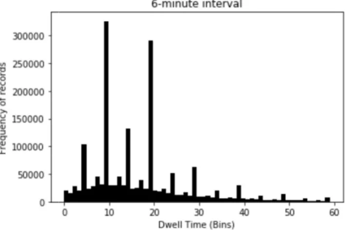
The second method, as decided with the sponsoring company, was to set bins in 6-minute and 60-minute intervals. The distribution plots are shown in Figure 4 and Figure 5. This was
operations and reporting. It is important to note that there are direct trade setting the bin size. For example, increas
data outputs, but may increase the predictive difficulty and strain model performance. On the other hand, decreasing the number of bins may increase the predictability of the data set, but may result in a loss of information due to discretization. For this analysis, the bin sizes were determined by the nature of the business of the sponsoring company, and the level of granularity required by it.
Figure 4 Bar chart showing frequenc
Figure 5 Bar chart showing frequency of dwell time records per bin for 6
operations and reporting. It is important to note that there are direct trade-offs to consider in setting the bin size. For example, increasing the number of bins may result in more granular data outputs, but may increase the predictive difficulty and strain model performance. On the other hand, decreasing the number of bins may increase the predictability of the data set, but
loss of information due to discretization. For this analysis, the bin sizes were determined by the nature of the business of the sponsoring company, and the level of
Bar chart showing frequency of dwell time records per bin for 60-minute interval
Bar chart showing frequency of dwell time records per bin for 6-minute interval offs to consider in ing the number of bins may result in more granular data outputs, but may increase the predictive difficulty and strain model performance. On the other hand, decreasing the number of bins may increase the predictability of the data set, but
loss of information due to discretization. For this analysis, the bin sizes were determined by the nature of the business of the sponsoring company, and the level of
minute interval
ii.) Logistics Regression with L2 Penalty
Logistics regression with L2 penalty is a type of linear model, which outputs the probability of occurrence of each prediction bin. The probability is calculated by taking the sigmoid function on the linear combination of independent variables as described in equation (2).
𝑝̂ = 𝜎(𝜃𝑥 + 𝜃 ) = ( ) (2)
Similar to ridge regression, it comprises a cross-entropy loss term and an extended
regularization term, called L2 penalty. Adding the L2 penalty term provides the same benefit as in ridge regression, which is to prevent the overfitting of the model and unusually high
magnitude of coefficients. The loss function of logistics regression is based on cross-entropy loss, which can be expressed as shown in equation (3).
𝐿(𝑦, 𝑝̂) = −(𝑦𝑙𝑜𝑔(𝑝̂) + (1 − 𝑦)𝑙𝑜𝑔(1 − 𝑝̂)) + 𝜃 (3)
iii.) Random Forest Classification
Similar to random forest regression, random forest classification is a type of ensemble model, which is a combination of multiple decision tree classification models. However, instead of predicting continuous variables, the model outputs are described by categories instead. iv.) Gradient Boosting Classification
Similar to gradient boosting regression, gradient boosting classification is a type of ensemble model, which is a combination of multiple decision tree regression models. However, instead of predicting continuous variables, the model outputs are described by categories instead.
3.5 Factor Analysis
After model training, the importance of each factor can be extracted using different techniques depending on the type of models (linear or tree-based). This process is called factor analysis. It is important to analyze and compare across models and understand which variables have high contribution towards dwell time, in order to formulate business suggestions that will potentially decrease the time.
3.5.1 Linear Models
The variable coefficients are the products that come from training linear models. By analyzing the magnitude and sign of coefficients related to each variable, the trend and level of impact each feature has on dwell time can be identified.
3.5.2 Tree-based Models
Feature importance is an impurity-based and common measure for factor analysis of tree-based models proposed by Breiman(2001). However, Strobl et al.(2007)pointed out that this original method is not reliable in situations when the variables vary in terms of scale of measurement and cardinalities. Since the independent variables considered in this project cover high variability of scale and cardinality, the analysis used an alternate method called permutation importance that was demonstrated by Parr et al.(2018). The permutation importance of each feature is calculated by permuting the column and measuring the difference between the baseline and the decrease in overall score. The overall score used in the regression approach is r-squared, while the overall score used in the classification approach is accuracy.
3.6 Model Evaluation
In this project, both the models under regression approach and the models under classification approach are explored. As a result, it is of utmost importance to find common ground to
compare the model across different approaches. The evaluation metrics used in this project are thoroughly selected with applied pre-processing tailored for each approach to ensure fair
judgement. The detailed calculation of regression and classification metrics are referenced from Géron(2019). While the output pre-processing techniques and special metric for ordinal outputs are proposed by the authors to match sponsoring company’s business need.
3.6.1 Regression Metrics
There are two commonly-used regression metrics chosen to evaluate the models: root mean square error (RMSE) and mean error. While the metrics can be straightforwardly applied to models in the regression approach section, for the models under classification approach, the outputs of each bin are transformed into numerical value by using the midpoint value of each bin. For example, the outputs from the 0–1 bin are converted into the value of 0.5. After that, the following two regression metrics are then applied.
i.) Root Mean Squared Error (RMSE)
Root mean squared error is a common measure of model prediction error. It tells how the predicted values differ from the actual values regardless of the sign of the differences. The formula is shown in equation (4).
ii.) Mean Error
Mean error is a common measure of model forecasting bias. Unlike RMSE, apart from prediction errors, it can also capture the event when the predictor gives unusually high or low values as compared to the actual values. The formula is shown in equation (5).
𝑀𝑒𝑎𝑛 𝑒𝑟𝑟𝑜𝑟 = ∑ (𝑦 − 𝑦 ) (5)
3.6.2 Classification Metrics
There are three commonly-used regression metrics chosen to evaluate the models: accuracy, F1 score, and confusion matrix. Contrary to section 3.6.1, the outputs from both the regression and classification models require pre-processing to convert them into common ground before comparison. This is achieved by transforming all outputs that fall into a corresponding 1-hour bin to that bin. For example, the output values of 1.05, 1.5 and 1.88 are transformed to 1–2 bin. i.) Accuracy
Accuracy is a ratio between true positives plus true negatives divided by total observations as described in equation (6).
𝐴𝑐𝑐𝑢𝑟𝑎𝑐𝑦 = (6)
ii.) F1 Score
F1 score is a metric that captures the tradeoff between precision, a ratio between true positives and total predicted positives, and recall, a ratio between true positives and total actual positives. F1 score can be calculated as described in equation (7).
𝐹1 𝑆𝑐𝑜𝑟𝑒 = × ×
iii.) Confusion Matrix
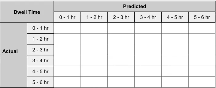
Confusion matrix is a summary table showing the total number of observations that fall into each combination of actual and predicted bins. The confusion matrix for predicted dwell time is in the following format.
Table 2 Confusion Matrix Template
Dwell Time Predicted 0 - 1 hr 1 - 2 hr 2 - 3 hr 3 - 4 hr 4 - 5 hr 5 - 6 hr Actual 0 - 1 hr 1 - 2 hr 2 - 3 hr 3 - 4 hr 4 - 5 hr 5 - 6 hr
3.6.3 Special Metric for Ordinal Outputs
While the regression metrics enable ordinal output comparison in terms of level of closeness, i.e., 2 is closer to 1 than 5, they provide the error values at excessively high detail level, which does not serve the sponsoring company’s purpose. On the contrary, while the classification metrics can be tailored to provide the evaluation at the right level of granularity (one-hour bin), it does not capture the level of closeness between ordinal outputs. In order to incorporate the benefits of both approaches, special metricfor ordinal outputs, i.e., average error by bin, is created to fulfill this purpose.
i.) Average Error by Bin
Average error by bin is obtained from the confusion matrix by calculating weighted-average value of the difference between actual and predicted data. After assigning the midpoint value to represent each bin, i.e., 1–2 bin is assigned the value of 1.5, the prediction difference for each combination of actual and predicted bin is then calculated and weighted by the number of observations in the bin.
4. Results and Analysis
This section will focus on understanding the preliminary exploratory data analysis and key factors that contribute to dwell time, and evaluating the performance of the statistical models used to predict dwell time. Section 4.1 summarizes the findings and visualizations from
exploring the datasets. Section 4.2 uses random forest models to rank the importance of each factor in the analysis, then uses a ridge regression model to explore the correlation of each factor with dwell time. Then, Section 4.3 provide the performance of allof the models. 4.1 Preliminary Exploratory Data Analysis
A descriptive analysis between each independent variable and dwell time was conducted based on the 2019 dataset to understand the correlation of each pair. The results from this exploratory analysis suggest a weak correlation between the raw variables available in the data set
provided by the sponsoring company (See Appendix A for data dictionary). To address this, the raw variables were aggregated and transformed based on various time and operational inputs (See Section 3.3.2 for results).
Figure 6 shows the heatmap tables between average dwell time and total number of loads delivered. Table on the left shows average dwell time per hour of day (y-axis), per quarter (x-axis). Table on the right shows the total number of loads delivered per hour of day (x-axis), per quarter (y-axis). The data covers loads delivered in 2019, and shows lower dwell time between the hours of 6am to 3pm, suggesting that facility hours of operations may be a significant factor impacting dwell time This is an example of an aggregated variable.
Figure 6 Average dwell time and total number of loads delivered per hour of day per quarter Figure 7 shows the average number of loads fulfilled by each carrier. The x-axis shows the average number of loads fulfilled by a carrier. The y-axis shows the average dwell time for each carrier. This figure suggests that carriers who fulfill more loads have shorter average dwell time. The data covers loads delivered in 2019. This is an example of an aggregated variable.
Shorter average dwell time for ‘active’ carriers: Carriers who have fulfilled more trips in 2019 have lower average dwell times
Figure 8 shows total unique shippers served by carrier. The x shippers served by a carrier. The y
figure suggests that carriers who serve more unique shippers tend to
times. The data covers loads delivered in 2019. This is an example of an aggregated variable.
Figure 8
Figure 9 shows dwell time versus total number of pallets for each load stop type. The x shows the total number of pallets for each unique load. The y
for each load. This figure depicts a weak correlation between dwell an example of a raw variable. The data covers loads delivered in 2019.
Figure 9Dwell time versus t
Figure 8 shows total unique shippers served by carrier. The x-axis shows the total unique shippers served by a carrier. The y-axis shows the average dwell time for each carrier. This figure suggests that carriers who serve more unique shippers tend to have higher average dwell times. The data covers loads delivered in 2019. This is an example of an aggregated variable.
8 Total unique shippers served by carrier
Figure 9 shows dwell time versus total number of pallets for each load stop type. The x
shows the total number of pallets for each unique load. The y-axis shows the average dwell time for each load. This figure depicts a weak correlation between dwell time and total pallets and is an example of a raw variable. The data covers loads delivered in 2019.
Dwell time versus total number of pallets for each load stop type axis shows the total unique axis shows the average dwell time for each carrier. This
have higher average dwell times. The data covers loads delivered in 2019. This is an example of an aggregated variable.
Figure 9 shows dwell time versus total number of pallets for each load stop type. The x-axis axis shows the average dwell time
time and total pallets and is
4.2 Key Factor Analysis
A random forest classifier and regressor were used to determine the importance of each of the factors in the model. Both models suggest that the factors capturing the historical performance of shipper facilities have the highest importance, thus suggesting that facilities play an important role in predicting the dwell time of a load. As seen on Figures 10 below, the median, average, standard deviation and maximum of historical dwell time per facility are major indicators of predicted dwell time of a load. Moreover, this analysis suggests that loads with varying load and driver factors may have the same dwell time, as determined by the facility where the loads are processed. Given that dwell time occurs within facilities, it is not alarming for these factors to be main drivers.
Aside from historical facility performance, ArriveTimeUpdateType, the method by which drivers update their arrival time at a facility, is another major driver of dwell time prediction. For this project, drivers can update their arrival time manually or automatically. Manual updates require drivers to manually input arrival timestamps in their hand-held device which may take more time, and may lead to more human error. Whereas automatic updates may rely on
radio-frequency identification (RFID) or other similar technologies attached to the driver's vehicle that captures the exact time of entry and exit of a driver in a facility. Furthermore, the results suggest that loads that are updated automatically tend to have a lower dwell time than manually updates loads.
As seen in Figure 11 and 12, several load and driver specific factors are included in the top 10 important factors that drive dwell time from the random forest regressor model. In this model, the top 2 important factors are average historical dwell time and arrival time update type. Moreover, the regressor model’s weighting is heavily skewed towards these 2 factors with Average Dwell Time (0.842) and Arrival Update Type (0.038), driving 0.88 out of 1.00 of the
importance. The other 8 factors, consisting of the driver and load factors
importance each, thus making them less relevant. The classifier model is similar to the
regressor model in that the top 2 important factors are facility driven average and median dwell time weighed 0.427 and 0.166 respectively, with arrival time update at 3rd with 0.139. Unlike the regressor model, the classifier model has mostly facility type factors in the top 10, and less variance across the weights of the top 10 factors. In aggregat
model assign equivalent weights to Average Dwell Time, Arrival Update Type, and other similar facility historical performance factors that drive over 0.90 out of 1.00 of the importance across the set of over 54 variables.
Currently, the sponsoring company does not have visibility or control over facility operations, as they are determined by each shipper. Therefore, this project will not be able to pinpoint specific operations within a facility that lead to higher dwell time.
Figure
factors, consisting of the driver and load factors contribute to importance each, thus making them less relevant. The classifier model is similar to the
regressor model in that the top 2 important factors are facility driven average and median dwell time weighed 0.427 and 0.166 respectively, with arrival time update at 3rd with 0.139. Unlike the regressor model, the classifier model has mostly facility type factors in the top 10, and less variance across the weights of the top 10 factors. In aggregate, the classifier and regressor model assign equivalent weights to Average Dwell Time, Arrival Update Type, and other similar facility historical performance factors that drive over 0.90 out of 1.00 of the importance across
rrently, the sponsoring company does not have visibility or control over facility operations, as they are determined by each shipper. Therefore, this project will not be able to pinpoint specific operations within a facility that lead to higher dwell time.
Figure 10 Ridge Regression Coefficients
contribute to ~0.01 importance each, thus making them less relevant. The classifier model is similar to the
regressor model in that the top 2 important factors are facility driven average and median dwell time weighed 0.427 and 0.166 respectively, with arrival time update at 3rd with 0.139. Unlike the regressor model, the classifier model has mostly facility type factors in the top 10, and less
e, the classifier and regressor model assign equivalent weights to Average Dwell Time, Arrival Update Type, and other similar facility historical performance factors that drive over 0.90 out of 1.00 of the importance across
rrently, the sponsoring company does not have visibility or control over facility operations, as they are determined by each shipper. Therefore, this project will not be able to pinpoint specific
Notes:-None factor corresponds to the Schedule type ‘None’ that is assigned to loads with an unknown schedule type (i.e
-Unknown factors correspond an unknown type of work (i.e Driver Assisted/ Checked).
- Clusters factors (136, 14, 99, 38, 48) correspond to anonymized geographic regions within the United States created by the sponsoring company
Figure 11 Permutation
None factor corresponds to the Schedule type ‘None’ that is assigned to loads with an unknown schedule type (i.e., By Appointment, By Notice, Open Time)
Unknown factors correspond to the Work Type ‘Unknown’ that is assigned to loads with an unknown type of work (i.e., No Touch, Driver Loaded, Driver Counted, Lumper, Driver Assisted/ Checked).
Clusters factors (136, 14, 99, 38, 48) correspond to anonymized geographic regions n the United States created by the sponsoring company
Permutation Importance from Random Forest Classifier
None factor corresponds to the Schedule type ‘None’ that is assigned to loads with an
to the Work Type ‘Unknown’ that is assigned to loads with No Touch, Driver Loaded, Driver Counted, Lumper,
Clusters factors (136, 14, 99, 38, 48) correspond to anonymized geographic regions
4.3 Model Performance
In this section, the evaluation metrics, i.e., regression metrics, classification metrics, and special metrics for ordinal outputs, of each model will be examined. Section 4.3.1 will show the model performance from the regression approach. Next, Section 4.3.2 will display the model results from the classification approach. Lastly, Section 4.3.3 will summarize and compare the performance of all of the models.
4.3.1 Regression Approach i.) Ridge Regression
After hyperparameters tuning, the regularization parameter of 0.01 was selected for final model training. The final ridge regression model has RMSE of 1.040, mean error of 0.0005, out-of-sample R2 of 0.165, accuracy of 0.370, F1 score of 0.309, and average error by bin of 0.807. The confusion matrix is displayed in Table 3.
Table 3 Confusion Matrix of Ridge Regression Model
Dwell Time Predicted 0 - 1 hr 1 - 2 hr 2 - 3 hr 3 - 4 hr 4 - 5 hr 5 - 6 hr Actual 0 - 1 hr 21,274 141,161 29,648 337 4 0 1 - 2 hr 2,902 144,632 52,208 907 11 0 2 - 3 hr 350 43,428 28,632 731 28 0 3 - 4 hr 92 15,995 17,216 741 33 0 4 - 5 hr 33 6,613 10,093 738 43 2 5 - 6 hr 16 3,161 6,031 524 64 4
ii.) Random Forest Regression
After hyperparameters tuning, the maximum depth of 10, minimum sample leaf of 3, number of trees of 300 were selected for final model training. The final random forest regression model has RMSE of 1.032, mean error of 0.0006, out-of-sample R2 of 0.179, accuracy of 0.372, F1 score of 0.307, and average error by bin of 0.800. The confusion matrix is displayed in Table 4. Table 4 Confusion Matrix of Random Forest Regression Model
Dwell Time Predicted 0 - 1 hr 1 - 2 hr 2 - 3 hr 3 - 4 hr 4 - 5 hr 5 - 6 hr Actual 0 - 1 hr 19,817 144,745 27,495 363 4 0 1 - 2 hr 2,201 147,968 49,507 964 20 0 2 - 3 hr 227 44,239 27,762 906 35 0 3 - 4 hr 56 16,233 16,830 911 46 1 4 - 5 hr 21 6,662 9,875 909 53 2 5 - 6 hr 14 3,172 5,901 635 77 1
iii.) Gradient Boosting Regression
After hyperparameters tuning, the maximum depth of 5, number of trees of 30, and learning rate of 1 were selected for final model training. The final gradient boosting regression model has RMSE of 1.031, mean error of 0.0004, out-of-sample R2 of 0.180, accuracy of 0.380, F1 score of 0.327, and average error by bin of 0.794. The confusion matrix is displayed in Table 5. Table 5 Confusion Matrix of Gradient Boosting Regression Model
Dwell Time Predicted 0 - 1 hr 1 - 2 hr 2 - 3 hr 3 - 4 hr 4 - 5 hr 5 - 6 hr Actual 0 - 1 hr 26,182 137,655 27,866 688 25 8 1 - 2 hr 3,699 144,488 50,830 1,574 64 5 2 - 3 hr 445 42,862 28,372 1,419 63 8 3 - 4 hr 126 15,643 16,793 1,438 66 11 4 - 5 hr 55 6,499 9,566 1,295 97 10 5 - 6 hr 29 2,993 5,751 900 103 24