Attribution of spring snow water equivalent (SWE) changes over the northern hemisphere to anthropogenic effects

Publisher’s version / Version de l'éditeur:

Climate Dynamics, 48, 11-12, pp. 3645-3658, 2017-07-30

READ THESE TERMS AND CONDITIONS CAREFULLY BEFORE USING THIS WEBSITE.

https://nrc-publications.canada.ca/eng/copyright

Vous avez des questions? Nous pouvons vous aider. Pour communiquer directement avec un auteur, consultez la première page de la revue dans laquelle son article a été publié afin de trouver ses coordonnées. Si vous n’arrivez pas à les repérer, communiquez avec nous à PublicationsArchive-ArchivesPublications@nrc-cnrc.gc.ca.

Questions? Contact the NRC Publications Archive team at

PublicationsArchive-ArchivesPublications@nrc-cnrc.gc.ca. If you wish to email the authors directly, please see the first page of the publication for their contact information.

NRC Publications Archive

Archives des publications du CNRC

This publication could be one of several versions: author’s original, accepted manuscript or the publisher’s version. / La version de cette publication peut être l’une des suivantes : la version prépublication de l’auteur, la version acceptée du manuscrit ou la version de l’éditeur.

For the publisher’s version, please access the DOI link below./ Pour consulter la version de l’éditeur, utilisez le lien DOI ci-dessous.

https://doi.org/10.1007/s00382-016-3291-4

Access and use of this website and the material on it are subject to the Terms and Conditions set forth at

Attribution of spring snow water equivalent (SWE) changes over the

northern hemisphere to anthropogenic effects

Jeong, Dae Il; Sushama, Laxmi; Naveed Khaliq, M.

https://publications-cnrc.canada.ca/fra/droits

L’accès à ce site Web et l’utilisation de son contenu sont assujettis aux conditions présentées dans le site LISEZ CES CONDITIONS ATTENTIVEMENT AVANT D’UTILISER CE SITE WEB.

NRC Publications Record / Notice d'Archives des publications de CNRC:

DOI 10.1007/s00382-016-3291-4

Attribution of spring snow water equivalent (SWE) changes

over the northern hemisphere to anthropogenic effects

Dae Il Jeong1 · Laxmi Sushama1 · M. Naveed Khaliq1,2

Received: 27 October 2015 / Accepted: 19 July 2016 / Published online: 30 July 2016 © The Author(s) 2016. This article is published with open access at Springerlink.com

smaller regions or with single-model signals, indicating the large uncertainty in regional SWE changes, possibly due to stronger influence of natural climate variability.

Keywords Climate change · Detection–attribution ·

Human effects · Northern Hemisphere · Snow water equivalent

1 Introduction

Snow, with its large areal extent next to sea ice among cry-osphere components, is important for regional and global land–atmosphere processes and water balance. Snow cover extent (SCE) modifies the surface albedo, thermal conduc-tivity, heat capacity, and aerodynamic roughness (Gong et al. 2004; Hancock et al. 2013) and thus also influences the atmospheric circulation. The Northern Hemisphere has about 98 % of the global snow cover (Armstrong and Brodzik 2001), which has a strong seasonal cycle and ranges (on average for 1966–2004) from 44.2 million km2 in January to 1.9 million km2 in August (Lemke et al.

2007). Snow water equivalent (SWE), a more comprehen-sive parameter than SCE that takes into account snow depth and density, has a direct influence on the hydrologic cycle and water supply in snowmelt-dominated regions (Barnett et al. 2005; Egli et al. 2009; Takala et al. 2011; Gan et al.

2013).

Observations of SCE are available from ground mete-orological stations since 1880s over the former Soviet Union and North America, and from satellite-based obser-vations since 1967 over the Northern Hemisphere (Brown

2000; Brown and Robinson 2011). According to the Inter-governmental Panel on Climate Change (IPCC 2013), the spring (March–April) SCE for the Northern Hemisphere

Abstract Snow is an important component of the

cryo-sphere and it has a direct and important influence on water storage and supply in snowmelt-dominated regions. This study evaluates the temporal evolution of snow water equivalent (SWE) for the February–April spring period using the GlobSnow observation dataset for the 1980–2012 period. The analysis is performed for different regions of hemispherical to sub-continental scales for the Northern Hemisphere. The detection–attribution analysis is then per-formed to demonstrate anthropogenic and natural effects on spring SWE changes for different regions, by compar-ing observations with six CMIP5 model simulations for three different external forcings: all major anthropogenic and natural (ALL) forcings, greenhouse gas (GHG) forc-ing only, and natural forcforc-ing only. The observed sprforc-ing SWE generally displays a decreasing trend, due to increas-ing sprincreas-ing temperatures. However, it exhibits a remark-able increasing trend for the southern parts of East Eura-sia. The six CMIP5 models with ALL forcings reproduce well the observed spring SWE decreases at the hemispheri-cal shemispheri-cale and continental shemispheri-cales, whereas important differ-ences are noted for smaller regions such as southern and northern parts of East Eurasia and northern part of North America. The effects of ALL and GHG forcings are clearly detected for the spring SWE decline at the hemispherical scale, based on multi-model ensemble signals. The effects of ALL and GHG forcings, however, are less clear for the

* Dae Il Jeong jeong@sca.uqam.ca

1 _{Centre ESCER (Étude et Simulation du Climat à l’Échelle}

Régionale), Université du Québec à Montréal, 201 Ave. President-Kennedy, Montreal, QC H2X 3Y7, Canada

2

has decreased on average by 1.6 % per decade for the 1967–2012 period. Shrinkage of spring SCE over the last few decades has also been reported for the Arctic region (Brown et al. 2010), East Europe (Bednorz 2004), and the Northern Hemisphere (Brown 2000; Brown and Robinson

2011). Observations of SWE are generally shorter than those of SCE and are available from satellite-based passive microwave measurements and ground measuring stations since 1979 to present over the Northern Hemisphere. Based on the satellite-based datasets, several studies (e.g., Luojus et al. 2011; Gan et al. 2013; Li et al. 2014) have reported decline of spring SWE during the last three decades over the Northern Hemisphere.

This study focuses on detection and attribution (D–A) on spring SWE changes for the Northern Hemisphere. The D–A approach includes a ‘detection’ process to demonstrate whether observed changes in a climate variable are outside of internal climate variability and an ‘attribution’ process demonstrates whether the detected change is consistent with the changes simulated by global climate models based on anthropogenic forcings such as greenhouse gases and sul-fate aerosol (Stott et al. 2010; Hegerl and Zwiers 2011). Based on the D–A analysis, anthropogenic contributions to the shrinkage of spring SCE have been demonstrated over the Northern Hemisphere (Bindoff et al. 2013; Rupp et al. 2013; IPCC 2013). However, attributions of anthropo-genic effects to the decline of spring SWE have been dem-onstrated only for Western U.S., based on the analysis of snow course measurements and two different global climate model simulations (Pierce et al. 2008), and have not been done for the remaining Northern Hemisphere regions from Hemisphere to sub-continental scales. It is notable that the D–A analyses for the spring SCE change have been demon-strated only for the Northern Hemisphere scale.

In this study, the temporal evolution of spring (Febru-ary–April) SWE over the Northern Hemisphere land-sur-face area is evaluated using the GlobSnow SWE (v2.0) observation dataset for the 1980–2012 period. Trends in the spring SWE are investigated at various spatial scales from local (i.e., 5° × 5° grid cell) to hemispherical (i.e., north of 45°N) scales. The D–A approach is then applied to demonstrate the anthropogenic and natural effects on the spring SWE changes, by comparing the observations with six CMIP5 (Coupled Model Intercomparison Project phase 5) model simulations that consider (1) all major anthro-pogenic and natural forcings; (2) greenhouse gas forcing only; and (3) natural forcing only.

2 Datasets and preprocessing

The SWE data considered in this study is the GlobSnow v2.0, which is the latest version released by the European

Space Agency (ESA 2014). This dataset is derived based on the Pulliainen assimilation methodology (Pulliainen

2006, Takala et al. 2011) and utilizes two different satellite-based passive radiometer data [i.e., Scanning Multichan-nel Microwave Radiometer (SMMR) and Special Sensor Microwave/Imager (SSM/I)] combined with ground-based meteorological station data, covering the September 1979 to the present period. The GlobSnow dataset is selected as the observed dataset in this study as it is a combination of earth observation and ground data and reproduces well maximum accumulation and seasonal cycle of SWE com-pared to the other earth observation derived products such as NASA/JAXA’s AMSR-E/Aqua Daily L3 Global Snow Water Equivalent EASA-Grids (AE_DySno) and NSIDC’s Global EASE-Grid 8-day Blended SSM/I and MODIS Snow Cover (NSIDC-0321) (Hancock et al. 2013; Li et al.

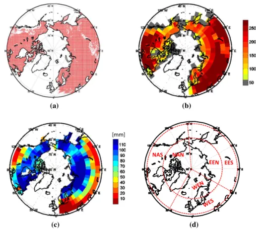
2014). The GlobSnow dataset provides monthly time series of SWE for the Northern Hemisphere land surface, exclud-ing mountainous regions, glaciers, and Greenland, at a spa-tial resolution of 25 km (Fig. 1a). Luojus et al. (2011) eval-uated the monthly GlobSnow SWE product by comparing it to ground observations from 1264 former Soviet Union and Russian stations for the 1979–2000 period, and they report good agreement with a root mean squared error of 32.8 mm for SWE values ranging between 0 and 150 mm. Li et al. (2014) compared the monthly GlobSnow and NSIDC SWE products to ground observations from 7388 Global Histori-cal Climatology Network-Daily (GHCN-DAILY) weather stations and reported much better accuracy of GlobSnow dataset than NSIDS for SWE values ranging between 30 and 200 mm. However, GlobSnow SWE generally showed underestimation in the above two studies, for SWE larger than 100 mm, as the passive microwave SWE retrieval algorithms do not have the ability to detect deep snow. In this study, we focus on the landmass north of 45°N, as it is predominantly snow covered until the end of April.

A reference grid of 5° × 5° resolution covering the Northern Hemisphere is established to facilitate the assess-ment. Monthly SWE series for each grid cell of this ref-erence grid is obtained by averaging monthly SWE series of the 25 km resolution pixels within the grid cell, for the 1980–2012 period. The number of pixels is different for each grid cell, based on the location and area of the grid cell (see Fig. 1b). This study considers land grid cells with more than 60 pixels for the analysis. Figure 1c shows mean February–April SWE for the 1980–2012 period for the grid cells included in this assessment.

Large regions encompassing several reference grid cells, from hemispheric scale to sub-continental scales, are defined for the analysis. The hemispheric scale region covers all land points north of 45°N, and will be referred to as region (A). Two sub-hemispheric scale regions are defined: southern (S) region, between 45°N–60°N and

northern (N) region between 60°N–90°N. Three continen-tal scale regions are defined: West Eurasia (WE) between 45°N–90°N and 30°W–60°E, East Eurasia (EE), covering area enclosed by 45°N–90°N and 60°E–175°W, and North America (NA) covering 45°N–90°N and 175°W–30°W. Three southern sub-continental (WES, EES, and NAS) and three corresponding northern sub-continental (WEN, EEN, and NAN) regions are defined within the three continental regions (see Fig. 1d). These continental and sub-continen-tal regions are defined following Wan et al. (2015). The monthly SWE series representing each region is then pre-pared by area-weighted averaging of the monthly series of grid cells that fall within the respective region.

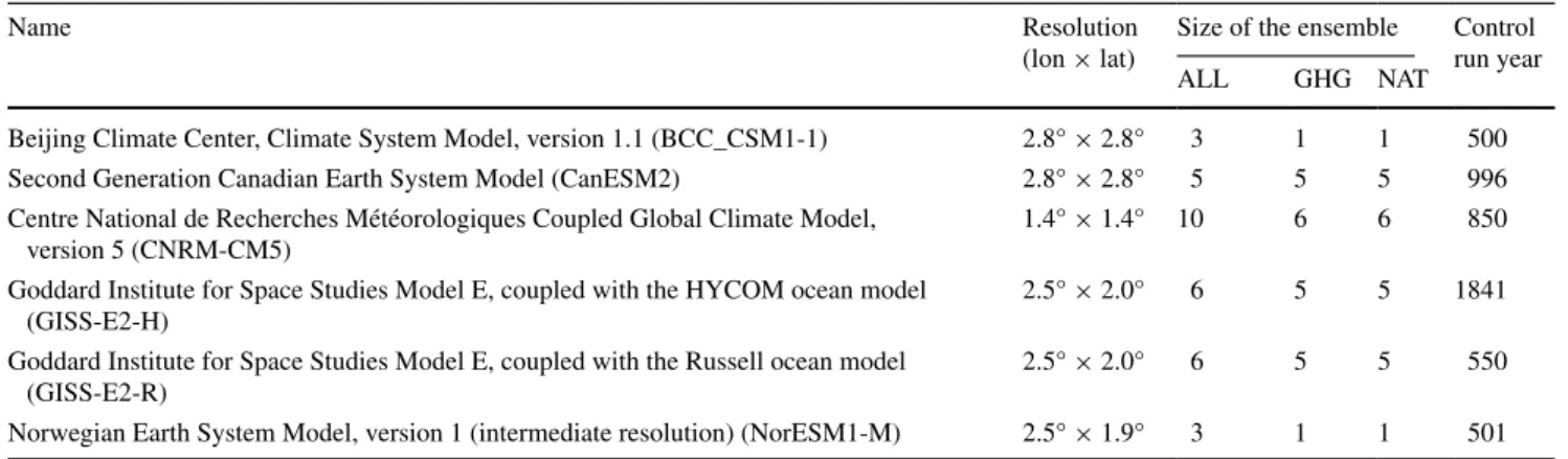
Temporal evolutions of temperature and precipitation are also evaluated for the reference domain land points for the 1980–2012 period, to investigate the effects of these parameters on SWE changes. Gridded monthly anomalies of temperature for the 5° × 5° reference resolution are directly obtained from the Climatic Research Unit (CRU) CRUTEP3 dataset (Brohan et al. 2006). Gridded monthly precipitation is obtained from the 1° × 1° resolution Global Precipitation Climatology Centre (GPCC) dataset (Schnei-der et al. 2014) and up-scaled to the 5° × 5° reference grid. Simulated SWE datasets are obtained from CMIP5 multi-model ensemble (Taylor et al. 2012). Many CMIP5 models provide historical simulation outputs from 1850 to 2005. This study employs six CMIP5 models (Table 1),

which provide simulation outputs untill 2012, to maximize record length for the D–A analysis. From the six CMIP5 models, the following ensembles are considered in this study: 33 simulations with all major anthropogenic and natural forcings (ALL; ‘historical’ experiment), 23 simu-lations of greenhouse gas forcing only (GHG; ‘historical-GHG’ experiment), and 23 simulations of natural forcing only (NAT; ‘historicalNat’ experiment). Unforced control simulation (CTL; ‘piControl’ experiment) of 3000 years length is prepared by obtaining 500 years of CTL simula-tions from each CMIP5 model. Since the six CMIP5 mod-els have different spatial resolutions (Table 1), monthly series of SWE are prepared by using the same procedures applied to the GlobSnow SWE dataset. Temporally filtered (i.e., 3 year mean area-averaged) SWE anomaly time series for CMIP5 and observations are then prepared for the 12 different regions discussed earlier for the D–A analysis.

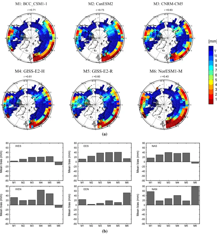
Figure 2a presents the ensemble mean of February–April SWE for the six CMIP5 models, for the ALL forcing case for the 1980–2012 period. The six CMIP5 models simulate the observed spatial pattern with spatial correlation coeffi-cients with observation in the 0.43 to 0.73 range. Among the six CMIP5 models, CanESM2 and NorESM1-M yield the highest and the lowest spatial correlation coefficients, respectively, with observation. The six CMIP5 models gen-erally overestimate SWE for all sub-continental regions, expect for NorESM1-M for the ‘WES’, ‘NAS’, and ‘WEN’

Fig. 1 a Spatial distribution of GlobSnow pixels (red dots), b the number of GlobSnow pixels for the gridcells of the 5° × 5° resolution reference domain, and c February–April GlobSnow SWE means (mm) for the 1980–2012 period on the reference gird. The six sub-continental regions defined for analysis are presented in (d)

(a) (b)

(c) (d)

NAS NAN

EES [mm]

regions, explaining the lowest spatial correlation of this model with observation. Models generally yield large posi-tive biases for northern sub-continental regions, such as GISS-E2-H and GISS-E2-R for ‘WEN’ and BCC_CSM1-1 and NorESM1-M for ‘NAN’.

3 Methodology

Linear trends (decrease/increase) in spring SWE, tempera-ture, and precipitation are investigated by using simple linear regression analysis with the ordinary least squares. The linear trends and their statistical significances at the two-tailed 90 % confidence level are estimated based on the t-statistics at the reference grid-cell and the regional scales.

The optimal fingerprinting D–A approach discussed in Allen and Stott (2003), Min et al. (2008) and Zhang et al. (2013) is used in this study. In this approach, the tempo-rally filtered version of observation y is regressed against the simulated response patterns to the externally forced sig-nals X with internal variability ε: y = Xβ + ε. The scal-ing factors (β) are estimated for the signals X prepared from both multi-model ensemble means and single-model ensemble means obtained from the six CMIP5 model simu-lations. It is well-known that the multi-model ensemble generally gives more robust detection results than a sin-gle model (Gillett et al. 2002), which is investigated with respect to spring SWE changes in this study. Residual consistency test is used to evaluate modeled internal vari-ability. The uncertainty ranges of the scaling factors can be assessed by the internal variability ε, estimated from the long CLT simulation with no variations in external forcing and the empirical orthogonal functions (EOFs) are gener-ally used to reduce the dimension of the data and improve the estimate of internal climate variability (Allen and Tett

1999; Ribes et al. 2013). In this study, the scaling factors β and their uncertainty are estimated by the total least squares

method and the residual consistency test based on the regu-larized optimal fingerprinting (ROF) technique, which can produce better results than the standard EOF approach in a mean square error sense, by using a specific estimate of the covariance matrix of the internal climate variability ε instead of decreasing the dimension by the EOFs (Ribes et al. 2013). Observed change is argued to be attributed in part to the external forcing when the 5–95 % confidence range of the scaling factor includes unity and excludes zero, as the observed and simulated changes are consist-ent in magnitude (Min et al. 2008; Zhang et al. 2013). We conduct single-signal analysis by regressing observation against simulated SWE for the ALL, GHG, and NAT cases for the multi-model and single-model ensemble means.

4 Results

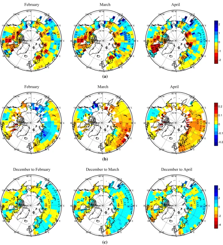
The linear trends of observed SWEs, presented in Fig. 3a for the February, March, and April months, display large spatial variability and also show differences among the defined sub-regions. Grids located in the eastern part of the ‘NAS’ and ‘NAN’ regions show statistically signifi-cant decreasing trends for SWE, which are mainly due to increasing temperatures for the same months (Fig. 3b) and/ or decreasing cumulative precipitation from the Decem-ber to spring months (Fig. 3c). Grids located in the ‘WES’ and ‘WEN’ regions generally exhibit decreasing trends for SWE, which are again generally due to the increasing tem-peratures for the same months, although some increases in cumulative precipitation from the previous December to spring months can be noted. On the contrary, many grids located in the region ‘EES’ and few grids located in the region ‘EEN’ produce statistically significant increasing trends for SWE, which could be due to significant increases in the cumulative precipitation from the previous winter to spring months (Fig. 3c). Peng et al. (2010) and Cohen et al.

Table 1 CMIP5 models used in this study

Name Resolution

(lon × lat)

Size of the ensemble Control run year

ALL GHG NAT

Beijing Climate Center, Climate System Model, version 1.1 (BCC_CSM1-1) 2.8° × 2.8° 3 1 1 500

Second Generation Canadian Earth System Model (CanESM2) 2.8° × 2.8° 5 5 5 996

Centre National de Recherches Météorologiques Coupled Global Climate Model, version 5 (CNRM-CM5)

1.4° × 1.4° 10 6 6 850

Goddard Institute for Space Studies Model E, coupled with the HYCOM ocean model (GISS-E2-H)

2.5° × 2.0° 6 5 5 1841

Goddard Institute for Space Studies Model E, coupled with the Russell ocean model (GISS-E2-R)

2.5° × 2.0° 6 5 5 550

(2012; 2014) reported an increase in mean winter (Decem-ber–February) snow depth and a decrease in winter tem-perature for the ‘EE’ region during the recent two or three decades. Changes in storm track, jet stream, and planetary waves, and their associated energy propagation induced by recent Arctic warming have been suspected as a main cause

for widespread winter cooling for this region (Cohen et al.

2012, 2014).

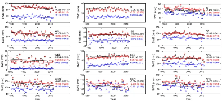
Observed SWE for the hemispherical to the sub-con-tinental scale regions shows overall decreasing trends for the 1980–2012 period, except for the regions ‘EE’ and ‘EES’ (Fig. 4). Statistically significant decreasing trends

M1: BCC_CSM1-1 M2: CanESM2 M3: CNRM-CM5

[mm]

M4: GISS-E2-H M5: GISS-E2-R M6: NorESM1-M

(b) (a)

Fig. 2 a Ensemble averages of February–April mean SWE for the six CMIP5 models (i.e., M1–M6) based on ALL forcing run for the 1980–2012 period. Spatial correlation coefficients (r) with

observa-tions (shown in Fig. 1c) are provided at the top of each panel. Mean biases in SWE when compared to GlobSnow for all sub-continental regions, for the six models, are shown in (b)

are observed for the regions ‘A’, ‘N’, ‘WE’, ‘NA’, ‘WEN’, and ‘NAN’ for February, for regions ‘N’ and ‘NAN’ for March, and for regions ‘N’, ‘NA’ and ‘NAS’ for April, at the 90 % confidence level (i.e., p value of the two-tailed test is smaller than 0.1). Spring SWE for the region ‘EES’,

however, displays statistically significant positive trends at the 90 % confidence level, which also results in weak upward trends for the region ‘EE’, particularly for March and April. The general decrease in the spring month SWE noted here is consistent with previous studies (Takala et al.

(a)

(b)

(c)

February March April

February March April

December to February December to March December to April

Fig. 3 Linear trends for the February–April months for a SWE (mm/ year) and b mean temperatures (o_{C/year), and c cumulative}

precipita-tion (mm/year) for the December to the February–April months for

the 1980–2012 period. Grid boxes with statistically significant lin-ear trends at the 90 % confidence level (two-tailed test) are indicated using the ‘ + ’ symbol

2011; Luojus et al. 2011; Li et al. 2014) at both hemi-spheric and sub-continental scales. The increase in spring SWE, for the southern part of East Eurasia, during the last few decades is also consistent with the results of Bulygina et al. (2009, 2011) based on 820 meteorological station data and those of Wu et al. (2014) based on satellite-based passive radiometer data SSM/I.

Linear trends of the spring SWE estimated from the ensemble mean signal of multi-model and each CMIP5 model for the ALL forcing case are presented in Fig. 5. The CMIP5 models generally reproduce the observed decreas-ing trends for the ‘NA’ and ‘WE’ regions and the observed increasing trends in some eastern parts of the ‘EES’ and western parts of the ‘WEN’ regions. The models, however, indicate significant decreasing trends for the western part of the region ‘EES’, where the observation yielded some increasing trends. They also show increasing trends for the ‘EEN’ and ‘NAN’ regions, where the observation generally yielded decreasing trends. All six CMIP5 models generally show large mean biases for the ‘EES’, ‘WEN’, and ‘NAN’ regions (Fig. 2b). However, NorESM1-M reproduces well the observed temporal tendency of the spring month SWEs, especially for regions ‘EEN’ and ‘NAN’, although it yielded the lowest spatial correlation coefficient and large mean biases when compared with observations for the spring SWE amounts as shown in Fig. 2.

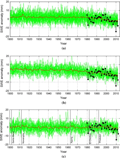
Prior to applying the D–A analysis for the spring (Feb-ruary–April average) SWE changes, the simulated sig-nals for the three different forcings (i.e., ALL, GHG, and NAT) are compared with observations. Figure 6 presents annual series of spring SWE anomalies for observation and

simulations for all three forcing cases, for region ‘A’. The anomalies observed and modelled for ALL and GHG cases show a clear decreasing trend for the last three decades. However, the multi-model ensemble mean displays smaller inter-annual variability than observation and also individual ensemble member signals. Low temporal coherence among the individual runs, induced by the diversity of the CMIP5 model physics and structures and initial conditions, can result in small inter-annual variability of the multi-model ensemble mean (Jeong and Kim 2009). The spring SWE anomalies simulated by the CMIP5 models based on the NAT forcing do not show any decreasing trend (Fig. 6c). However, effects of volcanic eruptions are reflected in the SWE anomalies. For instance, the spring SWE anomalies of both observation and simulations based on NAT forc-ing show a small increase for few years after 1992 as a response to the Pinatubo eruption, which was also noted by observed Rupp et al. (2013) in their study, but for SCE.

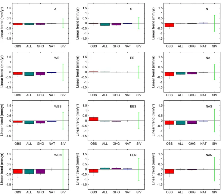
Linear trends and their 5–95 % confidence intervals of the spring SWE anomalies estimated from multi-model ensemble mean signals, for the three different cases (ALL, NAT, and GHG) are compared to those from observations for the 12 different regions for the 1980–2012 period in Fig. 7. The multi-model ensemble mean signal for ALL forcing reproduces the observed decreasing trend for the hemispheric-scale region ‘A’, while larger differences are noted for the sub-hemispheric scale regions ‘S’ and ‘N’. As shown in Figs. 2 and 5, the multi-model ensemble mean with ALL forcing fails to reproduce the statistically sig-nificant decreasing trends for regions ‘EEN’ and ‘NAN’, which results in the misrepresentation of the observed

Fig. 4 Annual time series of SWE and their trend lines for the 12 different regions for February (black), March (red) and April (blue). Estimated linear trends (mm/year) and their p values based on the two-tailed test are provided in the figures for the 3 months

February March April

[

]

decreasing trend for region ‘N’. The multi-model ensemble mean also fails to reproduce the observed statistically sig-nificant increasing trend for the region ‘EES’, which results in an overestimation of the observed decreasing trend for region ‘S’. However, the multi-model ensemble mean reproduces well the observed decreasing trends for other regions. The multi-model ensemble mean with GHG forc-ing displays a very similar pattern to that with ALL forcforc-ing,

implying that the GHG forcing is the main external forcing of the spring SWE changes in the CMIP5 model simula-tions. The 5–95 % confidence intervals of the linear trends of the multi-model ensemble mean based on ALL and GHG forcings are much smaller than those for the observa-tion for all regions, implying that the inter-annual variabil-ity of the multi-model ensemble mean is smaller than that observed. The multi-model ensemble mean based on NAT forcing produces statistically insignificant small trends for all regions. The internal variability estimated from the CTL simulations (column 5 of Fig. 7) is higher for the region ‘N’ compared to the region ‘S’ and similarly increase with decreasing area. The regions, which have large internal variability, generally yield large confidence intervals for

Fig. 6 Observed and simu-lated spring (February–April average) SWE anomalies at the hemispheric scale region ‘A’ from the 1980–2010 baseline period based on a all major anthropogenic and natural (ALL) forcing, b greenhouse gas (GHG) forcing only, and c natural (NAT) forcing only. The black dots are observations. The green lines (33, 23 and 23 respectively for the ALL, GHG, and NAT cases) are SWE anomalies from the six CMIP5 models considered in this study. The thick red lines are the full ensemble average. Major vol-canic eruptions are presented in (c) as vertical gray lines

Pinatubo El Chicho n Agung Novarupt a Santa Mari a (a) (b) (c) Fig. 5 Linear trends in SWE estimated from ensemble means of

multi-model and individual CMIP5 models based on ALL forcing for the February–April months for the 1980–2012 period. Grid boxes with statistically significant linear trends at the 90 % confidence level (two-tailed test) are indicated using the ‘ + ’ symbbol. Red and blue contours enclose regions where linear trends of simulations are 1 mm/year larger and smaller, respectively, than those of observation

the linear trends for both observation and the multi-model ensemble.

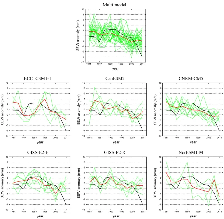
Figure 8 shows the temporally smoothed time series of spring SWE anomalies observed and modelled (for ALL), for the hemisphere scale region ‘A’. The smoothed observa-tion shows a significant downward trend particularly after 1996 and an important decreasing for the last 6 years. The individual signals obtained from the six CMIP5 models also suggest a decreasing trend for the SWE anomalies. The multi-model ensemble mean of the 33 ALL forcing runs reproduces the observed decreasing trend, though it dis-plays smaller temporal variability compared to both obser-vation and individual ensemble members. The individual

CMIP5 models reproduce the observed decreasing trend in the smoothed observation to varying degrees. BCC_CSM1-1, CNRM-CM5, GISS-E2-H, and NorESM1-M repro-duce the temporal variability of the smoothed observation relatively well, compared to CanESM2 and GISS-E2-R in terms of Pearson’s linear correlation coefficient. Ensem-ble means of the individual models tend to exhibit larger variance than the multi-model ensemble mean. However, ensemble means of individual CMIP5 models yield lower linear correlation coefficients with observations than the multi-model ensemble mean.

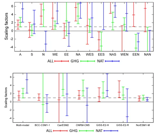
Figure 9 shows scaling factors and their 5–95 % con-fidence ranges estimated by the D–A analysis of the

Fig. 7 Spring SWE linear trends and their 5–95 % confidence inter-vals for observations and multi-model ensemble mean signals simu-lated by the six CMIP5 models based on the three different forcings for the 12 different regions for the 1980–2012 period. Green error

bar in column 5 represents the 1-sigma (15.9–84.1 %) range of the standardized internal variability (SIV) noise estimated from control simulations (unit: m/m)

multi-model ensemble mean signals for the three forcing cases for the 12 different regions. The scaling factors of both ALL and GHG forcings are significantly greater than zero for the hemispheric scale region ‘A’, indicating that the combined effects of external anthropogenic and natu-ral forcings or the effect of GHG forcing alone are detected in spring SWE decline for the landmass north of 45°N. Moreover, the 5–95 % confidence ranges of the scaling fac-tors include unity, indicating that the simulated signals of

the spring SWE decreases under the ALL and GHG forc-ings are consistent with the observed spring SWE decrease at the hemisphere-scale. However, detection and attribu-tion of ALL and GHG forcings to spring SWE changes are less clear for the smaller regions. Scaling factors of both ALL and GHG forcings are statistically significant for the regions ‘N’, ‘WE’, ‘NA’, and ‘NAS’. However, some of them (i.e., scaling factors for regions ‘N’, ‘NA’, and ‘NAS’ for ALL and regions ‘N’ and ‘NA’ for GHG) indicate that Multi-model

BCC_CSM1-1 CanESM2 CNRM-CM5

GISS-E2-H GISS-E2-R NorESM1-M

Fig. 8 Time series of 3 year mean area-averaged spring SWE anoma-lies for observations and CMIP5 models for the ALL forcing case for the hemisphere scale region ‘A’ for the 1981–2012 period. Green, red,

and black lines represent the individual simulations, their ensemble average, and observations, respectively

the simulated signals of the CMIP5 models, as a group, are not consistent with observations and tend to underes-timate the spring SWE response to external forcings due to improper reproduction of temporal variability of indi-vidual models, as their 5–95 % confidence ranges do not include unity. The observed decreasing trends of spring SWE were reproduced properly by multi-model ensemble signals at the sub-continental regions ‘WES’, ‘WEN’, and ‘NAS’ (Fig. 7). However, the combined effect of ALL forc-ing or GHG forcforc-ing alone are not detected clearly by the D–A analysis, indicating that the observed and simulated spring SWE changes have large noise range, which makes it difficult to detect signals outside the noise range for the small sub-continental scale regions. Scaling factors and their 5–95 % confidence ranges of the NAT forcing only are much larger than unity for the regions ‘A’, ‘WE’, ‘NA’, and ‘NAS’, include zero for regions ‘EE’, ‘WES’, ‘WEN’, and ‘NAN’, and is negative for regions ‘N’, and ‘EEN’, indicating that the effect of NAT forcing alone are gener-ally undetectable or inconsistent with the observed spring SWE changes for the considered regions.

Figure 10 compares best estimates of scaling factors and their 5–95 % confidence ranges for the multi-model ensem-ble mean and that of single-model ensemensem-ble means for the hemispheric scale region ‘A’. The effects of ALL and GHG forcings are generally detected by most individual model simulations, except for BCC_CSM1-1 for GHG forcing

and CanESM2 for ALL forcing. The single-model ensem-bles, however, tend to produce larger 5–95 % confidence ranges of scaling factors for the ALL and GHG forcings compared to the multi-model ensemble, except NorESM1-M, supporting robustness of the detection results from multi-model ensemble mean. This result roughly implies that individual models usually have larger uncertainty in the estimation of SWE responses (fingerprints) (as shown in Fig. 8) and, therefore, the detection and attribution analysis based on the multi-model could provide more robust results than individual models, which has also been reported through the D–A analyses for the global surface temperature (Gillett et al. 2002) and Northern Hemisphere spring SCE (Rupp et al. 2013).

5 Summary and discussion

This study investigated spring (February–April) snow water equivalent (SWE) changes using the GlobSnow observation dataset for the 1980–2012 period, for different regions at local (5° × 5° resolution) to hemispheric (higher than 45°N) scales over the Northern Hemisphere land-points. Consequently, this study provided spatially more comprehensive information about the spring SWE changes over the Northern Hemisphere, compared to previous sim-ilar studies (i.e., Brown 2000; Luojus et al. 2011; Takala

Fig. 9 Best estimates (data points) and 5–95 % confidence intervals (error bars) of the scaling factors for spring SWE estimated from the multi-model ensemble signals simulated by six CMIP5 models based on ALL, GHG, and NAT forcings for the 12 different regions

Fig. 10 Best estimates (data points) and 5–95 % confidence interval (error bars) of the scaling factors of spring SWE estimated from the multi-model ensemble signals and single-model ensemble signals based on ALL, GHG, and NAT forc-ings for the hemispheric scale region ‘A’

et al. 2011; Gen et al. 2013; Li et al. 2014) which mainly focused on hemispheric and/or continental scale, although these studies were not directly comparable with this study as their analysis periods and snow characteristics were dif-ferent from those of this study. Results suggest statistically significant decreasing trends in spring SWE for the east-ern parts of North America and West Eurasia, mainly due to increasing trends in the spring temperatures, as reported in previous studies. However, remarkable increasing trends were observed for the southern part of east Eurasia, mainly due to significant increases in accumulated precipitation from the previous winter to spring period. The increases in spring SWE for east Eurasia for the last few decades are consistent with the findings by Bulygina et al. (2009, 2011) and Wu et al. (2014), based on spring SCE and/or SWE.

This study applied the detection–attribution (D–A) approach to demonstrate the anthropogenic and natu-ral effects on the spring SWE changes, by comparing the observations to six CMIP5 model simulations for different regions at sub-continental to hemispheric scales over the Northern Hemisphere. Six CMIP5 models with all major anthropogenic and natural (ALL) forcings reproduced the spatial distribution of observed spring SWE fairly well over the study area. They also reproduced properly temporal decreasing trends of observed spring SWE for West Eura-sia and North America. The models, however, showed some difficulty in reproducing observed spring SWE changes for sub-continental scales such as southern and northern parts of East Eurasia and northern part of North America. Multi-model ensemble mean of the six CMIP5 Multi-models with only greenhouse gas (GHG) forcing produced very similar trends to those with ALL forcing for the spring SWE changes, indicating that the temporal changes are mainly induced by the well mixed GHG forcing rather than the other anthropo-genic (OANT) forcings and/or natural forcings for the anal-ysis period. This is consistent with the study by Najafi et al. (2015), which reported little changes in the response of the mean annual Arctic temperature anomalies to OANT for the 1980–2010 period. It must be noted though that the main control on February–April SWE is the spring temperature.

The D–A assessment suggests that multi-model ensem-ble mean signals based on the combined effects of external anthropogenic and natural forcings and the effect of GHG forcing only are consistent with the observed spring SWE decrease over hemispheric scale landmass. However, the effects of ALL and/or GHG forcings were not detected clearly for the smaller regions. This might be due to the large temporal noise in observation and improper reproduc-tion of the temporal variability by the CMIP5 models at the scale of small regions considered in this study. Hegerl et al. (2007) and Stott et al. (2010) also discussed the limitation of the D–A analysis at regional scale caused by the relative low signal-to-noise ratios and limitations of global climate

models in capturing some characteristics of regional varia-bility. Detection and attribution results based on single mod-els for ALL and GHG forcings for spring SWE decreases show larger uncertainty compared to those based on the multi-model ensemble, at the hemispheric scale. This is due to the less coherent temporal variability of individual model signals with observations compared to that between multi-model ensemble signals and observations. The detection and attribution analysis results based on single-models com-pared to multi-model ensemble is consistent with the find-ings of Gillett et al. (2002) and Rupp et al. (2013).

The analysis period of this study is relatively short and the estimated spring SWE trends during the period can be affected by natural decadal variability such as Pacific decadal oscillation (PDO) and North Atlantic oscilla-tion (NAO) as shown in Trenberth et al. (2014) and Ding et al. (2014). Possible influence of such natural variability modes on the observed SWE changes and detection/attribu-tion results will be considered in future work. Addidetection/attribu-tionally, trend and D–A analyses based on different combinations of sub-regions such as ‘NA’-’EE’ or ‘NA’–’WE’ could be considered in future work. Two-signal analysis using both anthropogenic (ANTH = ALL–NAT) and natural forcings simultaneously could also be employed in future to identify the separate contributions of these forcings.

Acknowledgments This research was undertaken within the frame-work of the Canada Research Chair in Regional Climate Modelling. Open Access This article is distributed under the terms of the Creative Commons Attribution 4.0 International License ( http://creativecom-mons.org/licenses/by/4.0/), which permits unrestricted use, distribu-tion, and reproduction in any medium, provided you give appropriate credit to the original author(s) and the source, provide a link to the Creative Commons license, and indicate if changes were made.

References

Allen MR, Stott PA (2003) Estimating signal amplitudes in optimal fingerprinting, part I: theory. Clim Dyn 21(5–6):477–491 Allen MR, Tett SFB (1999) Checking for model consistency in

opti-mal fingerprinting. Clim Dyn 15(6):419–434

Armstrong RL, Brodzik MJ (2001) Recent Northern Hemi-sphere snow extent: a comparison of data derived from vis-ible and microwave satellite sensors. Geophys Res Lett 28(19):3673–3676

Barnett T, Adam J, Lettenmaier D (2005) Potential impacts of a warming climate on water availability in snow-dominated regions. Nature 438:303–309

Bednorz E (2004) Snow cover in eastern Europe in relation to tem-perature, precipitation and circulation. Int J Climatol 24:591–601 Bindoff NL, Stott PA, AchutaRao KM, Allen MR, Gillett N, Gutzler

D, Hansingo K, Hegerl GC, Hu Y, Jain S, Mokhov II, Overland J, Perlwitz J, Sebbari R, Zhang X (2013) Detection and attribution of climate change: from global to regional. In: Stocker TF, Qin D, Plattner G-K, Tignor M, Allen SK, Boschung J, Nauels A, Xia Y, Bex V, Midgley PM (eds) Climate change 2013: the physical

science basis. Contribution of working group I to the fifth assess-ment report of the intergovernassess-mental panel on climate change. Cambridge University Press, Cambridge, New York

Brohan P, Kennedy JJ, Harris I, Tett SFB, Jones PD (2006) Uncer-tainty estimates in regional and global observed temperature changes: a new data set from 1850. J Geophys Res 111:D12106. doi:10.1029/2005JD006548

Brown RD (2000) Northern hemisphere snow cover variability and change, 1915–97. J Clim 13(13):2339–2355

Brown RD, Robinson DA (2011) Northern Hemisphere spring snow cover variability and change over 1922–2010 including an assessment of uncertainty. Cryosphere 5:219–229. doi:10.5194/tc-5-219-2011

Brown R, Derksen C, Wang L (2010) A multi-data set analysis of variability and change in Arctic spring snow cover extent, 1967– 2008. J Geophys Res 115:D16111. doi:10.1029/2010JD013975

Bulygina ON, Razuvaev VN, Korshunova NN (2009) Changes in snow cover over Northern Eurasia in the last few decades. Envi-ron Res Lett 4(4):045026

Cohen JL, Furtado JC, Barlow MA, Alexeev VA, Cherry JE (2012) Arctic warming, increasing snow cover and widespread boreal winter cooling. Environ Res Lett 7(1):014007

Cohen J, Screen JA, Furtado JC, Barlow M, Whittleston D, Cou-mou D, Francis J, Dethloff K, Entekhabi D, Overland J, Jones J (2014) Recent Arctic amplification and extreme mid-latitude weather. Nat Geosci 7(9):627–637

Ding Q, Wallace JM, Battisti DS, Steig EJ, Gallant AJ, Kim HJ, Geng L (2014) Tropical forcing of the recent rapid Arctic warming in northeastern Canada and Greenland. Nature 509(7499):209–212 Egli L, Jonas T, Meister R (2009) Comparison of different automatic

methods for estimating snow water equivalent. Cold Reg Sci Technol 57(2):107–115

ESA (2014) The third GlobSnow-2 newsletter gives an overview of the GlobSnow-2 SE and SWE v2.0 datasets released mid-December 2013. (http://www.globsnow.info/index.php?page=Newsletters) Gan TY, Barry RG, Gizaw M, Gobena A, Balaji R (2013) Changes

in North American snowpacks for 1979–2007 detected from the snow water equivalent data of SMMR and SSM/I passive microwave and related climatic factors. J Geophys Res Atmos 118:7682–7697

Gillett NP, Zwiers FW, Weaver AJ, Hegerl GC, Allen MR, Stott PA (2002) Detecting anthropogenic influence with a multi-model ensemble. Geophys Res Lett 29(20):1970. doi:10.1029/2002GL015836

Gong G, Entekhabi D, Cohen J, Robinson D (2004) Sensitivity of atmospheric response to modeled snow anomaly characteristics. J Geophys Res 109:D06107. doi:10.1029/2003JD004160

Hancock S, Baxter R, Evans J, Huntley B (2013) Evaluating global snow water equivalent products for testing land surface models. Remote Sens Environ 128:107–117

Hegerl GC, Zwiers F (2011) Use of models in detection and attri-bution of climate change. WIREs Clim Change 2:570–591. doi:10.1002/wcc.121

Hegerl GC, Crowley TJ, Allen M, Hyde WT, Pollack HN, Smerdon J, Zorita E (2007) Detection of human influence on a new, vali-dated 1500-year temperature reconstruction. J Clim 20:650–666. doi:10.1175/JCLI4011.1

IPCC (2013) Climate change 2013: the physical science basis. In: Stocker TF, Qin D, Plattner G-K, Tignor M, Allen SK, Boschung J, Nauels A, Xia Y, Bex V, Midgley PM (eds) Contribution of working group I to the fifth assessment report of the intergov-ernmental panel on climate change. Cambridge University Press, Cambridge, New York

Jeong DI, Kim Y-O (2009) Combining single-value streamflow fore-casts—a review and guidelines for selecting techniques. J Hydrol 377(3):284–299

Lemke P, Ren J, Alley RB, Allison I, Carrasco J, Flato G, Fujii Y, Kaser G, Mote P, Thomas RH, Zhang T (2007) Observations:

changes in snow, ice and frozen ground. In: Solomon S, Qin D, Manning M, Chen Z, Marquis M, Averyt KB, Tignor M, Miller HL (eds) Climate change 2007: the physical science basis Con-tribution of working group I to the fourth assessment report of the intergovernmental panel on climate change. Cambridge Uni-versity Press, Cambridge, New York

Li Z, Liu J, Huang L, Wang N, Tian B, Zhou J, Chen Q, Zhang P (2014) Snow mass decrease in the Northern Hemisphere (1979/80–2010/11). The Cryosphere Discuss 8:5623–5644. doi:10.5194/tcd-8-5623-2014

Luojus K, Pulliainen J, Takala M, Lemmetyinen J, Derksen C, Met-samaki S, Bojkov B (2011) Investigating hemispherical trends in snow accumulation using GlobSnow snow water equivalent data. In Geoscience and remote sensing symposium (IGARSS), 2011 IEEE international, pp 3772–3774. IEEE

Min SK, Zhang X, Zwiers FW, Agnew T (2008) Human influence on Arctic sea ice detectable from early 1990s onwards. Geophys Res Lett. doi:10.1029/2008GL035725

Najafi MR, Zwiers FW, Gillett NP (2015) Attribution of Arctic tem-perature change to greenhouse-gas and aerosol influence. Nat Clim Change 5:246–249. doi:10.1038/nclimate2524

Peng S, Piao S, Ciais P, Fang J, Wang X (2010) Change in winter snow depth and its impacts on vegetation in China. Glob Change Biol 16(11):3004–3013

Pierce DW, Barnett TP, Hidalgo HG, Das T, Bonfils C, Santer BD, Bala G, Dettinger MD, Cayan DR, Mirin A, Wood AW, Nozawa T (2008) Attribution of declining Western U.S. snowpack to human effects. J Clim 21:6425–6444

Pulliainen J (2006) Mapping of snow water equivalent and snow depth in boreal and sub-arctic zones by assimilating space-borne microwave radiometer data and ground-based observations. Remote Sens Environ 101(2):257–269

Ribes A, Planton S, Terray L (2013) Application of regularised opti-mal fingerprinting to attribution. Part I: method, properties and idealised analysis. Clim Dyn 41(11–12):2817–2836

Rupp DE, Mote PW, Bindoff NL, Stott PA, Robinson DA (2013) Detection and attribution of observed changes in Northern Hemi-sphere spring snow cover. J Clim 26(18):6904–6914

Schneider U, Becker A, Finger P, Meyer-Christoffer A, Ziese M, Rudolf B (2014) GPCC’s new land surface precipitation cli-matology based on quality-controlled in situ data and its role in quantifying the global water cycle. Theor Appl Climatol 115:15–40

Stott PA, Gillett NP, Hegerl GC, Karoly DJ, Stone DA, Zhang X, Zwiers F (2010) Detection and attribution of climate change: a regional perspective. WIREs Clim Change 1:192–211. doi:10.1002/wcc.34

Takala M, Luojus K, Pulliainen J, Derksen C, Lemmetyinen J, Kärnä JP, Koskinen J, Bojkov B (2011) Estimating northern hemisphere snow water equivalent for climate research through assimilation of space-borne radiometer data and ground-based measurements. Remote Sens Environ 115(12):3517–3529

Taylor KE, Stouffer RJ, Meehl GA (2012) An overview of CMIP5 and the experiment design. Bull Am Meteor Soc 93:485–498 Trenberth KE, Fasullo JT, Branstator G, Phillips AS (2014) Seasonal

aspects of the recent pause in surface warming. Nat Clim Change 4(10):911–916

Wan H, Zhang X, Zwiers F, Min SK (2015) Attributing northern high-latitude precipitation change over the period 1966–2005 to human influence. Clim Dyn 45(7–8):1713–1726

Wu R, Liu G, Ping Z (2014) Contrasting Eurasian spring and sum-mer climate anomalies associated with western and eastern Eurasian spring snow cover changes. J Geophys Res Atmos 119:7410–7424

Zhang X, Wan H, Zwiers FW, Hegerl GC, Min SK (2013) Attribut-ing intensification of precipitation extremes to human influence. Geophys Res Lett 40(19):5252–5257