HAL Id: inria-00506591
https://hal.inria.fr/inria-00506591
Submitted on 28 Jul 2010HAL is a multi-disciplinary open access archive for the deposit and dissemination of sci-entific research documents, whether they are pub-lished or not. The documents may come from teaching and research institutions in France or abroad, or from public or private research centers.
L’archive ouverte pluridisciplinaire HAL, est destinée au dépôt et à la diffusion de documents scientifiques de niveau recherche, publiés ou non, émanant des établissements d’enseignement et de recherche français ou étrangers, des laboratoires publics ou privés.
Bayesian numerical inference for Markovian models –
Application to tropical forest dynamics
Fabien Campillo, R. Rakotozafy, Vivien Rossi
To cite this version:
Fabien Campillo, R. Rakotozafy, Vivien Rossi. Bayesian numerical inference for Markovian models – Application to tropical forest dynamics. International Conference on Approximation Methods and Numerical Modelling in Environment and Natural Resources, Jul 2007, Granada, Spain. pp.53-56. �inria-00506591�
Granada (Spain), July 11-13, 2007
Bayesian numerical inference for markovian models.
Application to tropical forest dynamics.
Fabien Campillo1, Rivo Rakotozafy2and Vivien Rossi3
1INRIA/IRISA
Campus de Beaulieu, 35042 Rennes Cedex, France e-mail: [email protected]
2University of Fianarantsoa
BP 1264, Andrainjato, 301 Fianarantsoa, Madagascar e-mail: [email protected]
3CIRAD
Campus International de Baillarguet, 34398 Montpellier cedex 5, France e-mail: [email protected]
Keywords: Markov chain Monte Carlo method, interacting chains, hidden Markov model,
forest dynamic model
Abstract. Bayesian modelling is fluently employed to assess natural ressources. It is associated
with Monte Carlo Markov Chains (MCMC) to get an approximation of the distribution law of interest. Hence in such situations it is important to be able to proposeN independent realiza-tions of this distribution law. We propose a strategy for makingN parallel Monte Carlo Markov Chains interact in order to get an approximation of an independentN-sample of a given target law. In this method each individual chain proposes candidates for all other chains. We prove that the set of interacting chains is itself a MCMC method for the product ofN target measures. Compared to independent parallel chains this method is more time consuming, but we show through example that it possesses many advantages. This approach will be applied to a forest dynamic model.
1
Introduction
In many models arising in environment (ecology, population dynamics, renewable resource management etc.), measurements y1, . . . , yT are collected yearly or monthly so that the real-time
constraint is not relevant even if the underlying law features a temporal structure. State-space modeling of these data consists in proposing a Markov process (xt, yt)t=1···T, where the state
process xt is not observed and ytare the associated observation process. This process usually
depends on some unknown parameterθ with given a priori law. The goal of the Bayesian
infer-ence is to determine the a posteriori law of(x1:T, θ) given the measurements y1:T. In the case of
F. Campillo,R. Rakotozafy and V. Rossi
Bayesian inference is mainly due to the development of efficient Monte Carlo approximation techniques [6]. Among them, MCMC methods allow us to sample from almost any prescribed distribution law [3]. Still high dimensional or “tricky” distribution laws are barely tackled by these techniques and should be approached with realistic expectations. Together with numerical Bayesian inference, hidden Markov models for general state-space have been recently used in environment sciences and ecology, see e.g. [5]
MCMC algorithms [6] allow us to draw samples from a probability distribution π(x) dx
known up to a multiplicative constant. This consists in sequentially simulating a single Markov chain whose limit distribution isπ(x) dx. There exist many techniques to speed up the
conver-gence toward the target distribution by improving the mixing properties of the chain.
In practice one however can make use of several chains in parallel. It is then tempting to exchange information between these chains to improve mixing properties of the MCMC samplers. A general framework of “Population Monte Carlo” has been proposed in this context [2]. In this paper we propose an interacting method between parallel chains which provides an independent sample from the target distribution. Contrary to papers previously cited, the proposal law in our work is given and does not adapt itself to the previous simulations. Hence, the problem of the choice of the proposal law still remains.
2
Parallel/interacting Metropolis within Gibbs (MwG) algorithm
Letπ(x) be the probability density function of a target distribution defined on (IRn, B(IRn)).
Forℓ = 1, . . . , n, we define the conditional laws: πℓ(xℓ|x¬ℓ)
def
= π(x1:n)/R π(x1:n) dx¬ℓ. (1)
where¬ℓ def
= {m = 1 : n; m 6= ℓ}. When we know to sample from (1), we are able to use the
Gibbs sampler. It is possible to adapt our interacting method to parallel Gibbs sampler. But very often we do not know how to sample from (1) and therefore we consider proposal conditional densitiesπprop
ℓ (xℓ) defined for all ℓ. In this case, we use MwG algorithm.
One iterationX → Z of the parallel/interacting MwG method consists in updating the
com-ponentsXℓsuccessively forℓ = 1, . . . , n, i.e. [X1:n] → [Z1X2:n] → [Z1:2X3:n] · · · [Z1:n−1Xn] →
[Z1:n]. For each ℓ fixed, the subcomponents Xℓi are updated sequentially fori = 1 : N in two
steps:
1. Proposal step: We sample independentlyN candidates Yℓj ∈ IR according to:
Yℓj ∼ πℓ,prop i,j (ξ|JZ, X i ℓ, XK i ℓ) dξ , 1 ≤ j ≤ n whereJZ, ξ, XKi ℓ def = Z1:ℓ−1 Z1 ℓ .. . Zℓi−1 ξ Xℓi+1 .. . XN ℓ Xℓ+1:n .
We also use the following lighter notation:πℓ,prop
i,j (ξ|ξ′) = π ℓ,prop
i,j (ξ|JZ, ξ′, XKiℓ).
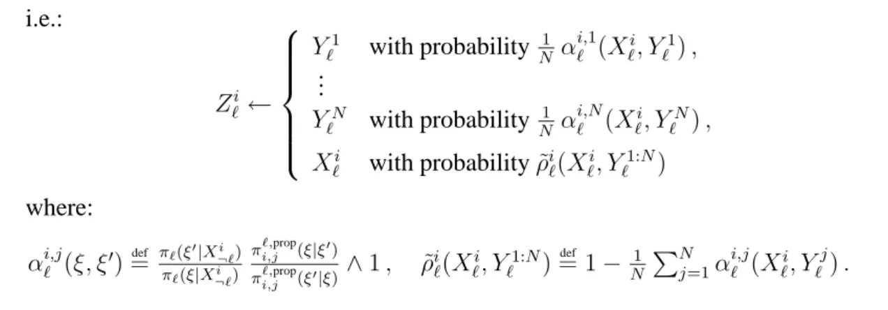
2. Selection step: The subcomponentXi
ℓcould be replaced by one of theN candidates Yℓ1:N
or stay unchanged according to a multinomial sampling, the resulting value is calledZi ℓ,
i.e.: Zi ℓ ← Y1 ℓ with probability N1 α i,1 ℓ (X i ℓ, Yℓ1) , .. . YN ℓ with probability 1 N α i,N ℓ (X i ℓ, Y N ℓ ) , Xi ℓ with probabilityρ˜iℓ(Xℓi, Yℓ1:N) where: αi,jℓ (ξ, ξ′) def = πℓ(ξ′|X¬ℓi ) πℓ(ξ|X¬ℓi ) πℓ,propi,j (ξ|ξ′) πℓ,propi,j (ξ′|ξ) ∧ 1 , ρ˜ i ℓ(Xℓi, Yℓ1:N) def = 1 − 1 N PN j=1α i,j ℓ (Xℓi, Y j ℓ) .
Proposition LetP (X, dZ) the Markov kernel on IRn×N associated with the MwG algorithm,
the measureΠ(dX) = π(X1) dX1· · · π(XN) dXN is invariant for the kernelP , i.e. ΠP = Π.
The proof is detailed in [1].
3
Numerical tests
Our aim is to show that making parallel samplers interact could speed up the convergence toward the stationary distribution.
An hidden Markov model. We apply the parallel/interacting MwG sampler to a toy problem where a good estimateπ of the target distribution π is available. Considerˆ
sℓ+1 = a sℓ+ wℓ, yℓ = b sℓ+ vℓ
for ℓ = 1 · · · n, where s1 ∼ N (¯s1, Q1), w1:n and v1:n are centered white Gaussian noises
with variances σ2
w and σ
2
v. Suppose that b is known and a = θ is unknown with a priori
lawN (µθ, σ2θ). We also suppose that w1:n, v1:n, s1 andθ are mutually independent.
The state variable is x1:n+1
def
= (s1:n, θ) and the target law is π(s1:n, ϑ) ds1:ndϑ
def
= law(s1:n, θ|y1:n=
y1:n). We will perform two algorithms: (i) N parallel/interacting MwG samplers and (ii) N
par-allel/independent MwG samplers. For methods (i) and (ii) we performN = 50 parallel samplers
so we computeǫ(i )andǫ(ii ). ǫ(·)is an indicator which must decrease and remain close to a small
value when convergence toward the stationary distribution occurs.
0 5 10 15 20 25 30 35 40 45 50 0 0.2 0.4 0.6 0.8 1 1.2 1.4 1.6 1.8 2
CPU time (sec.) L1 error estimation 0 1000 2000 3000 4000 5000 0 0.2 0.4 0.6 0.8 1 1.2 1.4 1.6 1.8 2
CPU time (sec.) L1
error estimation
Figure 1: Left: Evolution of the indicators ǫ(ii) for the parallel/independent MwG sampler (- -), and ǫ(i)for the parallel/interacting MH sampler (–). Right: Evolution of the indicator ǫ(ii) for the parallel/independent MwG sampler (- -). After 5000 sec. CPU time, the convergence of this method is still unsatisfactory.
F. Campillo,R. Rakotozafy and V. Rossi
ǫ(·) is based on theL1errors betweenˆπ and the kernel density estimates of the target density
based on the final values of method (i) or (ii) (see [1] for details).
To compare fairly the parallel/independent MwG algorithm and the parallel/interacted MwG algorithm, we represent on Figure 1 the indicatorsǫ(i)andǫ(ii )not as a function of the iteration
number of the algorithm but as a function of the CPU time. In Figure 1 (left) we see that even if one iteration of algorithm (i) needs more CPU than one of (ii), still the first algorithm converges more rapidly than the second one. This shows the inefficiency of parallel/independent MwG on this simple model.
Real case study: a tropical forest. Forest dynamics models have emerged to assess the sus-tainability of the management of tropical forest. Among various types of models, matrix models rely on a description of the forest stand by a discrete diameter distribution. The state of a tree corresponds to its belonging to a diameter class and the shifts from one class to another occur by discrete time step. Matrix model of forest dynamics rely on four hypotheses (see [4] for details) of which Markov’s hypothesis. So the parallel/interacted MwG algorithm can be used to calibrate a matrix model. An illustration on a data set obtained from experimental forest plots in a tropical rain forest of French Guiana will be presented.
4
Conclusion
This work showed that making parallel MCMC chains interact could improve their conver-gence properties. We presented the basic properties of the MCMC method, we did not prove that the proposed strategy speeds up the convergence. This difficult point is related to the prob-lem of the rate of the convergence of the MCMC algorithms. Through simple examples we saw that the MwG strategy could be a poor strategy. In this situation our strategy improved the convergence properties.
REFERENCES
[1] F. Campillo and V. Rossi. Parallel and interacting Markov chains Monte Carlo method. Research report n.6008, INRIA, (2006), 30p.
http://hal.inria.fr/inria-00103871.
[2] O. Capp´e, A. Guillin, J.-M. Marin, and C.P. Robert.Population Monte Carlo. Journal of Computational and Graphical Statistics, Vol. 13(4), (2004), pp. 907–929.
[3] W.R. Gilks, S. Richardson, and D.J. Spiegelhalter, editors.Markov Chain Monte Carlo in
practice. Chapman & Hall, London, 1995.
[4] N. Picard, A. Bar-Hen, Y. Gu´edon. Modelling diameter class distribution with a
second-order matrix model. For. Ecol. Manage., Vol. 180, (2002), pp.389-400.
[5] E. Rivot, E. Prevost, E. Parent, and J.-L. Blagini`ere. A Bayesian state-space modelling
framework for fitting a salmon stage-structured population dynamic model to multiple time series of field data. Ecological Modelling, Vol. 179, (2004), pp.463-485.
[6] C.P. Robert and G. Casella. Monte Carlo Statistical Methods. Springer–Verlag, Berlin, 2nd edition, 2004.