HAL Id: inserm-00356883
https://www.hal.inserm.fr/inserm-00356883
Submitted on 28 Jan 2009
HAL is a multi-disciplinary open access
archive for the deposit and dissemination of
sci-entific research documents, whether they are
pub-lished or not. The documents may come from
teaching and research institutions in France or
abroad, or from public or private research centers.
L’archive ouverte pluridisciplinaire HAL, est
destinée au dépôt et à la diffusion de documents
scientifiques de niveau recherche, publiés ou non,
émanant des établissements d’enseignement et de
recherche français ou étrangers, des laboratoires
publics ou privés.
Fully Bayesian joint model for MR brain scan tissue and
structure segmentation
Benoit Scherrer, Florence Forbes, Catherine Garbay, Michel Dojat
To cite this version:
Benoit Scherrer, Florence Forbes, Catherine Garbay, Michel Dojat. Fully Bayesian joint model for
MR brain scan tissue and structure segmentation. 11th International Conference on Medical Image
Computing and Computer-Assisted Intervention – MICCAI 2008, Sep 2008, New York, NY, United
States. pp.1066-1074, �10.1007/978-3-540-85990-1_128�. �inserm-00356883�
Tissue and Structure Segmentation
B. Scherrer1,3,4, F. Forbes2,4, C. Garbay3,4, M. Dojat1,4
1
INSERM, U836, Grenoble, F-38043, France
2
INRIA, MISTIS, Grenoble, France
3 CNRS, MAGMA, Grenoble, France 4
Universit´e Joseph Fourier, Grenoble, France
Abstract. In most approaches, tissue and subcortical structure segmen-tations of MR brain scans are handled globally over the entire brain volume through two relatively independent sequential steps. We propose a fully Bayesian joint model that integrates local tissue and structure segmentations and local intensity distributions. It is based on the speci-fication of three conditional Markov Random Field (MRF) models. The first two encode cooperations between tissue and structure segmentations and integrate a priori anatomical knowledge. The third model specifies a Markovian spatial prior over the model parameters that enables local estimations while ensuring their consistency, handling this way nonuni-formity of intensity without any bias field modelization. The complete joint model provides a sound theoretical framework for carrying out tis-sue and structure segmentation by distributing a set of local and coop-erative MRF models. The evaluation, using a previously affine-registred atlas of 17 structures and performed on both phantoms and real 3T brain scans, shows good results.
1
Introduction
Difficulties in automatic MR brain scan segmentation arise from various sources. The nonuniformity of image intensity results in spatial intensity variations within each tissue, which is a major obstacle to an accurate automatic tissue segmenta-tion. The automatic segmentation of subcortical structures is a challenging task as well. It cannot be performed based only on intensity distributions and requires the introduction of a priori knowledge. Most of the proposed approaches share two main characteristics. First, tissue and subcortical structure segmentations are considered as two successive tasks and treated relatively independently al-though they are clearly linked: a structure is composed of a specific tissue, and knowledge about structures locations provides valuable information about local intensity distribution for a given tissue. Second, tissue models are estimated glob-ally through the entire volume and then suffer from imperfections at a local level. Alternative local procedures exist but are either used as a preprocessing step [1] or use redundant information to ensure consistency of local models [2]. Recently, good results are reported using an innovative local and cooperative approach
2 Draft Version of MICCAI’08 Paper
[3]. It performs tissue and subcortical structure segmentation by distributing through the volume a set of local Markov Random Field (MRF) models which better reflect local intensity distributions. Local MRF models are used alterna-tively for tissue and structure segmentations. Although satisfying in practice, these tissue and structure MRF’s do not correspond to a valid joint probabilistic model and are not compatible in that sense. As a consequence, important issues such as convergence or other theoretical properties of the resulting local proce-dure cannot be addressed. In addition, in [3], cooperation mechanisms between local models are somewhat arbitrary and independent of the MRF models them-selves. Our contribution is then to propose a fully Bayesian framework in which we define a joint model that links local tissue and structure segmentations but also the model parameters so that both types of cooperations, between tissues and structures and between local models, are deduced from the joint model and optimal in that sense. Our model has the following main features: 1) cooperative segmentation of both tissues and structures is encoded via a joint probabilistic model specified through conditional MRF models which capture the relations between tissues and structures. This model specifications also integrate external a priori knowledge in a natural way; 2) intensity nonuniformity is handled by using a specific parametrization of tissue intensity distributions which induces local estimations on subvolumes of the entire volume; 3) global consistency be-tween local estimations is automatically ensured by using a MRF spatial prior for the intensity distributions parameters. Estimation within our framework is defined as a Maximum A Posteriori (MAP) estimation problem and is carried out by adopting an instance of the Expectation Maximization (EM) algorithm [4]. We show that such a setting can adapt well to our conditional models for-mulation and simplifies into alternating and cooperative estimation procedures for standard Hidden MRF models.
2
A fully Bayesian joint model for tissues and structures
We consider a finite set V of N voxels on a regular 3D grid. We denote by y = {y1, . . . , yN} the intensity values observed respectively at each voxel and by
t = {t1, . . . , tN} the hidden tissue classes. The ti’s take their values in {e1, e2, e3}
where ek is a 3-dimensional binary vector whose kth component is 1, all other
components being 0. In addition, we consider L subcortical structures and denote by s = {s1, . . . , sN} the hidden structure classes at each voxel. Similarly, the si’s
take their values in {e01, . . . , e0L, e0L+1} where e0L+1 corresponds to an additional
background class. As parameters θ, we will consider the parameters describing the intensity distributions for the K = 3 tissue classes. They are denoted by θ = (θk
i, i ∈ V, k = 1 . . . K). We will write (tmeans transpose) for all k = 1, . . . K,
θk= (θk
i, i ∈ V ) and for all i ∈ V , θi =t(θki, k = 1, . . . K). Standard approaches
usually consider that intensity distributions are Gaussian distributions for which the parameters depend only on the tissue class. Although the Bayesian approach makes the general case possible, in practice we will consider θk
i’s equal for all
To explicitly take into account the fact that tissue and structure classes are related, we adopt a discriminative approach in which a conditional model p(t, s, θ|y) is constructed from the observations and labels but the marginal p(y) is not modelled explicitly (see [5] for the rational of such an approach). The distribution p(t, s, θ|y) is fully specified when the two conditional distributions p(t, s|y, θ) and p(θ|y, t, s) are defined. The distribution p(t, s|y, θ) can be in turn specified by defining p(t|s, y, θ) and p(s|t, y, θ). The advantage of the later conditional models is that they can capture in an explicit way the effect of tissue segmentation on structure segmentation and vice versa. In what follows, notation
txx0 denotes the scalar product between two vectors x and x0.
Structure conditional Tissue model. We define p(t|s, y, θ) as a Markov Random Field in t with the following energy function,
HT |S,Y,θ(t|s, y, θ) = X i∈V t tiγi(si) + X j∈N (i) VijT(ti, tj; ηT) + log gT(yi;tθiti) , (1)
where N (i) denotes the voxels neighboring i, gT(yi;tθiti) is the Gaussian
distri-bution with parameters θk
i if ti= ek and the external field γidepends on si and
is defined by γi(si) = eTsi if si ∈ {e01, . . . , e0L} and γi(si) = 0 otherwise, with
Tsi denoting the tissue of structure s
i and 0 the 3-dimensional null vector. The
rational for choosing such an external field, is that depending on the structure present at voxel i and given by the value of si, the tissue corresponding to this
structure is more likely at voxel i while the two others tissues are penalized by a smaller contribution to the energy through a smaller external field value. When i is a background voxel, the external field does not favor a particular tissue. The Gaussian parameters θki = (µki, λki) are respectively the mean and precision which is the inverse of the variance. We use similar notation such as µ = (µki, i ∈ V, k = 1 . . . K) and µk = (µki, i ∈ V ), etc.
Tissue conditional structure model. A priori knowledge on structures is incorporated through a field f = {fi, i ∈ V } where fi=t(fi(e0l), l = 1 . . . L + 1)
and fi(e0l) represents some prior probability that voxel i belongs to structure
l , provided by a registered probabilistic atlas. We then define p(s|t, y, θ) as a Markov Random Field in s with the following energy function,
HS|T ,Y,θ(s|t, y, θ) = X i∈V t silog fi+ X j∈N (i) VijS(si, sj; ηS) + log gS(yi|ti, si, θi) (2)
where gS(yi|ti, si, θi) is defined as follows,
gS(yi|ti, si, θ) = [gT(yi;tθieTsi) fi(si)]w(si)[gT(yi;tθiti) fi(e0L+1)]
(1−w(si))(3)
where w(si) is a weight dealing with the possible conflict between values of ti
and si. For simplicity we set w(si) = 0 if si = e0L+1 and w(si) = 1 otherwise.
Other parameters in (1) and (2) include interaction parameters ηT and ηS which
are considered here as hyperparameters to be specified (see Section 4).
Conditional model for the parameter θ. To ensure spatial consistency be-tween the parameter values, we define p(θ|y, t, s) also as a MRF. In practice however, in the general setting of Section 2, there are too many parameters and
4 Draft Version of MICCAI’08 Paper
estimating them accurately is not possible. Our local approach consists then in considering a regular cubic partioning C of V in a number of non-overlapping subvolumes {Vc, c ∈ C}. We assume that for all c ∈ C and all i ∈ Vc, θi = θc
and consider a pairwise MRF on C with energy function denoted by HθC(θ) where by extension θ denotes the set of distinct values θ = {θc, c ∈ C}. It
fol-lows that p(θ|y, t, s) is defined as a MRF with the following energy function, Hθ|Y,T ,S(θ|y, t, s) = HθC(θ) + P c∈C log Q i∈Vc gS(yi|ti, si, θc), where gS(yi|ti, si, θc) is
the expression in (3). The specific form of the Markov prior on θ is specified in Section 3.
3
Estimation by Generalized Alternating Minimization
Ultimately, we are interested in maximizing over t, s and θ the posterior dis-tribution p(t, s, θ | y). This problem is greatly simplified when the solution is determined within an EM algorithm framework. Let us denote z = (t, s) and let D be the set of all probability distributions on z. As discussed in [4], EM can be viewed as an alternating maximization procedure of a function F defined, for any probability distribution q ∈ D, by F (q, θ) =P
z∈Zln p(y, z | θ) q(z) + I[q],
where I[q] = −Eq[log q(Z)] is the entropy of q (Eq denotes the expectation with
regard to q). When considering our MAP problem, we can replace (see eg. [6]) the function F (q, θ) by F (q, θ) + log p(θ). It comes the following alternating procedure: starting from a current value (q(r), θ(r)) ∈ D × Θ, set alternatively
q(r+1)= arg max q∈D F (q, θ (r) ) = arg max q∈D X z∈Z
log p(z|y, θ(r)) q(z) + I[q] (4) θ(r+1)= arg max
θ∈Θ F (q (r+1)
, θ) + log p(θ) = arg max
θ∈Θ
X
z∈Z
log p(θ|y, z) q(r+1)(z) . (5)
The last equalities in (4) and (5) come from straightforward probabilistic rules and show that inference can be described in terms of the conditional mod-els p(z|y, θ) and p(θ|y, z). However, solving the optimization (4) over the set D of probability distributions q(T ,S) on (T, S) leads for the optimal q(T ,S) to
p(t, s|y, θ(r)) which is intractable in our model. We therefore propose an EM
variant in which the E-step is not performed exactly. This variant falls in the Generalized Alternating Minimization (GAM) procedures family for which con-vergence results are available [4]. The optimization (4) is solved instead over a restricted class of probability distributions ˜D which is chosen as the set of distri-butions that factorize as q(T ,S)(t, s) = qT(t) qS(s) where qT (resp. qS) belongs
to the set DT (resp. DS) of probability distributions on T (resp. on S). This
variant leads to a two stage E-step. Using two equivalent expressions of F when q factorizes as in ˜D, we can show that these two steps reduce to,
E-T-step: q(r+1)T = arg max
qT∈DT
EqT[Eq(r)S [log p(T|S, y, θ
(r))]] + I[q T]
E-S-step: qS(r+1)= arg max
qS∈DS
EqS[Eq(r+1)T [log p(S|T, y, θ
(r))]] + I[q S]
More generally, we can adopt in addition, an Incremental EM approach [4] which allows re-estimation of the parameters (here the θ) to be performed based on only a sub-part of the hidden variables. This mean that we can incorporate an M-step (5) in between the updating of qT and qS. Similarly, hyperparameters could
be updated there too. Steps E-T and E-S can be further specified by computing the expectations with regards to q(r)S and q(r+1)T . Using the structure conditional model definition (1) and omitting the terms that do not depend on T , it appears that step E-T is equivalent to the E-step one would get when applying EM to a standard Hidden MRF in t. More specifically, the external field term comes from Eq(r) S [γi(Si)] = L P l=1 eTl q (r) Si(e 0
l), which is a 3-component vector whose kth
(k = 1, . . . , 3) component represents the probability that voxel i belongs to a structure whose tissue class is k. The stronger this probability the more a priori favored is tissue k. The data term is P
i∈V
log gT(yi;tθ (r)
i ti). To solve this step,
then, various inference techniques for Hidden MRF’s can be applied. In this paper, we adopt Mean field like algorithms as in [3]. Similarly, using definitions (2) and (3) and omitting terms that do not depend on S, step E-S can be seen as the E-step for a standard Hidden MRF in s with an external field incorporating prior structure knowledge through f and class distributions given by g0S which comes from the computation of Eq(r+1)
T [log gS(yi|Ti, Si, θ (r) i )]. More specifically, g0S(yi|si, θi) = [gT(yi;tθieTsi) fi(si)]w(si) [( 3 Q k=1 gT(yi; θki) q(r+1) Ti (ek))f i(e0L+1)](1−w(si)) .
In this later expression, the product corresponds to a Gaussian distribution with mean 3 P k=1 µk i λki q (r+1) Ti (ek)/ 3 P k=1 λk i q (r+1) Ti (ek) and precision 3 P k=1 λk i q (r+1) Ti (ek). We now turn to the resolution of step (5), for θi’s constant over subvolumes
of a given partition C. Denoting by p(θ) the MRF prior on θ = {θc, c ∈ C},
ie. p(θ) ∝ exp(HθC(θ)) and using the additional natural assumption that p(θ) =
K Q k=1 p(θk), (5) is equivalent to ∀k = 1 . . . K, θk (r+1)= arg max θk∈Θkp(θ k) Y c∈C Y i∈Vc gT(yi; θck) aik. (6) where aik= qTi(ek)qSi(e 0 L+1) + P
l st.Tl=ekqSi(el). The second term in aikis the probability that voxel i belongs to one of the structures made of tissue k. The aik’s sum to one (over k) and aikcan be interpreted as the probability for voxel
i to belong to the tissue class k when both tissue and structure segmentations information are combined. When p(θk) is chosen as a Markov field, the exact
maximization (6) is still intractable and we use the following ICM [7] algorithm: for a current estimation of θk at iteration ν, we consider in turn,
∀c ∈ C, θk (ν+1)c = arg max θk c∈Θk p(θck| θ k (ν) N (c)) Y i∈Vc gT(yi; θkc)aik, (7)
where N (c) denotes the indices of the subvolumes that are neighbors of sub-volume c and θk
6 Draft Version of MICCAI’08 Paper
give the updated estimation θk (r+1). The particular form (7) above actually
dictates the specification of the prior for θ. Indeed Bayesian analysis indicates that a natural choice for p(θk
c | θkN (c)) has to be among conjugate or
semi-conjugate priors for the Gaussian distribution gT(yi; θkc) [6]. We choose to
con-sider here the latter case. In addition, we assume that the Markovian depen-dence applies only to the mean parameters and consider that p(θck | θkN (c)) =
p(µk
c | µkN (c)) p(λ k
c) , with p(µkc | µkN (c)) set to a Gaussian distribution with mean
mk c +
P
c0∈N (c)ηcck0(µkc0 − mkc0) and precision λ0kc , and p(λkc) set to a Gamma distribution with shape parameter αk
c and scale parameter bkc. The quantities
{mk
c, λ0kc , αkc, bkc, c ∈ C} and {ηcck0, c0 ∈ N (c)} are hyperparameters to be speci-fied. For this choice, we get valid joint Markov models for the µk’s (and therefore
for the θk’s) which are known as auto-normal [8] models. Whereas for the
stan-dard Normal-Gamma conjugate prior the resulting conditional densities fail in defining a proper joint model and caution must be exercised. After some straight-forward algebra, we get the following updating formulas:
µ(ν+1) kc = λ(ν) kc Pi∈V caikyi+ λ 0k c (mkc+ P c0∈N (c)η k cc0(µ(ν) kc0 − mkc0)) λ(ν) kc Pi∈Vcaik+ λ0kc (8) and λ(ν+1) kc = αk c+ P i∈Vcaik/2 − 1 bk c+ 1/2[ P i∈Vcaik(yi− µ (ν+1) k c )2] (9)
In these equations, quantities similar to the ones computed in standard EM for the mean and variance parameters appear weighted with other terms due to neighbors information. Namely, standard EM on voxels of Vc would estimate
µkc as P i∈Vcaikyi/ P i∈Vcaik and λ k c as P i∈Vcaik/ P i∈Vcaik(yi− µ k c)2. In that
sense formulas (8) and (9) intrinsically encode cooperation between local models. From these parameters values constant over subvolumes we compute parame-ter values per voxel by using cubic splines inparame-terpolation between θcand θc0for all c0∈ N (c). We go back this way to our general setting which has the advantage
to ensure smooth variation between neighboring subvolumes and to intrinsically handle nonuniformity of intensity inside each subvolume.
4
Results
We chose not to estimate the parameters ηT and ηS but fixed them to the
in-verse of a decreasing temperature as proposed in [7]. In expressions (8) and (9), we set the mkc’s to zero and ηkcc0 to |N (c)|−1 where |N (c)| is the number of subvolumes in N (c). The precision parameters λ0k
c is set to Ncλkg where λkg is
a rough precision estimation for class k obtained for instance using some stan-dard EM algorithm run globally on the entire volume and Nc is the number
of voxels in c that accounts for the effect of the sample size on precisions. The αk
c’s were set to |N (c)| and bkc to |N (c)|/λkg, and the size of subvolumes to 203
voxels. We first carried out tissue segmentation only (FBM-T) and compare the results with LOCUS-T [3], SPM5 and FAST on both BrainWeb phantoms and real 3T brain scans (Figure 1). Our method shows very satisfying robustness to
noise and intensity nonuniformity. On BrainWeb images, it is better than SPM5 and comparable to LOCUS-T and FAST, for a low computational time. On real 3T scans, LOCUS-T and SPM5 also give in general satisfying results. For the joint tissue and structure model (FBM-TS) we introduced a priori knowledge based on the Harvard-Oxford subcortical probabilistic atlas. Figure 2 shows an evaluation on a real 3T brain scan, using FLIRT to affine-register the atlas. In this Figure, the gain obtained with tissue and structure cooperations is partic-ularly clear for the putamens and thalamus. We also computed via STAPLE a structure gold standard using three manual expert segmentations of BrainWeb images. We considered the left caudate, left putamen and left thalamus which are of special interest in various neuroanatomical studies. The mean Dice metric over 8 experiments (phantoms with 3%, 5%, 7%, 9% of noise, with 20% or 40% of nonuniformity) was 73.7% for the caudate, 84.7% for the putamen and 91.3% for the thalamus. The computational time was less than 25min including the registration step. For comparison, LOCUS-TS [3], which uses a priori fuzzy spa-tial relations, led respectively to 84%, 70% and 71% in 15min. FBM-TS lower results for the caudate were due to a bad registration of the atlas in this re-gion. For the putamen and thalamus the improvement is respectively of 14.7% and 20.3%. Freesurfer led respectively to 88%, 86%, 90% on the 5% noise, 40% nonuniformity image (resp. 74%, 84%, 91% for FBM-TS) with a computational time larger than 15 hours for 37 structures.
(a) (b) (c) (d) (e) (f) Fig. 1. FBM-T. Table (a): mean Dice metric and mean computational time (M.C.T) values on BrainWeb over 8 experiments for different values of noise (3%, 5%, 7%, 9%) and nonuniformity (20%, 40% ). Images (c), (d), (e), (f): segmentations respectively by FBM-T, LOCUS-T, SPM5 and FAST of a highly nonuniform real 3T image (b).
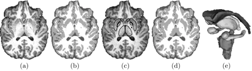
(a) (b) (c) (d) (e)
Fig. 2. Real 3T brain scan (a). (b): tissue segmentation by FBM-T. (c) and (d): struc-ture segmentation by FBM-TS and corresponding improved tissue segmentation. (e): 3-D reconstruction of the 17 segmented structures: the two lateral ventricules, cau-dates, accumbens, putamens, thalamus, pallidums, hippocampus, amygdalas and the brain stem. The computational time was < 15min after the registration step.
8 Draft Version of MICCAI’08 Paper
5
Discussion
The results obtained with our approach are very satisfying and compare favor-ably with other existing methods. The strength of our fully Bayesian joint model is to be based on the specification of a coherently linked system of conditional models for which we make full use of modern statistics to ensure tractability. The tissue and structure models are linked conditional MRF’s that capture several level of interactions. They incorporate 1) spatial dependencies between voxels for robustness to noise, 2) relationships between tissue and structure labels for co-operative aspects and 3) a priori anatomical information via the MRF external field parameters for consistency with expert knowledge. Besides, the addition of a conditional MRF model on the intensity distribution parameters allow to han-dle local estimations for robustness to nonuniformities. In this setting, the whole consistent treatment of MR brain scans is made possible using the framework of Generalized Alternating Minimization (GAM) procedures that generalize the standard EM framework. Another advantage of this approach is that it is made of steps that are easy to interpret and could be enriched with additional infor-mation. In particular, results currently highly depend on the atlas registration step which could be introduced in our framework as in [9]. Also a different kind of prior knowledge could be considered such as the fuzzy spatial relations used in [3]. Other on going work relates to the interpolation step we added to in-crease robustness to nonuniformities at a voxel level. We believe this stage could be generalized and incorporated in the model by considering successively vari-ous degrees of locality, mimicking a multiresolution approach and refining from coarse partitions of the entire volume to finer ones. Also considering more general weights w, to deal with possible conflicts between tissue and structure labels, is possible in our framework and would be an interesting refinement.
References
1. Shattuck, D., et al: Magnetic resonance image tissue classification using a partial volume model. NeuroImage 13(5) (2001) 856–876
2. Rajapakse, J.C., Giedd, J.N., Rapoport, J.L.: Statistical approach to segmentation of single-channel cerebral MR images. IEEE TMI 16(2) (1997) 176–186
3. Scherrer, B., Dojat, M., Forbes, F., Garbay, C.: LOCUS: LOcal Cooperative Unified Segmentation of MRI brain scans. In: MICCAI 2007, Brisbane, Australia
4. Byrne, W., Gunawardana, A.: Convergence theorems of Generalized Alternating Minimization Procedures. J. Machine Learning Research 6 (2005) 2049–2073 5. Kumar, S., Hebert, M.: Discriminative random fields. Int. J. Comput. Vision 68(2)
(2006) 179–201
6. Gelman, A., et al: Bayesian Data Analysis. Chapman & Hall, 2nd edition (2004) 7. Besag, J.: On the statistical analysis of dirty pictures. J. Roy. Statist. Soc. Ser. B
48(3) (1986) 259–302
8. Besag, J.: Spatial interaction and the statistical analysis of lattice systems. J. Roy. Statist. Soc. Ser. B 36(2) (1974) 192–236
9. Pohl, K.M., Fisher, J., Grimson, W.E.L., Kikinis, R., Wells, W.M.: A Bayesian model for joint segmentation and registration. NeuroImage 31(1) (2006) 228–239