The Airlift Planning Problem

The MIT Faculty has made this article openly available.

Please share

how this access benefits you. Your story matters.

Citation

Bertsimas, Dimitris et al. “The Airlift Planning Problem.”

Transportation Science, 53, 3 (May 2019): 623-916 © 2019 The

Author(s)

As Published

10.1287/TRSC.2018.0847

Publisher

Institute for Operations Research and the Management Sciences

(INFORMS)

Version

Author's final manuscript

Citable link

https://hdl.handle.net/1721.1/129699

Terms of Use

Creative Commons Attribution-Noncommercial-Share Alike

issn 0041-1655 | eissn 1526-5447 | 00 | 0000 | 0001 _{0000 INFORMSc}

The Airlift Planning Problem *

Sloan School of Management and Operations Research Center, Massachusetts Institute of Technology, 77 Massachusetts Avenue, Cambridge, MA, 02139; [email protected]

Allison Chang

Lincoln Laboratory, Massachusetts Institute of Technology; 244 Wood Street, Lexington, MA, 02420; [email protected] Velibor V. Miˇsi´c

Anderson School of Management, University of California, Los Angeles, 110 Westwood Plaza, Los Angeles, CA, 90095; [email protected]

Nishanth Mundru

Operations Research Center, Massachusetts Institute of Technology, 77 Massachusetts Avenue, Cambridge, MA, 02139; [email protected]

The United States Transportation Command (USTRANSCOM) is responsible for planning and executing the transportation of United States military personnel and cargo by air, land and sea. The airlift planning problem faced by the air component of USTRANSCOM is to decide how requirements (passengers and cargo) will be assigned to the available aircraft fleet and the sequence of pickups and dropoffs that each aircraft will perform in order to ensure that the requirements are delivered with minimal delay and with maximum utilization of the available aircraft. This problem is of significant interest to USTRANSCOM due to the highly time-sensitive nature of the requirements that are typically designated for delivery by airlift, as well as the very high cost of airlift operations. At the same time, the airlift planning problem is extremely difficult to solve due to the combinatorial nature of the problem and the numerous constraints present in the problem (such as weight restrictions and crew rest requirements). In this paper, we propose an approach for solving the airlift planning problem faced by USTRANSCOM based on modern, large-scale optimization. Our approach relies on solving a large-scale mixed-integer programming model that disentangles the assignment decision (which aircraft will pickup and deliver which requirement) from the sequencing decision (in what order the aircraft will pickup and deliver its assigned requirements), using a combination of heuristics and column generation. Through computational experiments with both a simulated data set and a planning data set provided by USTRANSCOM, we show that our approach leads to high-quality solutions for realistic instances (e.g., 100 aircraft and 100 requirements) within operationally feasible time frames. Compared to a baseline approach that emulates current practice at USTRANSCOM, our approach leads to reductions in total delay and aircraft time of 8 to 12% in simulated data instances and 16 to 40% in USTRANSCOM’s planning instances.

Key words : pickup and delivery with time windows; mixed-integer programming; column generation; local search; construction heuristics

1.

Introduction

The United States Transportation Command (USTRANSCOM) is the main entity responsible for the transportation of personnel and cargo for the United States military across the globe. Of the three modes of transportation employed by USTRANSCOM – air, land and sea – transportation by air is often the most efficient means of delivering requirements (passengers and cargo) and thus is often the mode of choice for many high-priority and short-notice missions.

The planning of airlift missions is of critical importance to USTRANSCOM, for two reasons. First, due to the time-sensitive nature of requirements transported by air, a primary concern for

*This material is based upon work supported under Air Force Contract No. FA8721-05-C-0002. Any opinions, findings, conclusions or recommen-dations expressed in this material are those of the author(s) and do not necessarily reflect the views of the U.S. Air Force.

USTRANSCOM is that requirements be picked up and delivered within their predefined time windows with minimal or no delay. Second, transporting requirements by air is expensive: a recent RAND study estimates that airlift missions cost between $9,000 and $12,000 per flying hour for certain aircraft types (Robbert 2013). By carefully planning its airlift missions, USTRANSCOM could potentially ensure that all requirements are delivered on time, while doing so with a more efficient use of its aircraft – more precisely, using fewer aircraft and through shorter missions.

At the same time, planning efficient airlift missions is difficult. The primary reason for this is the combinatorial nature of the problem: planners must decide which requirements will be picked up and delivered by which aircraft, and in what sequence those aircraft will pick up and deliver those requirements. This naturally leads to an extremely large number of possible schedules. A secondary reason is that airlift missions are governed by a multitude of constraints: requirements must be picked up and delivered within their defined time windows; the total weight of the requirements being transported by each aircraft at any time cannot exceed the weight capacity of that aircraft; and the schedule must respect aircraft crew rest constraints. At present, planners schedule each requirement one at a time, and look for opportunities to combine some missions with others to reduce transportation costs. However, this process is largely manual and ad hoc, and there is a need for a decision support infrastructure to systematically design schedules that deliver requirements with minimal delay and with maximum utilization of the available aircraft.

In this paper, we present a methodology for designing airlift schedules for USTRANSCOM based on modern, large-scale optimization. This method is based on solving a large-scale mixed-integer programming (MIP) model of the problem using a combination of heuristics – an initialization heuristic and a local search heuristic – and column/constraint generation. This method is capable of efficiently producing high-quality schedules – that is, ones that deliver requirements on time or with minimal delay, with a minimal amount of aircraft hours.

We make the following contributions:

1. We propose an MIP formulation of the airlift planning problem. This formulation jointly decides the assignment of requirements to aircraft and the sequence of pickups and dropoffs so as to minimize a weighted combination of delay and uptime (the total aircraft-hours required by the schedule). Our formulation has a number of features not typically found in prior models for pickup and delivery problems, such as the ability of aircraft to rest, constraints on rest periods and active times, and time windows that are both hard and soft; we show how to model these various features using the language of MIP.

2. Motivated by the difficulty of the original MIP problem, we propose a reformulation of the problem as a large-scale MIP, where the decision variables correspond to assigning a set of require-ments and the sequencing of each aircraft’s mission is captured through the objective function coefficients. This reformulation allows us to decouple the decision of which requirements will be assigned to which aircraft from the decision of how to sequence the pickup and dropoff events of each aircraft. We propose a three-phase method for solving this reformulated problem: in the first phase, we run an initialization heuristic that constructs an initial feasible assignment of require-ments to aircraft; in the second phase, we improve this assignment using a local search heuristic; and in the final phase, we use column generation to further improve the solution and to also obtain a lower bound on the quality of the ultimate solution. Unlike most prior approaches to pickup and delivery problems, our three-phase method makes use of a smaller version of our original MIP prob-lem for sequencing each aircraft; this is advantageous, because each aircraft is sequenced optimally, but also necessary in order to respect the operational constraints required by USTRANSCOM.

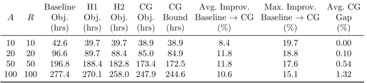
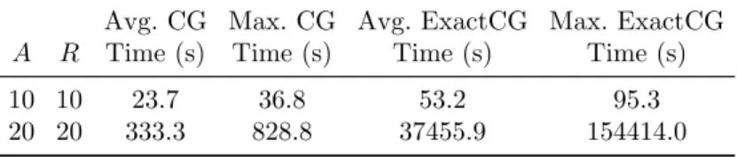
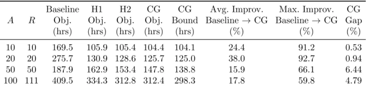
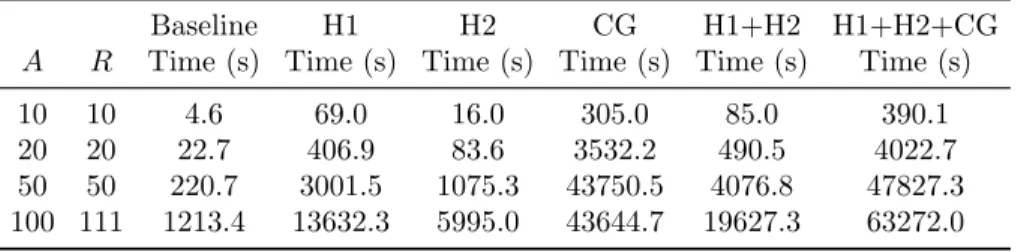
3. We demonstrate the value of this method through computational experiments with both a simulated data set and a planning data set provided to us by USTRANSCOM. Using our two heuristics, we are able to obtain high quality solutions for large instances (100 aircraft and 100 requirements) within six hours; the column generation algorithm we propose further improves these solutions and provides an approximation of the suboptimality gap, which is below 1.5% on average for the simulated data instances, and 7% on average for the USTRANSCOM planning

instances. More importantly, the solutions produced by our method significantly outperform a baseline approach that emulates current practice at USTRANSCOM; in comparison, our overall method leads to average reductions in total delay and uptime of 8 to 12% in the simulated data instances and 16 to 40% in USTRANSCOM’s internal planning instances.

The rest of the paper is organized as follows. In Section 2, we present a survey of related work. In Section 3, we define the problem and provide an initial MIP formulation of the problem. In Section 4, we present a large-scale optimization approach for efficiently solving the problem defined in Section 3. We present the results of our computational study in Section 5. Finally, in Section 6, we conclude.

2.

Literature review

We divide our review of the literature in two parts. We first survey the large body of work on vehicle routing problems, which are closely related to the airlift planning problem. We then survey related work in other areas, specifically in air traffic management and dynamic resource allocation. Vehicle routing. The airlift planning problem falls in the general category of pickup and delivery problems with time windows (PDPTW). The PDPTW is a generalization of the vehicle routing problem, and consequently is also an NP-hard problem (Garey and Johnson 1979). The vehicle routing problem involves designing a set of routes, originating and terminating at a single depot, for a fleet of vehicles that service a set of customers with known demands, with each customer being serviced exactly once. For a general survey of vehicle routing problems, we direct the reader to Laporte (2007) and Toth and Vigo (2014).

PDPTW involves designing a set of minimum-cost routes to satisfy transportation requests (requirements). Each requirement has a pickup and dropoff location, and a corresponding size. The decision maker has a fleet of vehicles, each with some capacity and predefined start and end locations. Each requirement has to be transported by one vehicle from its pickup location (origin) to its dropoff location (destination). The routes must satisfy the precedence relations of pickup and delivery points, along with the time windows imposed by them. For a comprehensive review of the PDPTW literature, we refer the reader to Desrochers et al. (1988), Savelsbergh and Sol (1995), Cordeau et al. (2004) and Toth and Vigo (2014, Chap. 6 and 7). In the PDPTW, all vehicles depart from and return to a central depot. The airlift planning problem is best described as a PDPTW with multiple depots, along with other real life constraints/features such as maximum active time (the aircraft cannot operate beyond a certain amount of time without initiating a rest period) and minimum rest time (when the aircraft rests, it must rest for at least some minimum number of hours). In addition, the time constraints in our problem have both a “hard” component (each requirement must be picked up/dropped off within some time window) and a “soft” component (if a requirement is picked up/dropped off past a certain time within that time window, it is considered late, and the objective penalizes this lateness).

Many heuristics have been proposed for the PDPTW problem, such as tabu search (Nanry and Barnes 2000), simulated annealing (Bent and Van Hentenryck 2006) and large neighborhood search (Ropke and Pisinger 2006). Within this body of work, there exist some approaches that are similar to our initialization and local search heuristics (Algorithms 3 and 4 in Section 4.4 respectively). For example, in Nanry and Barnes (2000), the initial feasible solution is produced by an insertion algorithm that attempts to insert a pickup-delivery pair onto the first vehicle and if more than one feasible insertion point exists, then the procedure picks the insertion that least increases the partial solution’s travel time; if no feasible insertion point exists, then a new vehicle is added to the solution. This procedure resembles our initialization heuristic, which also builds a partial assignment of requirements to aircraft and seeks to assign a requirement in a way that least increases the total objective of the partial solution, while maintaining feasibility. Nanry and Barnes (2000) also discuss a type of neighborhood used in their tabu search which involves removing a pickup-delivery pair from its current vehicle route and inserting it into one of

the other vehicle routes; this procedure resembles our local search heuristic, which also involves moving one requirement from its current aircraft and assigning it to a different aircraft. One major difference between the heuristics we consider from those considered before is that in most previously considered heuristics, the insertion of a pickup-delivery pair into a vehicle route leaves the order of the other pickup-delivery pairs intact; stated differently, one does not re-optimize the sequence of pickup-delivery pairs after each insertion. In contrast, our heuristics (Algorithm 3 and 4) involve exactly re-optimizing each aircraft’s sequence whenever the set of requirements assigned to that aircraft is changed (when a requirement is added to the aircraft, or a requirement is removed from the aircraft). This is advantageous because it does not leave value on the table, so to speak, with regard to the sequence of each aircraft; each aircraft’s sequence achieves the lowest possible objective value. From an implementation point of view, inserting a pickup and a dropoff into an existing event sequence in the airlift planning problem is also not straightforward to do due to the constraints on weight and active time, and also due to the fact that aircraft may choose to rest for a variable time period between events.

Outside of heuristic methods, a number of previous studies have considered the use of column generation methods and branch-and-price methods for solving the PDPTW exactly. Column gen-eration was first applied to PDPTW by Dumas, Desrosiers, and Soumis (1991); they formulated the problem as a set partitioning problem, where each column maps to a feasible vehicle route and each constraint corresponds to a request that must be satisfied exactly once, and they solved the pricing subproblem using dynamic programming and label elimination methods. Savelsbergh and Sol (1998) later proposed a branch-and-price method for solving the problem, where the pricing subproblem is solved using a combination of construction and improvement heuristics. Ropke and Cordeau (2009) propose a branch-cut-price approach. In their approach, the pricing subproblem is formulated as a constrained shortest path problem; when it needs to be solved exactly, it is solved using labeling algorithms, and otherwise it is solved using a combination of large neighborhood search, label heuristics and heuristics based on construction and improvement. Other examples of column generation approaches for PDPTW include Xu et al. (2003) and Sigurd, Pisinger, and Sig (2004).

The column generation approach that we consider in this paper is similar to these previously proposed approaches; the master problem that we solve is effectively a set partitioning problem, where the variables correspond to whether an aircraft a is assigned to a set of requirements S and we must iteratively add (a, S) pairs using column generation. However, our approach differs in several ways. First, we use column generation for the purpose of improving the solution obtained by our heuristics and for obtaining a lower bound on the quality of that solution; we do not embed our column generation within a branch-and-price scheme in order to solve the problem exactly. Second, like some prior applications of column generation to PDPTW, we also use a heuristic approach for solving the pricing subproblem, but our approach differs in that it is a set-based local search. More precisely, we perform a local search over sets of requirements S that lead to the lowest reduced cost, where for each set S we solve a single-aircraft sequencing problem in order to compute the reduced cost (cf. our comparison of our heuristic algorithms); in other words, our subproblem heuristic exactly re-optimizes the actual sequence of pickups and dropoffs for each set of requirements (i.e., the heuristic does not additionally involve a local search over the sequence of pickups and dropoffs). We are not aware of a similar approach in the vehicle routing literature. Outside of the vehicle routing literature, a similar algorithm was proposed in the operations management literature, in the context of finding an assortment (set of products) that maximizes a black-box revenue function and was shown to perform well for a variety of revenue functions (Jagabathula 2014).

Some papers have also considered mixed-integer programming approaches not based on set partitioning and column generation. Ropke, Cordeau, and Laporte (2007) consider a branch-and-cut approach for solving a “two-index” formulation of the PDPTW, where the binary decision variables indicate whether a given pickup/delivery is performed immediately before a different pickup/delivery. Lu and Dessouky (2004) solve the multiple vehicle pickup and delivery problem

using branch-and-cut. Mahmoudi and Zhou (2016) consider the PDPTW with many vehicles and propose a multi-commodity flow formulation of it using a state-space-time network representa-tion; they consider a Lagrangian relaxation of the multi-commodity flow problem, which leads to a collection of single vehicle routing subproblems that can be solved using a forward dynamic programming algorithm.

Some work in PDPTW has focused on air transportation. One recent example is the paper of Carnes et al. (2013), which considers the assignment and sequencing of aircraft for performing non-emergency transportation of patients between different facilities. The problem has some similarities to the one that we consider. For example, each patient is analogous to a requirement in our context, and each aircraft is limited in how many requests (requirements/patients) that it can carry at any time. However, some constraints are different and do not have analogs in our problem – for example, a schedule in Carnes et al. (2013) cannot transport infectious patients with uninfected patients, and must spend additional time on the ground after delivering an infectious patient to be disinfected. Similarly, there is no constraint in Carnes et al. (2013) analogous to our rest and maximum active time constraints. In addition, the solution methods are different. In Carnes et al. (2013), the problem is solved through a set partitioning formulation, but because of the scale of their problem and constraints on how many requests can be assigned to each aircraft, the columns of the formulation can be completely enumerated and their costs precomputed, which allows them to solve the problem directly to full optimality. In contrast, this is not possible in our setting, because of the scale and the lack of a similar constraint on how many requirements can be assigned to a single aircraft; as a result, we must turn to both column generation and initialization/local search heuristics.

We summarize the key differences between our paper and the existing PDPTW literature as follows:

1. Problem setting. Our problem contains many elements not typically found in PDPTW problems, such as hard and soft time windows, variable wait times, constraints on maximum active time, and combined delay and uptime as an objective. To the best of our knowledge, no other paper has studied a PDPTW problem with this specific combination of features, at the scale required by USTRANSCOM.

2. Heuristics. Both our initialization and local search heuristics involve modifying an assign-ment of requireassign-ments to aircraft, where the value of an assignassign-ment is obtained by solving a small, single aircraft MIP problem for each aircraft to sequence the pickups and dropoffs; in this way, the single aircraft MIP problem is used as a black box. This contrasts with many other construction and local search heuristics for PDPTW that do not use MIP, but directly remove pickup/dropoff events from one vehicle’s sequence and insert them into the sequence of a different vehicle. Our use of the single aircraft MIP is necessary for our problem setting because, as mentioned earlier, it is not straightforward to insert events into a sequence in a way that respects the various constraints of the problem.

3. Column generation. Our column generation approach differs in two ways from existing column generation approaches. First, our master problem is not a pure set partitioning problem, as is often the case in many PDPTW problems, but also involves an assignment decision; this difference is important because the aircraft are heterogeneous in their travel times, capacities and the ports at which they must start and end their missions. Second, the subproblem in our column generation algorithm is solved heuristically, again using the aforementioned single aircraft MIP problem as a black box. As with our initialization and local search heuristics, the use of the single aircraft MIP problem is a practical necessity in order to ensure feasibility with respect to all of the constraints of the problem; the features of our problem complicate the use of traditional methods such as dynamic programming. Third, we use column generation in a heuristic manner, to improve the solution obtained from our local search heuristic, as opposed to using it within a branch-and-price method. As such, our column generation method can be implemented with less effort and requires less time to run than branch-and-price. However, unlike branch-and-price,

the final integer solution produced by our column generation algorithm is not guaranteed to be optimal.

Other areas. Outside of vehicle routing, the present paper is related to some other work in air traffic management and dynamic resource allocation.

The air traffic flow management (ATFM) problem is to decide what flow management actions to take for a set of flights – such as ground holding, airborne holding and rerouting – so as to minimize the aggregate delay of those flights, while respecting constraints on the capacity of each sector of airspace. We focus on some specific examples of work in this area; for a more detailed review of this literature, the reader is referred to Vossen, Hoffman, and Mukherjee (2012). Bertsimas and Stock Patterson (1998) propose an integer programming formulation of the problem where the only allowed interventions are ground holding and speed control, and each aircraft’s path is fixed. Bertsimas and Stock Patterson (2000) extended this approach to allow for re-routing decisions by considering a dynamic, multi-commodity flow problem, which they solve using a combination of Lagrangian relaxation, randomized rounding and solving an integer packing problem. Bertsimas, Lulli, and Odoni (2011) build on both of these previous papers by proposing an integer program-ming model that allows for the full range of flow management actions and that can be solved directly using commercial software for very large-scale instances (for example, the continental United States network).

There are similarities and differences between the airlift planning problem and the ATFM prob-lem studied in the above papers. Our probprob-lem bears some resemblance to the ATFM probprob-lem in that routing decisions are somewhat similar to the scheduling decisions (what sequence should an aircraft perform its assigned pickups and dropoffs) in the airlift planning problem; unlike the ATFM problem, though, the airlift planning problem additionally involves an assignment decision, which the ATFM problem does not. Another point of difference has to do with whether the air-craft are coupled or not. Although one can consider constraints that couple airair-craft together in our problem (such as so-called “maximum-on-ground” constraints, which limit how many aircraft can be present at an airbase at any moment in time), we do not consider such constraints in this paper, and so the aircraft in our model are decoupled. In contrast, the sector capacity constraints in the ATFM problem (i.e., there can be no more than five aircraft in a sector) effectively cou-ple the aircraft together, and one cannot plan the flight path/flow management decisions for one aircraft independently of another. From a modeling perspective, our approach for the airlift plan-ning problem involves an integer programming model where the time of each pickup/dropoff is represented through continuous variables, and the sequence of events is represented through slot-based variables (i.e., event e is the pth event in aircraft a’s event sequence). In contrast, time is discretized in Bertsimas and Stock Patterson (1998, 2000) and Bertsimas, Lulli, and Odoni (2011), and the sequence is represented through “by” variables (i.e., flight f reaches sector j by time t). Furthermore, from a solution perspective, our approach decouples the assignment and schedul-ing decisions and solves the problem usschedul-ing heuristics and column generation; in Bertsimas and Stock Patterson (1998, 2000) and Bertsimas, Lulli, and Odoni (2011), one directly solves the full integer programming formulation of the problem.

Beyond the ATFM problem, our work is related to the more general problem of dynamic resource allocation, where one must allocate requests to resources so as to complete them within some predefined time windows with minimum cost. One salient example in this area is Bertsimas, Gupta, and Lulli (2014), who propose a general integer programming formulation for dynamic resource allocation and a specialized algorithm for solving it based on adjustable time windows, with the ATFM problem as an application of the framework. The formulation in Bertsimas, Gupta, and Lulli (2014) is similar to those in Bertsimas and Stock Patterson (1998, 2000) and Bertsimas, Lulli, and Odoni (2011), in that the main decision variables model whether a request has begun utilizing a resource by some discrete time; as mentioned in the discussion above, this formulation differs significantly from our slot-based formulation.

3.

Problem definition

In this section, we define the airlift planning problem. We begin by describing the notation for the parameters and decision variables in Section 3.1. Then, in Section 3.2, we provide a mixed-integer programming (MIP) formulation of the problem, and describe in detail the objective function and the constraints of the formulation.

3.1. Notation

We assume that there are R requirements that must be transported, indexed from 1 to R, and we let R = {1, . . . , R} denote the set of requirements. We assume that there are A aircraft that can be used to transport the requirements, indexed from 1 to A and let A = {1, . . . , A} denote the set of aircraft. We will model the problem by defining four primitive events that may occur over the planning horizon:

1. Pickup(r): requirement r is picked up. 2. Dropoff(r): requirement r is dropped off. 3. Start(a): aircraft a begins its mission. 4. End(a): aircraft a ends its mission.

We use E to denote the set of all possible events:

E = {Pickup(r) r ∈ R} ∪ {Dropoff(r) r ∈ R} ∪ {Start(a) a ∈ A} ∪ {End(a) a ∈ A}. Each event may only be performed by one aircraft. All Pickup(r) and Dropoff(r) events must be executed, and may be executed by any aircraft. We assume that the same aircraft used to execute Pickup(r) must also be used to execute Dropoff(r). The Start(a) and End(a) events must be executed by aircraft a if and only if aircraft a is used in the schedule.

Each event e must occur at a specific location or “port”. We let τe,e0,a denote the travel time

of aircraft a from the port of event e to the port of event e0_{. We let `}

e denote the earliest time

by which event e may be executed, ue denote the latest time by which event e may be executed

without penalty, and Be denote the maximum slack of event e, that is, Be is the largest amount of

time by which event e may be executed past ue. Stated differently, an event may be executed at any

time t within [`e, ue+ Be]; if t is within [`e, ue], there is no penalty, but if t is within (ue, ue+ Be],

the requirement is deemed late, where the delay/slack is given by t − ue. The event e cannot be

executed past ue+ Be or before `e.

We use T to denote the end of the time horizon, which is the maximum of all of the times by which any event may be executed; mathematically, it is defined as

T = max

e∈E (ue+ Be).

Similarly, we assume that the problem starts at time 0; the interval [0, T ] thus defines the planning horizon of the problem.

We let wedenote the change in an aircraft’s weight associated with executing event e. For Start(a)

and End(a) events, we= 0; for Pickup(r) events, wPickup(r)> 0 (performing a pickup leads to an

increase in the carried weight of the aircraft), and for Dropoff(r) events, wDropoff(r)= −wPickup(r)< 0

(performing a dropoff leads to a decrease in the carried weight of the aircraft). For each aircraft a ∈ A, we use Wa to denote the weight capacity of that aircraft; at any point in time, the total

weight carried by aircraft a cannot exceed Wa. We assume that for each requirement r, the weight

of that requirement fits within the capacity of at least one of the aircraft (i.e., for each r, there exists an a ∈ A such that wPickup(r)≤ Wa).

Each aircraft is subject to rest constraints. We let γadenote the maximum active time of aircraft

a, where the active time is defined as the accumulated time that the aircraft has been in the air since its last rest period. We let δa denote the minimum rest time of aircraft a; this is the least

amount of time that an aircraft must rest on the ground before it can return to flying and executing its remaining events.

The objective that we will optimize consists of a weighted combination of the total delay/slack of all events plus the total uptime of all aircraft used in the schedule, where the uptime of aircraft a is defined as the time from the Start(a) event to the End(a) event of aircraft a. We use πe to

denote the priority of event e; the priority of an event is the weight coefficient of that event in the objective. We use C to denote the objective weight coefficient of the total uptime of all of the aircraft; we assume that C > 0.

3.2. Formulation

In this section, we define the airlift planning problem by formulating it as a mixed-integer pro-gramming (MIP) problem.

We begin by modeling each aircraft as having a sequence of P slots. Each slot fits at most one event. Since any one aircraft can perform at most 2R + 2 events – the Pickup(r) and Dropoff(r) event for each requirement in R, as well as the Start(a) and End(a) events of that aircraft – we set the number of slots P to be 2R + 2. In addition, for the purpose of defining the MIP formulation, let us also define E (R) to be the set of pickup and dropoff events for all requirements:

E(R) = {Pickup(r) r ∈ R} ∪ {Dropoff(r) r ∈ R}.

Additionally, let us define E (a, R) as the set of pickup and dropoff events for all requirements in R, together with the start and end events for aircraft a, formally,

E(a, R) = {Pickup(r) r ∈ R} ∪ {Dropoff(r) r ∈ R} ∪ {Start(a), End(a)}.

We define our decision variables as follows. We let xe,a,p be a binary variable that is 1 if aircraft

a executes event e in its pth slot, and 0 otherwise. We let ye,e0_,a,p be a binary variable that is 1 if

aircraft a executes event e in slot p of its sequence and event e0 in slot p + 1 of its sequence, and 0 otherwise. We let za,p be a binary variable that is 1 if aircraft a rests immediately after executing

the event in slot p. We let ta,p be a continuous variable that represents the time at which aircraft a

executes the event in slot p. We let se,a,p be a continuous variable that represents the delay/slack

of event e if it is performed by aircraft a in slot p of that aircraft’s sequence. Finally, we use ωa,p

to denote the accumulated active time from aircraft a’s Start(a) event to immediately before the event in slot p of aircraft a’s sequence.

minimize x,y,z,t,s,ω X e∈E πe X a∈A P X p=1 se,a,p+ C X a∈A

(ta,P− ta,1) (1a)

subject to X a∈A P X p=1 xe,a,p= 1, ∀ e ∈ E(R), (1b) P X p=1 xStart(a),a,p≤ 1, ∀ a ∈ A, (1c) P X p=1 xEnd(a),a,p= xStart(a),a,1, ∀ a ∈ A, (1d) X e∈E(a,R)

xe,a,p≤ xStart(a),a,1, ∀ a ∈ A, p ∈ {1, . . . , P }, (1e)

X e∈E(a,R) xe,a,p0≤ 1 − x_End(a),a,p, ∀ a ∈ A, p ∈ {2, . . . , P − 1}, p0∈ {p + 1, . . . , P }, (1f) X e∈E(a,R) xe,a,p+1≤ X e∈E(a,R) xe,a,p, ∀ a ∈ A, p ∈ {1, . . . , P − 1}, (1g)

P X p=1 xDropoff(r),a,p= P X p=1 xPickup(r),a,p, ∀ r ∈ R, a ∈ A, (1h) p X p0=1 xPickup(r),a,p0≥ p X p0=1 xDropoff(r),a,p0, ∀ r ∈ R, a ∈ A, p ∈ {1, . . . , P }, (1i)

ye,e0,a,p≥ xe,a,p+ xe0,a,p+1− 1,

∀ a ∈ A, e, e0_{∈ E(a, R), p ∈ {1, . . . , P − 1}, (1j)}

ye,e0_,a,p≤ x_e,a,p, ∀ a ∈ A, e, e0∈ E(a, R), p ∈ {1, . . . , P − 1}, (1k)

ye,e0_,a,p≤ x_e0_,a,p+1, ∀ a ∈ A, e, e0∈ E(a, R), p ∈ {1, . . . , P − 1}, (1l)

X e∈E(a,R) p X p0₌₁ wexe,a,p0≤ Wa, ∀ a ∈ A, e ∈ E(a, R), p ∈ {1, . . . , P }, (1m) ta,p+1≥ ta,p+ X e,e0_∈E(a,R)

τe,e0_,ay_e,e0_,a+ δ_az_a,p,

∀ a ∈ A, p ∈ {1, . . . , P − 1}, (1n) ta,p≥ X e∈E(a,R) `exe,a,p, ∀ a ∈ A, p ∈ {1, . . . , P }, (1o) ta,p≤ X e∈E(a,R) (uexe,a,p+ se,a,p) + T  1 − X e∈E(a,R) xe,a,p  , ∀ a ∈ A, p ∈ {1, . . . , P }, (1p)

se,a,p≤ Be· xe,a,p, ∀ a ∈ A, e ∈ E(a, R), p ∈ {1, . . . , P }, (1q)

ωa,1= 0, ∀ a ∈ A, (1r)

ωa,p= ωa,p−1+

X

e,e0∈E(a,R)

τe,e0,a· ye,e0,a,p−1, ∀ a ∈ A, p ∈ {2, . . . , P }, (1s)

ωa,q0− ω_a,q≤ γ_a·  1 + q0−1 X p=q za,p  , ∀ a ∈ A, q ∈ {1, . . . , P − 1}, q0_{∈ {q + 1, . . . , P }, (1t)}

xe,a,p∈ {0, 1}, ∀ a ∈ A, e ∈ E(a, R), p ∈ {1, . . . , P }, (1u)

za,p∈ {0, 1}, ∀ a ∈ A, p ∈ {1, . . . , P }, (1v)

ye,e0_,a,p≥ 0, ∀ e, e0∈ E(a, R), a ∈ A, p ∈ {1, . . . , P − 1}, (1w)

ta,p, ωa,p≥ 0, ∀ a ∈ A, p ∈ {1, . . . , P }, (1x)

se,a,p≥ 0, ∀ e ∈ E(a, R), a ∈ A, p ∈ {1, . . . , P }. (1y)

To understand the formulation, let us first describe each relevant group of constraints, followed by the objective function.

Mission constraints: Constraint (1b) requires that each pickup and dropoff event happens; each such event must be assigned to the slot of some aircraft. Constraint (1c) ensures that the Start(a) event of each aircraft a is executed at most once by aircraft a. Constraint (1d) ensures that aircraft a executes the End(a) event if and only if it executes the Start(a) event in slot 1. Constraint (1e) ensures that in each slot of each aircraft, there can be at most one event if the aircraft executes Start(a) in slot 1, and there is no event if that aircraft does not start in slot 1. Constraints (1e)

and (1c) together ensure that an aircraft performs any events if and only if it executes Start(a) in slot 1; in other words, Start(a) is always the event of the first slot of aircraft a if aircraft a is to be used in the solution. Constraint (1f) ensures that there are no events in the slots of aircraft a after the End(a) event (if the aircraft ends its mission, it cannot continue performing pickups and dropoffs). Constraint (1g) requires that if there is an event in slot p + 1, there must be an event in slot p; stated differently, there cannot be any empty slots between Start(a) and End(a).

Pickup/dropoff constraints: Constraint (1h) ensures that a requirement must be picked up and dropped off by the same aircraft. Constraint (1i) ensures that, in terms of slots, Pickup(r) always comes before Dropoff(r). (The left hand side of the constraint is 1 if Pickup(r) happens by slot p and 0 otherwise, and the right hand side is 1 if Dropoff(r) happens by slot p and 0 otherwise; the constraint requires that if a requirement is dropped off by slot p, it must have been picked up by slot p as well.)

Transition constraints: Constraints (1j) through (1l) are forcing constraints that ensure that the y variables take their correct values based on the x variables.

Capacity constraint: Constraint (1m) requires that the weight carried by aircraft a at any slot p cannot exceed the capacity Wa of that aircraft.

Travel time dynamics constraint: Constraint (1n) ensures that the ta,p variables respect travel

times. More precisely, this constraint requires that the event in slot p + 1 of aircraft a can be performed no earlier than the time of slot p of aircraft a plus the correct travel time (encoded by the weighted sum of ye,e0,a,p variables) and the minimum rest time δa if the aircraft rests after

performing the event of slot p.

Time window constraints: Constraint (1o) ensures that the time at which aircraft a performs whatever event is in slot p satisfies the earliest allowable time `e of that event. Constraint (1p)

ensures that the time at which aircraft a performs the event in slot p satisfies the latest allowable time ue, adjusted by the slack/delay se,a,p of that event. In the case that there is no event assigned

to slot p of aircraft a, these constraints become vacuous; the right-hand side of constraint (1o) becomes 0, while the right-hand side of constraint (1p) becomes T . Constraint (1q) requires that the slack/delay variable se,a,p is bounded by Be if event e happens in slot p of aircraft a and is

forced to zero otherwise.

Active time constraints: Constraints (1r) and (1s) model the dynamics of the accumulated active time from the start of the aircraft’s mission. Constraint (1t) ensures that the active time accumulated between any two periods does not exceed how much active time is afforded by the rests taken over those two periods.

Variable definitions: Finally, constraints (1u) through (1y) define the variables. Note that since the x variables are binary, the forcing constraints (1j) through (1l) ensure that the y variables are automatically forced to their correct binary values; thus, we can model the y variables as continuous variables.

Objective function: The objective (1a) consists of two parts: the first part represents the priority-weighted sum of slacks/delays, while the second part represents the priority-weighted total uptime of all of the aircraft.

Note that since C > 0, ta,P− ta,1 will always correctly reflect the uptime of aircraft a. If aircraft

a is not used, all y variables corresponding to aircraft a will be zero, and ta,1, . . . , ta,P are free to

weight C, we will have at optimality that ta,1= · · · = ta,P, so that ta,P − ta,1 will thus be zero.

In the case that aircraft a is used, let p0 _{be the slot at which End(a) occurs; then, for every slot}

p ≥ p0_{, all of the y variables corresponding to those slots are zero, and the variables t}

a,p0+1, . . . ta,P

are free to take any value between ta,p0 and T . Since C is positive, we will have at optimality that

ta,p0= ta,p0+1= · · · = ta,P; moreover, if aircraft a is used, then the event in slot 1 must be Start(a).

Thus, ta,P− ta,1 again correctly captures the uptime.

We remark that problem (1) above is formulated in terms of slots. One may wonder if the problem can be formulated more compactly, by using a formulation that models whether event i precedes event j (see, for example, Desrochers et al. 1988, p. 69). In order to model event times correctly in such a framework, one must use big-M constraints, which generally leads to weaker MIP formulations. Furthermore, our experimentation with this type of modeling approach in both the full aircraft problem as well as the single aircraft problem (problem (1) restricted to a single aircraft; see problem (2) in Section 4.1) did not yield an appreciable change in solution times.

4.

Method

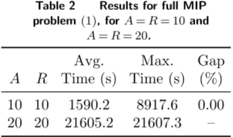
As stated in Section 3, the formulation of the problem (problem (1)) in Section 3 is for the purpose of clearly defining the problem, as opposed to providing a path towards solving the problem. It turns out that problem (1) is too difficult to solve directly as a MIP; as we will see in Section 5.2, for small problems (A = R = 10), the problem can take as much as two hours to solve, and for slightly larger problems (A = R = 20), even the relaxation cannot be solved within a reasonable time frame.

Due to the difficulty of solving problem (1), we now focus our attention on an alternate approach for attacking the problem. This alternate approach is motivated by the fact that the problem consists of two coupled problems: we first must assign the requirements to the aircraft, and then we must sequence the events that each aircraft must perform. Solving both problems simultaneously within one formulation is very difficult, as acknowledged above. However, if one fixes an assignment of requirements to the aircraft, then the optimization problem simplifies considerably, for two reasons; each aircraft can be scheduled independently, leading to A independent optimization problems, and each optimization problem is a simpler one than the overall problem, since one major dimension of the problem – the assignment of requirements to aircraft – is eliminated.

In this section, we begin in Section 4.1 by describing a formulation for the single aircraft problem, where the set of requirements assigned to one aircraft is fixed, and one only has to sequence the events for that aircraft. Having defined the single aircraft problem, in Section 4.2 we describe an alternate, large-scale MIP reformulation of the full problem (1) from Section 3 that takes advantage of the coupled nature of the problem described above and the single aircraft problem defined in Section 4.1. We then develop in Section 4.3 a column generation approach for provably solving the LP relaxation of this problem. In Section 4.4, we additionally develop two heuristics – an initialization heuristic for finding an initial solution that is feasible and a local search heuristic for improving this initial solution – that can be used to warm start the column generation approach. Finally, in Section 4.5, we summarize the overall algorithmic approach.

4.1. Continuous-time MIP for single aircraft scheduling

We begin by describing our large-scale approach by defining the so-called single aircraft schedul-ing problem, which is the foundation for our overall algorithmic approach. In the sschedul-ingle aircraft scheduling problem, a set of requirements is assigned to one aircraft, and we wish to schedule the pickup and dropoff events for that aircraft in a way that minimizes the objective from problem (1) (the weighted combination of delay and uptime) restricted to that one aircraft.

Let a be the aircraft of interest, and let S ⊆ R be the set of requirements that is to be scheduled. We define the notation for this problem below, which is similar to the notation of the full problem (1), except without the need for the aircraft indices in the variables and constraints

since there is only a single aircraft involved.

Parameters. In addition to those parameters defined earlier in Section 3.1, we define some addi-tional parameters. We let E (a, S) denote the set of events that must be performed by aircraft a when it is assigned the set of requirements S; formally, it is defined as:

E(a, S) = {Start(a), End(a)} ∪ {Pickup(r) : r ∈ S} ∪ {Dropoff(r) : r ∈ S}.

Similarly to Section 3.2, we let P denote the number of slots in the formulation, which is the size of E (a, S); this is then simply P = 2|S| + 2.

Variables. The decision variables are defined as follows. For each event e ∈ E (a, S) and slot p ∈ {1, . . . , P } we let xe,p be a binary decision variable that is 1 if event e is performed in slot p, and 0

otherwise; we also let xby

e,p be a binary decision variable that is 1 if event e is performed by slot p.

For each e and p ∈ {1, . . . , P − 1}, we let ye,e0_,p be a binary decision variable that is 1 if event e is

performed in slot p, and event e0 _{is performed in slot p + 1. For each slot p, we let z}

p be a binary

decision variable that is 1 if the aircraft rests after performing the event of slot p, and 0 otherwise. We let tp be the time at which the aircraft starts to execute the event in slot p. We let se,p denote

the slack of event e if it is assigned to slot p. Finally, we let ωp denote the accumulated active time

of the aircraft at the start of slot p from the beginning of the aircraft’s mission. With these definitions, we now define the single aircraft scheduling problem.

minimize x,y,z,t,s,ω X e∈E(a,S) P X p=1 πese,p+ C(tP− t1) (2a) subject to P X p=1 xe,p= 1, ∀ e ∈ E(a, S), (2b) X e∈E(a,S) xe,p= 1, ∀ p ∈ {1, . . . , P }, (2c) xStart(a),1= 1, (2d) xEnd(a),P = 1, (2e) xe,1= x by e,1, ∀ e ∈ E(a, S), (2f) xe,p= xbye,p− x by e,p−1, ∀ e ∈ E(a, S), p ∈ {2, . . . , P }, (2g) xbye,p−1≤ x by e,p, ∀ p ∈ {2, . . . , P }, (2h)

xby_Dropoff(r),p≤ xby_Pickup(r),p, ∀ r ∈ S, p ∈ {1, . . . , P }, (2i) X

e0_∈E(a,S)

ye,e0,p= xe,p, ∀ e ∈ E(a, S), p ∈ {1, . . . , P − 1}, (2j)

X

e0_∈E(a,S)

ye0_,e,p−1= x_e,p, ∀ e ∈ E(a, S), p ∈ {2, . . . , P }, (2k)

X e∈E(a,S) wexbye,p≤ Wa, ∀ p ∈ {1, . . . , P }, (2l) tp≥ tp−1+ X e,e0∈E(a,S) τe,e0_,a· y_e,e0_,p−1+ δ_az_p−1, ∀ p ∈ {2, . . . , P }, (2m) tp≥ X e∈E(a,S) `exe,p, ∀ p ∈ {1, . . . , P }, (2n) tp≤ X e∈E(a,S) uexe,p+ X e∈E(a,S) se,p, ∀ p ∈ {1, . . . , P }, (2o)

se,p≤ Be· xe,p, ∀ e ∈ E(a, S), p ∈ {1, . . . , P }, (2p) ω1= 0, (2q) ωp= ωp−1+ X e,e0_∈E(a,S) τe,e0,a· ye0,e,p−1, ∀ p ∈ {2, . . . , P }, (2r) ωq0− ω_q≤ γ_a·  1 + q0−1 X p=q zp  , ∀ q ∈ {1, . . . , P − 1}, q0∈ {q, . . . , P }, (2s) xby e,p∈ {0, 1}, ∀ e ∈ E(a, S), p ∈ {1, . . . , P }, (2t)

xe,p≥ 0, ∀ e ∈ E(a, S), p ∈ {1, . . . , P }, (2u)

ye,e0,p≥ 0, ∀ e, e0∈ E(a, S), p ∈ {1, . . . , P }, (2v)

zp∈ {0, 1}, ∀ p ∈ {1, . . . , P }, (2w)

se,p≥ 0, ∀ e ∈ E(a, S), p ∈ {1, . . . , P }, (2x)

ωp≥ 0, ∀ p ∈ {1, . . . , P }. (2y)

Mission constraints: Constraint (2b) requires that each event in E (a, S) – all Pickup(r) and Dropoff(r) events as well as Start(a) and End(a) – are assigned to a slot. Constraint (2c) requires that each slot has exactly one event assigned to it. Constraints (2d) and (2e) ensure that Start(a) and End(a) are in the first and last slots, respectively.

“By”-“at” linking constraints: Constraints (2f) and (2g) link the xby

e,p variable (“event e

happens by slot p) and the xe,p variables (“event e happens at slot p) together. Constraint (2h)

links the xby _{variables in consecutive periods; in words, if event e happens by slot p − 1, then event}

e happens by slot p.

Pickup/dropoff constraint: Constraint (2i) requires that, in terms of slots, the Pickup(r) event comes before the Dropoff(r) event.

Transition constraints: Constraints (2j) and (2k) ensures that the y variables, which model transitions from one event in one slot to another event in the next slot, are consistent with the sequence of events as represented by the x variables.

Capacity constraint: Constraint (2l) ensures that the total weight carried in the aircraft at each slot is no more than the capacity of the aircraft.

Travel time dynamics constraint: Constraint (2m) models the one-step dynamics of the time of each event. In words, the time at which the event of slot p is started is at least the time of the event in slot p − 1, plus the travel time from the event of slot p − 1 to the event of slot p and the minimum rest period (if the aircraft rests after slot p − 1).

Time window constraints: Constraints (2n) and (2o) require that the time at which the event in slot p is executed is within the time window of that event (no earlier than the earliest allowable time, `e, and no later than the latest allowable time ue plus any slack captured in se,p).

Constraint (2p) requires that the slack variable se,p is at most Be if event e happens in slot p, and

is forced to zero otherwise.

Active time constraints: Constraint (2q) ensures that the accumulated active time before the first event (Start(a)) is exactly zero; constraint (2r) models the dynamics of how active time is accumulated from one slot to the next. Constraint (2s) ensures that the active time accumulated

between any two periods does not exceed how much active time is afforded by the rests taken over those two periods.

Variable definitions: Constraints (2t) through (2y) specify that the xby _{and z variables are}

binary, while the x, y, s, t and ω variables are continuous. Note that although the x (“at” variables) and y variables have a binary interpretation, they can be modeled as continuous variables since, by virtue of the constraints, the x and y variables will be automatically forced to their correct binary values whenever the xby _{variables are binary.}

Objective function: The objective (2a) is identical to that in the continuous-time formulation, only it is restricted to aircraft a; it is the priority-weighted sum of event slack times, plus the weighted total time from the start of the mission to the end of the mission for the given aircraft.

For a given aircraft a and a given set of requirements S, we use f (a, S) to denote the optimal objective value of problem (2) when it is feasible. In the case that problem (2) is infeasible, we define f (a, S) = +∞.

Problem (2) bears strong resemblance to problem (1); compare, for example, constraint (2m) to constraint (1n). Despite this resemblance, the two problems are different, with the key difference being that problem (2) pertains to a single aircraft, where the set of requirements assigned to it is known. As such, problem (2) is a considerably easier problem to solve than problem (1). Note also that since the assigned set of requirements is known in problem (2), a number of constraints of a more technical nature from problem (1) can be eliminated from problem (2) (for example, there is no analog of constraint (1f) because we know that End(a) will be in the last slot).

In addition to this conceptual difference between the goals of problems (2) and (1), there is also one other major difference between the two formulations, which has to do with the use of “by” variables (the xby

e,p variables) in addition to “at” variables (the xe,p variables). The reason for this

choice is that it leads to more desirable branching behavior. More specifically, by branching on a fractional xe,p variable, the up branch (xe,p= 1) contains a lot of information (event e happens in

slot p), but the down branch (xe,p= 0) does not (event e does not happen in slot p, so it could

occur in any of the other slots). In contrast, by branching on an xby

e,p variable, the solution space

is partitioned in a more balanced way; the up branch (xby

e,p= 1) tells us that event e happens in

a slot in {1, . . . , p}, whereas the down branch (xby

e,p = 0) tells us that event e happens in a slot

in {p + 1, . . . , P }. The use of “by” variables has been considered in other scheduling applications (see, e.g., Bertsimas and Stock Patterson 1998, 2000, Bertsimas, Lulli, and Odoni 2011) and more generally in integer programming (Vielma 2015). Empirically, we have observed that the single aircraft problem can be solved faster when formulated using “by” variables as opposed to just the “at” variables. Unfortunately, our experimentation with using “by” variables within the full aircraft formulation (1) did not lead to an appreciable improvement in the solvability of that formulation, which is why problem (1) is formulated only in terms of the “at” variables.

4.2. Large-scale MIP formulation

In this section, we present a large-scale MIP formulation of the airlift planning problem. This formulation is termed “large-scale” because in general, it contains an extremely large number of variables, that scales exponentially with the number of requirements.

We begin by defining some additional notation. We let P(R) denote the power set of R, that is, the collection of all subsets of R. We let V denote the set of pairs (a, S) ∈ A × P(R) for which the single aircraft problem is feasible, i.e., f (a, S) < +∞. We use Pa(R) to denote the collection of

subsets of R for which the single aircraft problem with aircraft a is feasible, that is, Pa(R) = {S ∈ P(R) (a, S) ∈ V }.

The only decision variable in this new formulation is xa,S, a binary decision variable that is 1 if

the set of requirements S is assigned to aircraft a, and 0 otherwise.

The large-scale MIP formulation of the airlift planning problem can now be defined as follows. minimize

x

X

(a,S)∈V

f (a, S) · xa,S (3a)

subject to X (a,S)∈V I{r ∈ S} · xa,S= 1, ∀ r ∈ R, (3b) X (a,S)∈V I{a = a0} · xa,S= 1, ∀ a0∈ A, (3c) xa,S∈ {0, 1}, ∀(a, S) ∈ V. (3d)

To understand the formulation, let us first consider the constraints. Constraint (3b) requires that each requirement in the entire set of requirements R is assigned to one of the aircraft. Con-straint (3c) requires that each aircraft is assigned to a set of requirements S; note that S could be the empty set ∅. Constraint (3d) requires that the xa,S variables be binary. Taken together, the

constraints ensure that the xa,S variables represent a partitioning of the set of requirements R over

the available set of aircraft A. The objective (3a) represents the same objective as in problem (1), only expressed using the f (a, S) parameters and the xa,S decision variables.

We note that the above problem is a set partitioning problem which, as mentioned in Section 2, are often used to model vehicle routing problems. We note that our problem involves an assignment decision (as in, e.g., Carnes et al. 2013), as opposed to being pure partitioning problem (as in, e.g., Dumas, Desrosiers, and Soumis 1991). This is necessary because the aircraft are not homogeneous. In particular, the aircraft may be required to start and end their missions at different ports and they may have different weight capacities and different nominal air speeds. Thus, assigning the same set of requirements to two different aircraft can lead to significant differences in the quality of the overall solution, which needs to be accounted for in the above formulation.

4.3. Column generation approach

Problem (3) is, like problem (1), still an extremely challenging problem to solve. There are three reasons for this. First, although the problem has a tractable number of constraints (it contains R + A linear constraints), the number of variables will in general be extremely large, as the variables correspond to subsets of R. Second, the f (a, S) values that are used to define the optimization problem are not available to us a priori; each such value must be obtained by solving an integer programming problem (namely, problem (2)). Finally, the problem is still an integer programming problem. However, the advantage of considering problem (3) is that it is amenable to column generation methods.

In this section, we will consider a column generation approach for approximately solving prob-lem (3). We begin by considering the linear programming (LP) relaxation of probprob-lem (3), which is given below:

minimize

x

X

(a,S)∈V

f (a, S) · xa,S (4a)

subject to X (a,S)∈V I{r ∈ S} · xa,S= 1, ∀ r ∈ R, (4b) X (a,S)∈V I{a = a0} · xa,S= 1, ∀ a0∈ A, (4c) xa,S≥ 0, ∀ (a, S) ∈ V. (4d)

We will develop our column generation approach from a dual perspective. The dual of this relaxation is given by maximize α,β X r∈R αr+ X a∈A βa (5a) subject to X r∈S αr+ βa≤ f (a, S), ∀ (a, S) ∈ V. (5b)

Clearly, by solving problem (5), we also solve problem (4). To solve problem (5), let us assume that rather than starting with all of the constraints enumerated over the set V , which is the set of all possible (a, S) values, we instead assume that we start with a subset ¯V of all possible (a, S) pairs. We define the dual restricted master problem to be problem (6) with the constraints restricted to the (a, S) pairs in ¯V ; formally, it is:

maximize α,β X r∈R αr+ X a∈A βa (6a) subject to X r∈S αr+ βa≤ f (a, S), ∀ (a, S) ∈ ¯V . (6b)

Since ¯V ⊆ V , it is clear that the objective value of problem (6) is an upper bound on problem (5), and that an optimal solution to problem (6) is not necessarily feasible for problem (5).

To solve problem (5) using the dual restricted master problem (6), we will use constraint gen-eration, which we now describe at a high level. Let (α, β) be an optimal solution to the dual restricted master problem (6). To check whether (α, β) is an optimal solution to the dual master problem (5), we must verify that constraint (6b) holds for all (a, S) pairs in the set V . If, for all (a, S) ∈ V , we have that P

r∈Sαr+ βa− f (a, S) ≤ 0, then (α, β) is feasible for problem (5),

and therefore an optimal solution of problem (5). Otherwise, if we find a (a, S) pair such that P

r∈Sαr+ βa− f (a, S) > 0, then (α, β) is not feasible for problem (5), because the corresponding

(a, S) constraint in problem (5) is violated; having found such a (a, S) pair, we can then add it to the set ¯V and solve the problem again, yielding a new solution (α, β). We then repeat the proce-dure until we find a feasible solution. We note that generating constraints in the dual problem is equivalent to generating columns in the primal problem (4).

In our implementation of this scheme, we equivalently replace constraint (6b), which ranges over all aircraft, with A constraints that correspond to each individual aircraft, as follows:

X r∈S αr+ β1≤ f (1, S), ∀ S ∈ P1(R), .. . X r∈S αr+ βA≤ f (A, S), ∀ S ∈ PA(R).

Given a candidate solution (α, β), we then check each family of constraints to determine if there are any violated constraints, and add all such violated constraints. Algorithm 1 describes the full constraint generation scheme.

We now comment on two important aspects of this method. First, Algorithm 1 is an algorithm for solving the LP relaxation (4) and does not provide an integer feasible solution (a solution to problem (3)). To produce an integer solution, we can solve problem (3) with the xa,S variables

restricted to those (a, S) pairs generated during the constraint generation algorithm, i.e., those in ¯

V . The integer solution that is produced in this way is not guaranteed to be an optimal solution for problem (3). In practice, however, the objective value of this solution is often close to that

Algorithm 1 Constraint generation algorithm for solving dual problem (5). Require: Initial set of (a, S) pairs ¯V .

Solve problem (6) with ¯V , to obtain dual solution (α, β). For each a ∈ A, compute:

¯ ca= maxS∈Pa(R)( P r∈Sαr+ βa− f (a, S)), Sa= arg maxS∈Pa(R)( P r∈Sαr+ βa− f (a, S)).

while maxa∈Ac¯a> 0 do

Set ¯V ← ¯V ∪ {(a, Sa) a ∈ A, ¯ca> 0}.

Solve problem (6) with ¯V , to obtain dual solution (α, β). For each a ∈ A, compute:

¯ ca= maxS∈Pa(R)( P r∈Sαr+ βa− f (a, S)), Sa= arg maxS∈Pa(R)( P r∈Sαr+ βa− f (a, S)). end while

return Optimal value of problem (5) with final ¯V set.

of problem (4); since the optimal value of problem (4) is a lower bound on the optimal value of problem (3), this indicates that the integer solution is near-optimal.

Second, the key step in Algorithm 1 is finding the violated constraint, that is, finding the set S maximizing P

r∈Sαr+ βa− f (a, S) for each a ∈ A. The problem of finding such a set S is a

difficult optimization problem, and solving it exactly is extremely computationally intensive. Due to its difficulty, we opt to solve this problem in an approximate manner, rather than in an exact manner. The approximate approach that we propose is a local search procedure that starts at a set of requirements S0, and then iteratively searches through neighboring sets – obtained by either

deleting a requirement in S or adding a requirement not in S to S – to find sets that lead to an improved value of the constraint violationP

r∈Sαr+ βa− f (a, S). Letting φ(a, S, α, β) denote the

constraint violation, that is,

φ(a, S, α, β) =X

r∈S

αr+ βa− f (a, S),

we provide the pseudocode for the local search procedure as Algorithm 2.

Note that Algorithm 2 does not provably solve the separation problem maxSφ(a, S, α, β); it only

finds a locally optimal solution. More precisely, if it terminates with an S such that φ(a, S, α, β) > 0, then we have successfully identified a violated constraint; however, if it terminates with an S such that φ(a, S, α, β) ≤ 0, the algorithm does not guarantee the non-existence of an S for which φ(a, S, α, β) > 0. The danger, therefore, is that by using this approximate solution approach, we might declare the current dual solution (α, β) to be an optimal solution when in fact it is not. One way of addressing this issue is to run Algorithm 2 not from one, but from multiple randomly generated starting sets S0. In this way, if (α, β) is not optimal, then we increase the likelihood of

identifying an S for which φ(a, S, α, β) > 0. 4.4. Heuristics

The constraint generation method presented as Algorithm 1 starts from a user-specified set of (a, S) pairs denoted by ¯V . The set ¯V can be chosen based on a known solution to the problem (3). More precisely, suppose that we know a partitioning of the requirements R = S1∪ · · · ∪ SA, where

Sa is the set of requirements assigned to aircraft a; we can then use this solution to warm start

Algorithm 1 by setting ¯V as ¯

V = {(1, S1)} ∪ · · · ∪ {(A, SA)}.

By the definition of the dual restricted master problem (6), it is easy to see that the objective value corresponding to ¯V will be exactlyP

Algorithm 2 Local search procedure for solving dual separation problem. Require: Aircraft a, initial requirement set S0; dual solution (α, β).

Set S ← S0. Compute φC= φ(a, S, α, β). Compute: VA= {S0∈ P(R) | S0= S ∪ {r} for some r /∈ S} VD= {S0∈ P(R) | S0= S \ {r} for some r ∈ S} Compute: ˜ φ = maxS0_∈V A∪VDφ(a, S 0_{, α, β),} ˜ S = arg maxS0_∈V A∪VDφ(a, S 0_{, α, β).} while ˜φ > φC do Set φC← ˜φ. Set S ← ˜S. Compute: VA= {S0∈ P(R) | S0= S ∪ {r} for some r /∈ S} VD= {S0∈ P(R) | S0= S \ {r} for some r ∈ S} Compute: ˜ φ = maxS0_∈V A∪VDφ(a, S 0_{, α, β),} ˜ S = arg maxS0_∈V A∪VDφ(a, S 0_{, α, β).} end while

return Locally optimal solution S, objective value φC.

a good objective value, we can potentially reduce the number of iterations required by the column generation algorithm.

In this section, we present two heuristics for constructing such a solution. The first heuristic that we consider is an initialization heuristic for constructing an initial feasible solution. The second heuristic is a local search heuristic that can be used to improve the solution generated by the initialization heuristic.

We begin by describing the initialization heuristic. We start by assuming that all of the require-ments are unassigned and setting the requirement set Sa of each aircraft to be the empty set ∅.

In each iteration, we select an unassigned requirement r, and attempt to add it to each of the aircraft. For each aircraft a, adding r to that aircraft will either result in infeasibility (i.e., the single aircraft problem for aircraft a with the requirements in Sa∪ {r} is infeasible) or in a feasible

schedule. Among those aircraft a for which r is feasible, we assign r to the aircraft a which results in the smallest change to the objective value of the whole solution. We then repeat the process for the remaining requirements, until all of the requirements have been assigned. Algorithm 3 provides a pseudocode description of the algorithm.

There are three aspects of Algorithm 3 that are worth noting. The first is that the behavior of Algorithm 3 is highly dependent on the order in which we proceed through the requirements. In our implementation of Algorithm 3 in our numerical experiments in Section 5, we randomly order the requirements. The second aspect, which relates to the first, is that Algorithm 3 is not guaranteed to result in a feasible solution. In the case that a requirement cannot be feasibly assigned to any of the aircraft, we re-start Algorithm 3 with a new random ordering; in our numerical experiments in Section 5, a feasible solution could be found in almost all cases on the first try. Finally, due to the randomization of the requirements, running Algorithm 3 multiple times can produce different solutions, some of which may be substantially better than others. In our implementation of this algorithm in Section 5, we run Algorithm 3 ten times to produce ten initial solutions, from which we retain the one with the best objective.

We now describe the second heuristic, which is a local search heuristic. We start with a partition S1, . . . , SA of the requirements, where Sa represents the requirements assigned to aircraft a. In

Algorithm 3 Initialization heuristic for constructing initial feasible solution. Initialize S1← ∅, . . . , SA← ∅.

Initialize unassigned requirement set Runassigned← R.

Compute objective value Z ←P

a∈Af (a, Sa).

while |Runassigned| > 0 do

Select r from Runassigned.

For each a ∈ A, compute Za← f (a, Sa∪ {r}) +

P

a0∈A\{a}f (a 0_{, S}

a0).

Compute k∗← arg mina : Za<+∞Za.

Update Sa∗← S_a∗∪ {r}.

Update Z ← Za∗.

Update Runassigned← Runassigned\ {r}.

end while

return Partition S1, . . . , SA, objective value Z.

each iteration, we select one of the requirements, and consider the new partition that results from removing that requirement from its current aircraft, and assigning it to one of the other aircraft; there are A − 1 such possible new partitions. We accept the partition that most improves on the current partition, if at least one such partition exists; otherwise, we repeat this process for each of the other requirements we have not yet considered. We terminate if all such neighboring partitions of the current partition, obtained by moving a single requirement to a different aircraft, are unable to yield an improvement over the current partition. Algorithm 4 provides a pseudocode description of this local search heuristic.

Algorithm 4 Local search heuristic for finding an improved solution. Require: Initial partition S1, . . . , SA.

Compute Z ←P

a∈Af (a, Sa).

Initialize Runtested← R.

while |Runtested| > 0 do

Select r from Runtested.

Set ar to be aircraft of r (i.e., ar= a such that r ∈ Sa).

For each a ∈ A \ {ar}, compute

Za← f (a, Sa∪ {r}) + f (ar, Sar\ {r}) + P a0_∈A\{a,a r}f (a 0_{, S} a0).

if mina∈AZa< Z then

Set a∗← arg mina∈AZa.

Update Sa∗← S_a∗∪ {r}.

Update Sar← Sar\ {r}.

Update Z ← mina∈AZa.

Update Runtested← R \ {r}.

else

Set Runtested← Runtested\ {r}.

end if end while

return Locally optimal partition S1, . . . , SA, objective value Z.

4.5. Overall algorithmic approach

Our overall algorithmic approach for solving problem (3) is as follows:

1. Initialization: Execute Algorithm 3 (the initialization heuristic) to obtain an initial feasible partition S1, . . . , SA.

Figure 1 Plot of geographic locations of ports in the continental United States.

2. Local search: Starting from the initial partition S1, . . . , SA, execute Algorithm 4 (the local

search heuristic) to obtain an improved partition S01, . . . , S 0 A.

3. Column/constraint generation: Set ¯V as ¯

V = {(1, S10)} ∪ · · · ∪ {(A, S 0 A)}

and execute Algorithm 1 (the constraint generation procedure) with this initial set ¯V and using the approximate subproblem heuristic given by Algorithm 2.

4. Final integer solution: Using the final set ¯V of (a, S) pairs generated in Step 3, solve the integer restricted master problem (i.e., problem (3) restricted to ¯V instead of V ) to obtain an integer solution x. The final partition is given by S100, . . . , S

00

A, where S 00

a is the (unique) set for which

xa,S00_a = 1 in the solution x.

5.

Results

5.1. Background

In this section, we begin by describing the problem instances that we use in our numerical experiments, the hyperparameters and implementation details of our algorithmic approach and the baseline/status quo method that we will use to benchmark our algorithmic approach.

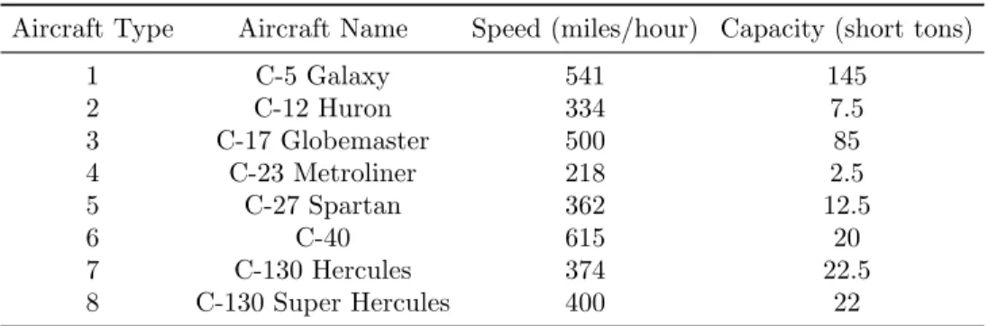
Data preprocessing. We first constructed a “master” set of ports. We assumed that this set consists of all possible United States Air Force (USAF) bases in the continental United States, leading to a set of 174 different airbases. For the aircraft, we assume that aircraft can be one of eight different cargo aircraft types used by the USAF. Figure 1 shows the distribution of ports in the continental United States, while Table 1 displays the eight different aircraft types, along with nominal values of their capacities and speeds. In the instances that we will shortly describe, aircraft travel times between pairs of events (the τe,e0_,a values) were calculated by computing the

distance between the latitude-longitude pairs using the haversine formula and converting this distance into a time via the nominal speed of the aircraft.

Problem instances. We consider two different sets of instances, described below: 1. T instances. In these instances, the data is generated as follows: