An experimental study of flame-wall interaction: temperature analysis near the wall

READ THESE TERMS AND CONDITIONS CAREFULLY BEFORE USING THIS WEBSITE. https://nrc-publications.canada.ca/eng/copyright

Vous avez des questions? Nous pouvons vous aider. Pour communiquer directement avec un auteur, consultez la première page de la revue dans laquelle son article a été publié afin de trouver ses coordonnées. Si vous n’arrivez pas à les repérer, communiquez avec nous à PublicationsArchive-ArchivesPublications@nrc-cnrc.gc.ca.

Questions? Contact the NRC Publications Archive team at

PublicationsArchive-ArchivesPublications@nrc-cnrc.gc.ca. If you wish to email the authors directly, please see the first page of the publication for their contact information.

NRC Publications Archive

Archives des publications du CNRC

This publication could be one of several versions: author’s original, accepted manuscript or the publisher’s version. / La version de cette publication peut être l’une des suivantes : la version prépublication de l’auteur, la version acceptée du manuscrit ou la version de l’éditeur.

Access and use of this website and the material on it are subject to the Terms and Conditions set forth at

An experimental study of flame-wall interaction: temperature analysis

near the wall

Tayebi, Badri; Galizzi, Cédric; Guo, Hongsheng; Escudie, Dany

https://publications-cnrc.canada.ca/fra/droits

L’accès à ce site Web et l’utilisation de son contenu sont assujettis aux conditions présentées dans le site LISEZ CES CONDITIONS ATTENTIVEMENT AVANT D’UTILISER CE SITE WEB.

NRC Publications Record / Notice d'Archives des publications de CNRC:

AN EXPERIMENTAL STUDY OF FLAME-WALL INTERACTION: TEMPERATURE ANALYSIS NEAR THE WALL

B. TAYEBI1, C. GALIZZI1, H. GUO2, D. ESCUDIE1

1

CETHIL Centre Thermique de Lyon, UMR 5008 CNRS-INSA-UCBL, INSA de Lyon, 9 rue de la physique, 69621 Villeurbanne Cedex, France

2

Institute for Chemical Process and Environmental Technology, National Research Council of Canada 1200 Montreal Road, Ottawa, Ontario, Canada K1A 0R6

ABSTRACT

In this study, the interaction between a premixed turbulent flame and a lateral wall is addressed. The objective is to correlate the modifications of the flame topology and the temperatures in the interaction zone. Laser tomography and thermal sensors are used in the experiment. Results show that the flame topology is modified along the flame front. The evolutions of the temperatures of the wall and the gases are shown to be more significantly influenced by the oblique shape of the flame front than by the curvature of the wrinkles.

1. INTRODUCTION

The understanding of flame-wall interaction in premixed combustion is a research area of continuous interest in many practical applications such as spark-ignition engines and gas turbine. Complex physical and chemical processes (aerodynamics, thermodynamics and chemical kinetics) are usually involved in flame wall interactions. Aerodynamic strain, boundary layer, heat transfers, thermal quenching, extinction and flame propagation are dominating phenomena during the interaction process. These phenomena have been intensively studied (Popp and Baum 1997, Foucher et al. 2003, Dabireau et al. 2003). The analysis of flame-wall interaction processes in industrial configurations is very complex. Alternately, the use of academic configurations appears to be a better solution if one wants to take insight into the way flame and wall interacts(Tayebi et al. 2008).

Poinsot et al. (1993) studied numerically the interaction between a turbulent premixed flame and a lateral wall. They observed that the process of the interaction is characterized by three effects: local conducto-convective thermal transfer, modification of the flame front topology and laminarization in the vicinity of the wall. Laminarization played a key role in the aerodynamic field in the interaction zone. The wall induced a modification of the flame topology and limited the spatial extension of the flame brush. The smoothing of the turbulent shape of the flame was pointed out in numerical study conducted by Alshaalan and Rutland (1998) as well as in the experimental results reported in Tayebi et al. (2007). Richard and Escudié (1997) investigated experimentally the interaction between a hydrogen-air flame and an adiabatic wall, for a mixture with Lewis number equal to 0.3. They defined an

interaction parameter as the ratio of the flame brush thickness to that of the boundary layer. For a fixed turbulent intensity (4%), they studied the evolution of the flame front length as a function of the interaction parameter. They observed three distinct interaction regimes. In the firstregime, the flame was deviated due to the deflection of the stream by the wall. In the second one, tongues of burnt gases appeared in the boundary layer and led to an increase of the length of the flame front. Finally, in the vicinity of the wall, the flame extinguished. Richard and Escudié justified the appearance of the tongues by an increase in the ratio of the flame speed over the boundary layer velocity. In the region of high shear. Kurdyumov et al. (2000) showed numerically that the Lewis number and the nature of the wall, adiabatic or isothermal, were important factors influencing the propagation of premixed flames near walls.

Many researchers have investigated the thermal aspect associated to the flame-wall interaction, particularly in the case of transient flames (Ezekoye et al. 1992, Bellenoue et al. 2003, Boust et al. 2007). However, only a few of studies treated the case of stationary flames. Alshaalan and Rutland (2002) studied the interaction between a stationary V-shaped flame and a lateral wall in a Couette flow configuration by three dimensional Direct Numerical Simulation (DNS). The turbulent flame and the wall were separated by a turbulent boundary layer. Results showed that the flame stretch increased and the wall heat flux decreased with decreasing speed streaks. In addition, they confirmed the results of Bruneaux et al. (1996) who postulated that the horseshoe vortex structures pushed the flame toward the wall and increased the wall heat flux. These authors justified the appearance of structures like “tongues” by the deformation of the flame wrinkles caused by the coherent structure, which are commonly encountered in turbulent boundary layers.

The aim of the present study is to improve our knowledge about the interaction process between a stabilized flame and a lateral wall. The influence of the boundary layer structure on the interaction process is addressed first, particularly the effects on the appearance of the “tongues” structures. Then, the topology structure of the turbulent flame front is studied. The use of an adiabatic wall instrumented with several thermal sensors allows the investigation of long time history of the wall and gases temperatures in the interaction zone before quenching.

2. EXPERIMENTAL SETUP AND IMAGES PROCESSING

2.1. Experimental setup and conditions

The configuration studied is shown schematically in Figure 1. A 2 mm diameter rod, set at the exit of a wind tunnel (115x115 mm²), ensures the stabilization of the flame. While the left front of the V shaped flame is free, the right front interacts with a vertical plate. The wall is made with a ceramic material that has a very low heat conductivity (λ=0.4 W.m-1.K-1). The wall is assembled on a support which makes it possible to turn, and invert the positions of the escape and leading edges. These two wall edges (Figure 2c) were designed in order to control the structure of the boundary layer.

When the wall is set up so that the acute edge is at the bottom, a laminar boundary layer is obtained. If the blunt edge is put at the bottom, the transition to a turbulent boundary layer is accelerated.

The leading edge of the ceramic plate was set at 50 mm downstream of the exit plane of the burner and the distance (d) separating it from the rod could be adjusted. Two references coordinates are used. The first one is linked to the wire (x, y) and the second to the leading edge of the plate (xw, yw). The main

purpose of these two coordinates systems is to define the single V-shaped flame, as usually done, independently of the boundary layer flowing on the plate.

The experimental conditions correspond to a lean premixed methane-air mixture with uniform velocity equal to 5 m.s-1 and an equilavence ratio equal to 0.61 at the exit of the wind tunnel. The turbulence was enhanced by a grid set at 50 mm upstream of the exit plane of the tunnel.

Fig. 1. The experimental setup.

Two thermal sensors were used to investigate the temperature in the flame-wall interaction zone. Each thermal sensor is made of two K type thermocouples. The first allowed us to obtain temperatures in the gases at 1 mm from the wall (Figure 2a) and the

second measured the temperature of the wall surface (Figure 2b). Thermocouples were inserted in a ceramic tubes made with a material similar to that of the wall in order to minimize heat flux discontinuity. The objective is to obtain temperature variation induced by the same flame wrinkle. For the wall region between xw = 88 mm and 132 mm, the mean

length of the wrinkles is 7 mm. Thus, the two thermal sensors were inserted respectively at the stations xw

= 120 and 126 mm from the leading edge of the wall (Figure 2c).

(a) (b)

(c)

Fig. 2. Thermal sensor and their position on the wall. To quantify the velocity field, Particle Image Velocimetry (PIV) was used. The flow was seeded with incense particles and illuminated with a laser sheet created by Nd:YAG (120 mJ) laser source and 3 lenses. The light scattered by the particles was recorded by a CCD camera PCO (1376 x 1024 pixels²). Velocities were determined by measuring the distance traveled by the particles between two consecutive laser pulses and dividing this distance by the interpulse time. In the present experimental configuration, each velocity vector was determined from the average particle displacement in 16 x 16 pixels² subregions, corresponding to spatial subregion of 0.352 x 0.352 mm².

2.2 Images processing

Laser tomography was used to study the topology structure of the flame front. Tomography of the flame

front shape and position were obtained by using the laser of the PIV system. In order to determine the instantaneous flame front position, each flame image was first normalized to account for laser sheet inhomogeneity. Then the image was analyzed with an edge-finding algorithm (Matlab software), and binary images for the burned and unburned regions were generated. These instantaneous images were then averaged to obtain “maps” of the mean progress variable (c) (Figure 3) and flame brush thickness (δT).

Fig. 3. c map for the right front of the free flame.

To access to the flame front length, the edge detected was then fitted with a polynomial curve. From this edge, a two-dimensional estimate of the flame surface density (Σ) was obtained, as it was expected by Veynante et al. (1994), as:

ds dL n

=

∑ (1)

where n is the number of images, dL is the infinitesimal flame front length contained in the surface element ds. For each image, the measured domain was divided into square boxes of 10 x 10 pixels² (1.7 x 1.7 mm²). In each box, the arc length of the flame front was computed (or is set to zero if no flame is present). Results were then averaged over 200 frames and divided by the box surface, leading to the flame surface density, and affected to the point located at the center of the box.

3. RESULTS AND DISCUSSION

3.1. The reference case: free turbulent oblique flame

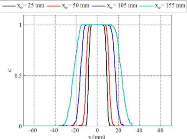
Figure 4 shows the profiles of the mean progress variable, where c = 0 corresponds to unburnt reactants and c= 1 corresponds to the burned products. The two regions (c = 0 and 1) are separated by the flame brush, whose thickness increases in the downstream direction. It also shows that for this free flame, the two oblique fronts remain symmetrical with respect to the stabilization rod set at y= 0 mm.

Fig. 4. Profiles of mean progress variable. The second characteristic of the flame analyzed is the flame surface density. A direct measure of this parameter (Lee et al. 2000) is possible using equation (1) and assuming that the oblique flame is two-dimensional. Figure 5 presents profiles of Σ at 4 stations downstream the flame holder. A fit of experimental results with the relation ∑=kc( −c) are also plotted. It shows a symmetric distribution of the flame surface density with respect to c= 0.5. The maximum of Σ decreases with increasing the distance from the flame holder. This means that the maximum of Σ decreases with increasing flame brush thickness, being consistent with the observation of Tang et Chan (2006).

Fig. 5. Profiles of the flame surface density.

3.2. Effects of the structure of the boundary layer on the flame wall interaction

Bruneaux et al. (1996) showed that for a three-dimensional flame-wall interaction, the boundary layer structure, particularly the coherent vortices, played a key role in the interaction process. The vortices induced the appearance of structure like “tongues” that increased heat losses toward the wall. Richard and Escudié (1997) observed the same phenomena in a two-dimensional configuration. As the Lewis number of the mixture used (Hydrogen-air

flame) was lower than unity (Le= 0.3), they justified the appearance of these structures by an increase of the flame speed in the regions of high sheer.

To examine if these two conclusions are sufficient to explain the appearance of these structures, we study in the present work a methane-air flame with a Lewis number equal to 0.98. The turbulent flame can be separated from the wall by a laminar or a turbulent boundary layer.

The results obtained in a previous study using LDA system (Tayebi et al. 2007) showed that the boundary layer was not modified by the flame when interacting with a turbulent flame.

The LDA technique enables to obtain a local and mean description of the aerodynamics and the use PIV leads to access to the maps of the aerodynamic field in the boundary layers. A close examination of the instantaneous fields is required to clarify the behavior of the flame in the velocity gradient region. The most important characteristic that makes the difference between the two boundary layer structures is the vorticity field, defined as:

y U x V z=∂_∂ −∂_∂ ω (2)

where ωz is the vorticity component along the z axis

(perpendicular to the x-y plane), and U and V are the two components of the velocity in x and y directions, respectively.

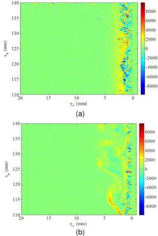
Figure 6 shows the vorticity fields in the boundary layers in the two situations. In the case of a laminar boundary layer (Figure 6a), a nearly homogeneous vorticity distribution along the boundary layer is observed. No coherent vorticity structure can be identified. On the contrary, in the case of a turbulent boundary layer (Figure 6b), coherent structures can be clearly identified. The vorticity amplitude changes from positive and negative values, pointing out the presence of contrarotating structures (Tomkins and Adiran 2003). The horseshoe vortices cause ejections of fluid from the wall to the external flow. Meanwhile, these ejections are equilibrated by bursts that push the external fluid toward the boundary layer.

Laser tomography was used to examine the behavior of the flame wrinkles in these fields. Figures 7a and 7b show tomographic visualizations of the flames interacting with a laminar and a turbulent boundary layer, respectively. We can clearly see that when the flame wrinkles are close to the wall, they are deformed and cause the appearance of structures like “tongues” for both laminar and turbulent boundary layers. This means that the velocity gradient is an important parameter that influences the propagation of the flame in a region of high shear, regardless the boundary layer type. As mentioned above, similar phenomena were observed by Richard and Escudié (1997), for a lean hydrogen-air mixture that has a Lewis number much less than that

of the current methane-air mixture, indicating that the phenomena is not directly related to Lewis number effect.

(a)

(b)

Fig. 6. Instantaneous vorticity field in the boundary layers. (a) laminar case; (b) turbulent case.

(a) (b)

Fig. 7. Tomographic visualizations of the flame wall interaction. (a) laminar case; (b) turbulent case.

Topology structure and flame surface density

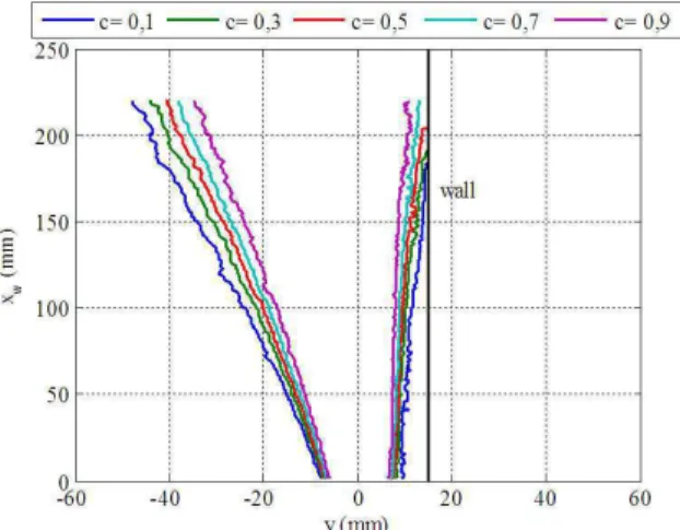
The tomographic visualizations presented in figure 7 show that the interaction between the flame and the wall induces a global deflection of the flame toward the direction opposite to the wall. This can be clearly seen on the isovalue of the progress variable

(c) given in figure 8. Moreover, this deflection is associated with a modification of the flame brush thickness which propagates from the interaction zone to the upstream region. This retroactive effect was not observed in the DNS calculations of Alshaalan and Rutland (1998).

Fig. 8. Isovalue of the mean progress variable. To examine how this smoothing influences the flame structure along the whole flame front in the interaction with the wall, two characteristic variables where chosen: the flame brush thickness (δT) and

the flame front length (L). We define a flame wall interaction parameter Ifw, as:

bl T fw / ' d I δ δ − = (3)

Where d’ is the distance between the mean flame front and the wall. Figure 9 presents the evolution of the flame brush thickness and the flame front length against the variation of Ifw. In order to quantify the

smoothing of the flame front, these two characteristics are adimensionalized by the characteristics of the free flame, i.e. δT0 and L0,

respectively. This figure shows that the interaction process can be divided into 3 zones. First, for values of the interaction flame wall parameter greater than 1 (Ifw>1), we can see that the wall limits effectively the

extension of the flame brush which is reduced compared to the free case (Poinsot et al. 1993, Alshaalan and Rutland 1998). The second zone corresponds to the region where the flame is in the boundary layer (Ifw<1). In this region, the brush

thickness still decreases, but the appearance of the tongues of burned gas induces a local increase of the flame front length, which confirms the results of Richard and Escudié (1997). Finally, in the last regime, the flame reaches the wall and extinguishes. In all these regions, as the flame front is confined by the wall, a drastic reduction of the flame brush thickness is induced before quenching.

Fig. 9. Flame front structure.

Figure 10 shows profiles of flame surface density, when the front is interacting with the wall. Compared to the case of the free flame (Figure 5), we can see that the maximum of Σ increases for all stations studied. Thus, the behavior of the flame structure appears to be correlated to the distribution of the flame surface density in the brush. The decrease of the flamelets amplitude is compensated by a modification of their spatial frequency, which causes an increase of the flame surface density, as the length is not reduced significantly (Tayebi et al. 2008).

Fig. 10. Flame front structure.

3.4. Effects of the interaction on the wall surface and gases temperatures

As it was addressed above, two thermal sensors (Fig 2) were inserted respectively at the stations 120 mm and 126 mm from the leading edge of the wall. The results presented in this section deal with the flame-wall interaction in the case of a laminar boundary layer.

The aim of the thermal analyses is to investigate how the topology of the flame wrinkles affects the variation of the wall surface and gases temperatures, before quenching. Temperature measurements were synchronized with laser tomographies. The

acquisition frequency of the visualization system is limited to 5 Hz. Acquisition time was taken equal to 60 s to investigate a long time variation history of the local temperatures. For the temperature measurements, the acquisition frequency is set equal to 500 Hz, and 100 temperatures are measured between two successive images.

Fig. 11. Evolution of the temperatures in the interaction zone. Tw1 and Tg1 are the data at xw = 120

mm and Tw2 and Tg2 are at xw = 126 mm.

Figure 11 plots the evolution of wall (Tw) and gases

(Tg) temperatures in the interaction zone. As the

flame is V-shaped, the distance separating it from the second thermal sensor is less than that separating if from the first one. Thus, the temperatures at the station xw = 126 mm are higher than that measured at xw = 120 mm. This temperature difference is significantly less at the wall surface than in the gases. Moreover, it is noted that some peaks of gases temperature exceed 300 °C. To investigate the physical mechanism responsible to these temperature jumps, the tomography visualization are analyzed.

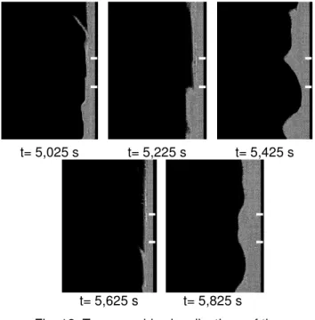
For the peak of temperature Tg1= 465 °C which

occured at t= 5.57 s, figure 12 gives five tomographic images acquired around this peak. On these inages, the two white marks correspond to the position of the two thermal sensors. It appears that for all the images, the wall and the flame are separated by a boundary layer of fresh gas (the white zone). As the fresh gas flows on the wall, the curvature of its surface varies from an image to another, since the flame is intermittent. This curvature induces a modification of the distance between the flame and the wall (d’). The curvature (h) can be defined by (Lecordier 1997):

(

)

where xɺ yɺxɺɺ and yɺ are, respectively, the first and ɺ second order derivatives of the flame coordinates relative the curvilinear abscissa.

t= 5,025 s t= 5,225 s t= 5,425 s

t= 5,625 s t= 5,825 s Fig. 12. Tomographic visualizations of the

temperature measurements region.

Fig. 13. Correlation of the flame characteristics and the temperatures beside the first sensor. For the first thermal sensor, figure 13 gives the variation of the flame curvature, the distance between flame and wall, and gases temperatures. Figure 15 plots the same quantities associated to the second sensor.

Between the second and the third images in Fig. 13, it appears that the flame topology undergoes an important change. Nevertheless, the corresponding temperatures in the gases are not modified. For the third image (t = 5.425 s), the flame curvature beside the first and the second sensor is respectively positive and negative. The flame is more close to the first sensor (d’ = 2.5 mm) than to the second (d’ =

5.45 mm) at this moment. However, the measured temperatures at these two locations are not modified by this curvature change. This means that the gases and the wall temperatures are not sensitive to this change in the flame curvature between the second and the third images.

Between the fourth (t=5.425 s) and the fifth (t= 5.625) images, the flame may be quenched at the wall, giving rise of the gases temperature up to 465 °C in a duration of 50 ms. This phenomenon is also detected by the second sensor but for a long duration (t = 210 ms).

Fig. 14. Correlation of the flame characteristics and the wall temperature beside the first sensor. This high jump of the gases temperature induces only a small wall temperature variation of about 5 °C (Fig 14), which can be explained by the very low thermal conductivity (λ= 0.4 W/m.K) of the wall. For the last image (t= 5.825 s), the flame is at 5 mm from the wall and its curvature is around zero beside both thermal sensors. The corresponding wall and gases temperatures are higher for the second sensor than for the first.

As the flame induces temperature gradients in the interaction zone, heat transfer must exist. Different mechanisms of heat transfer contribute to the heat exchange between the stabilized flame and the wall. However, the contribution of the convective heat flux (Qc) is the most important as the flame and the wall

are separate by a boundary layer. In fact, Qc is a

function of the temperature difference between the gases and the wall surface and can be expressed as:

(

)

c h T T

Q = − (5)

The heat transfer coefficient (h) varies with the distance from the leading edge, the gases velocity, and temperature, and can be correlated to the Nusselt

number: w xw x Nu h= λ (6)

where λ is the thermal conductivity. For a laminar boundary layer, the Nusselt number has been correlated with the following relationship (Incropera and Dewitt 1996): / / xw xw . Re Pr Nu = (7)

By using Eq. (6) and (7), the convective heat transfer coefficient around the two thermal sensors is 9.13 W/m².k.

Fig. 15. Correlation of the flame characteristics and the temperatures beside the second sensor. Figure 16 gives the evolution of the local convective heat flux around the two thermal sensors. For the first three images, as the wall surface is at a temperature higher than the surrounding fresh mixture, gases cool the wall. In addition, the local heat flux removed by the gases around sensor (1) is higher than around sensor (2). Between the third and the fourth images, the jump in the gases temperature induces a sharp increase of the heat transfer from the flame toward the wall.

CONCLUSIONS

The interaction between a turbulent flame and a lateral wall, separated by a boundary layer of fresh gas, was experimentally investigated. It is shown that when the flame is close to the wall, the velocity gradient causees the appearance of structures like “tongues” whether the boundary layer is laminar or turbulent. The use of laser tomography associated to image processing techniques show that the interaction induces a damping of the amplitude of the flame wrinkles and a modification of their spatial frequency. Before quenching, at the wall, the evolutions of the gas and wall temperatures show that the oblique shape of the flame is a more important parameter during the interaction than the wrinkles curvature.

REFERENCES

Alshaalan, T. and Rutland, C, J. (1998): “Turbulence, scalar transport, and reaction rates in flame-wall interaction”. Twenty-seventh Symposium (International) on combustion, The Combustion Institute, pp. 793-799.

Alshaalan, T. and Rutland, C, J. (2002): “Wall heat flux in turbulent premixed reacting flow”, Combustion Science and Technology, Vol. 174, pp. 135-165. Bellenoue, M. Kageyama, T. Labuda, S, A. and Sotton, J. (2003): “Direct measurement of laminar flame quenching distance in a closed vessel”,

Experimental thermal and fluid science, Vol. 27, pp. 323-331.

Boust, B. Sotton, J. and Bellenoue, M. (2007): “Unsteady heat transfer during the turbulent combustion of lean premixed methane-air flame : Effect of pressure and gas dynamics”., Proceedings of the Combustion Institute, Vol. 31, pp. 1411-1418. Bruneaux, G. Akselvoll, K. Poinsot, T. and Ferziger, J, H. (1996): Flame wall interaction simulation in a turbulent channel flow, Combustion and Flame, Vol. 107, pp. 27-44.

Dabireau, F. Cuenot, B. Vermorel, O. and Poinsot, T. (2003): “Interaction of flames of H2 + O2 with inert walls”., Combustion and Flame, Vol. 135, pp. 123-133.

Ezekoye, O. Greif, R. Sawyer, R, F. (1992): “Increased surface temperature effects on wall heat transfer during unsteady flame quenching”., In Twenty-Fourth Symposium (International) on Combustion, The Combustion Institute, pp. 1465-1472.

Foucher, F. Burnel, S. Mounaïm-Rousselle, C. Boukhalfa, M. Renou, B. and Trinité M. (2003): “Flame wall interaction : effect of stretch”.

Experimental Thermal and Fluid Science, Vol. 27, pp. 431-437.

Incropera, F. and Dewitt, D. (1996): “Fundamentals of heat and mass transfer”, Wiley Edition, Fourth Edition, 879 p.

Kurdyumov, V, N. Fernandez, E. and Linan, A. (2000): “Flame flashback and propagation of

premixed flames near a wall”, Proceedings of the Combustion Institute, Vol. 28, pp. 1883-1889.

Lecodier, B. (1997): “Etude de l’interaction de la propagation d’une flamme prémélangée avec le champ aérodynamique par association de la tomographie laser et de la vélocimétrie par image de particules”, PhD thesis., in French, Université de Rouen., 1997.

Lee, G. Huh, K. and Kobayashi, H. (2000): “Measurement and analysis of flame surface density for turbulent premixed combustion on a nozzle-type burner”, Combustion and Flame, Vol. 122, pp. 43-57. Nakamura, H. Igarashi, T. Tsutsui, T. (2001): “Local heat transfer around a wall-mounted cube in the turbulent boundary layer”. International Journal of Heat and Mass Transfer, Vol. 44, pp. 3385-3395. Popp, P. and Baum, M. (1997): “Analysis of wall heat fluxes, reaction mechanisms and unburnt hydrocarbons during the head - on quenching of laminar methane flame”, Combustion and Flame, Vol 108, pp. 327-348.

Poinsot, T, J. Haworth, D, C. and Bruneaux, G. (1993): “Direct simulation and modeling of flame-wall interaction for premixed turbulent combustion”.

Combustion and Flame, Vol. 95, pp. 118-132. Richard, G. and Escudié, D. (1997): Experimental study of a premixed flame interacting with a wall.

Proceedings of the Second Symposium (International) on Turbulence, Heat and Mass Transfer, pp. 651-663.

Tang, B, H, Y. and Chan, C, K. (2006): “Simulation of flame surface density and burning rate of premixed turbulent flame using contour advection”.

Combustion and Flame, Vol. 147, pp. 49-66.

Tayebi, B. Galizzi, C. Leone, J,-F. and Escudié, D. (2007): “Experimental Study of the flame-wall interaction”. Third European Combustion Meeting, Crete ,11-13 April.

Tayebi, B. Galizzi, C. Leone, J,-F. and Escudié, D. (2008): “Topology structue and flame surface density in flame wall interaction”, Eurotherm, Eindhoven , 18-22 May.

Tomkins, C, D. and Adiran, R. (2003): “Spanwise structure and scale growth in turbulent boundary layers”. Journal of Fluid Mechanics, Vol. 490, pp. 37-74.