DIC Challenge: Developing Images and Guidelines for Evaluating
Accuracy and Resolution of 2D Analyses
P. L. Reu
1a, E. Toussaint
b, E. Jones
a, H. A. Bruck
c, M. Iadicola
d, R. Balcaen
e, D. Z. Turner
a,
T. Siebert
f, P. Lava
g, and M. Simonsen
ha
Sandia National Laboratory, Albuquerque NM, USA
b
University Clermont Auvergne, France
cUniversity of Maryland, USA
d
National Institute of Standards, Gaithersburg, MD, USA
eKU Leuven, Ghent, Belgium
f
Dantec Dynamics GmbH, Ulm, Germany
gMatchID, Ghent, Belgium
h
Correlated Solutions Inc., Columbia, SC, USA
Abstract
With the rapid spread in use of Digital Image Correlation (DIC) globally, it is important there be some standard methods of verifying and validating DIC codes. To this end, the DIC Challenge board was formed and is maintained under the auspices of the Society for Experimental Mechanics (SEM) and the international DIC society (iDICs). The goal of the DIC Board and the 2D-DIC Challenge is to supply a set of well-vetted sample images and a set of analysis guidelines for standardized reporting of 2D-DIC results from these sample images, as well as for comparing the inherent accuracy of different approaches and for providing users with a means of assessing their proper implementation. This document will outline the goals of the challenge, describe the image
sets that are available, and give a comparison between 12 commercial and academic 2D-DIC codes using two of the challenge image sets.
Keywords: Digital Image Correlation, DIC, metrology, full-field measurement
1. Introduction – Description and goals of the challenge
Digital image correlation (DIC) is a full-field image based method of measuring displacement and strains proposed and established for two-dimensional measurements in the 1980s [1-3], and for three-dimensional measurements in the 1990s [4,5]. For a full description of the algorithms and implementation of DIC we direct the reader to the seminal book by Sutton [6]. This paper only contains a brief review of DIC in a nontechnical context to orient a reader to the basic ideas of 2D-DIC. The paper then focuses on the DIC Challenge images, their creation and purpose, and a discussion of the results of the first DIC Challenge.
1.1 Local DIC formulation
The fundamental principle behind local DIC is to subdivide an image into small, individually resolved subsets (facets). The subsets are then each analyzed to measure the motion and deformation between integer pixel locations in the selected reference image and any deformed images. To resolve grey level values at sub-pixel locations in the deformed image, interpolation schemes are used to reconstruct the image. Most 2D-DIC software solves a nonlinear minimization function using the grey levels to find an optimum match. During this process the subset is allowed to deform by means of the subset shape function and the grey levels are interpolated for a subpixel match [7]. Various minimization formulations may be used to find the optimum match, for example the Sum of the Squared Differences (SSD) formulation (see the article series in Experimental Techniques [8] for a more complete outline of basic DIC methods from a practical viewpoint). The software then reports the found location of the subset in the deformed image. Added information may also be available at other inter-subset locations from the subset shape function, but is nearly always left unused. Many commercial code details are not documented or explained because of intellectual property concerns, although most employ the basic principle presented here. Consequently, many practitioners must use their software as a “black box”. We direct the reader to the vendor’s software documentation or papers published by the university codes when available for details about the implementation of specific software packages.
1.2 Global DIC Formulation
Unlike local DIC, global DIC solves for the displacement field between the reference image and the deformed images for all points within the image simultaneously. To do this, the image is discretized with a finite element (FE) mesh, and then the displacement field is found by minimizing the grey level differences. The result is the nodal point motion. Results are found at other locations in the image using the FE shape functions. We direct the reader to Hild and Roux for more details on global DIC implementation [9]. Therefore, in principle, global and local DIC are very similar, except for the reconstruction approach to the deformed image and subsequent number of pixels used to correlate with the undeformed image.
1.3 Design and Purpose of the DIC Challenge
The DIC Challenge is in large part inspired by the Particle Image Velocimetry (PIV) challenge and is following a similar, although slower, course [10-12]. The goal of the DIC Challenge is not to decide which DIC code is best, but rather to provide a venue where codes can be verified, tested, vetted and discussed to help standardize analysis of their inherent accuracy and to help users properly employ them. Towards this end, the DIC Challenge Board carefully designed image sets to test problematic areas in DIC analysis. These include:
• Interpolation bias errors due to improper selection of interpolants.
• Inability to deal with sample rotation (as is the case in the frequency based methods). • Robustness to image noise and/or lack of image contrast.
• Determination of the ideal balance between smoothing and spatial resolution.
The DIC Challenge images and accompanying analysis algorithms provide a standard for evaluating the accuracy and precision of DIC software. This toolbox has several applications:
1. Journal publications claiming improvements in the accuracy of DIC algorithms.
2. Investigation of commercial software to allow users to better understand the DIC “black box.” 3. Code verification.
4. Comparisons between multiple DIC codes, for example local and global formulations.
An exercise like the DIC Challenge would not be complete without a “competition portion”. For the competition, each commercial vendor or code-developer ran their own software using the provided sample images, which removed the possible problem of “inexpert” users. The vendors then reported their results to the DIC Challenge Board, and the results were analyzed using a common set of algorithms. We draw two main conclusions from this
functions, etc., when run by an expert user, nearly all the codes analyzed for this paper returned essentially the same results. Second, the competition raised an important discussion that is a fundamental problem with DIC: the trade-off between spatial resolution and filtering of the data. A cautionary note is that users often prefer to have a smoother result, as it looks better to the human eye; however, this may not be the optimum result for a given use of the data. Both of these conclusions emphasize the need for training of DIC users.
1.4 Important definitions
Definitions are important when discussing measurement uncertainty. The DIC Challenge board follows the guidelines laid out in the Bureau International des Poids et Mesures (BIPM), an international body that helps define measurement standards and terminology. Two definitions from the BIPM vocabulary document are particularly important for this paper: Precision and Accuracy [13]. “Measurement Precision” is defined as the “closeness of agreement between indications or measured quantity values obtained by replicate measurements on the same or similar objects under specified conditions. “Measurement Accuracy” is defined as “closeness of agreement between a measured quantity value and a true quantity value of a measurand.” In the context of this document, the measurand is the displacement in pixels at locations in the image. Strain is a derived quantity from the displacement measurand. “True quantity value” has a particular meaning and is often unknowable in practical situations. However, with synthetic images, we have a true value, and this is used in comparisons. “Resolution” is defined as “smallest change in a quantity being measured that causes a perceptible change in the corresponding indication.” This term is used more colloquially in this document to indicate displacements that are measurable above the noise floor and is related to precision and the measurement noise in this sense. A final term “Spatial Resolution” is specific to DIC and is defined as the inverse of the cutoff frequency at some given decrease in signal.
1.5 Paper content and organization
The article is organized into three main sections. The first section briefly describes the image sets and the goals of the DIC challenge, including details on how we created the synthetic images and the relevant references. Appendix A contains example analysis of all the sample images and some typical DIC results obtained for them. The second section picks two image sets that the participants analyzed (Sample 14 and 15), describes the image sets and methods of analysis, and presents the results of the first challenge round. The final section in the paper
presents conclusions and future goals of the DIC Challenge. The website includes information on the MatLAB and LabVIEW analysis codes2.
2. DIC Challenge Image Sets
Table 1 lists the DIC Challenge image sets available at the website https://sem.org/dic-challenge/ at the time of publication. We developed nineteen image sets, including rigid-body sub-pixel translations, rigid-body rotations, out-of-plane translation, spatially-varying displacement and strain gradients, and displacement discontinuities. Each image set seeks to challenge one or more characteristics of DIC analysis, such as interpolation bias, robustness to image noise, ability to account for rotations, and determination of the balance between spatial smoothing and spatial resolution. The numbering scheme of the image sets was arbitrarily created. However, we preserve this numbering scheme for existing journal articles that refer to this historical naming convention. Image sets 1 - 13 and 16 - 17 serve two main purposes. First, the image generation processes were thoroughly vetted by a large cadre of DIC practitioners, which settled questions about the image creation and appropriateness for use in assessing DIC codes. Second, these image sets allow DIC code developers and users to verify3 and
evaluate basic performance of their software. Towards this end, we provide the standard analysis algorithms for the results on the website. We also provide example analyses using a single, commercially-available DIC software in the supplementary information in Appendix A. Authors of publications describing new DIC algorithms or software are strongly encouraged to verify and evaluate their codes using these image sets and standard data analysis algorithms, with proper referencing, and present the results in their publication. The standard analysis algorithms also make comparisons between different codes straightforward. The use of standard images and analysis algorithms will provide an even playing field and a more easily reviewed paper when claims of 2D-DIC improvements are made.
For most well-implemented and fully-developed DIC codes, obtaining reasonably accurate results from samples 1 – 11, 16-17 is trivial. Therefore, two more image sets – Sample 14 and Sample 15 – were generated with the intention to challenge DIC capabilities, specifically probing the relationship between noise suppression and spatial
2 Certain commercial equipment, instruments, or materials are identified in this paper in order to specify the
experimental procedure adequately. Such identification is not intended to imply recommendation or
endorsement by the National Institute of Standards and Technology, nor is it intended to imply that the materials or equipment identified are necessarily the best available for the purpose.
filtering. We discuss the analysis of these images by all participants of the DIC Challenge in the DIC Challenge Results section.
Table 1. Sample image set numbering and information. Image sets are available at: https://sem.org/dic-challenge/.
Description Set Name Method
[15,16] Contrast Noise σ (GL) Shift (pixels) # Images TexGen Shift X,Y Sample1 TexGen Varying 1.5 X=Y=0.05 20
TexGen Shift X,Y Sample2 TexGen 0 to 50 8 X=Y=0.05 20
FFT Shift X,Y Sample3 FFT Shift 0 to 200 1.5 X=Y=0.1 10
FFT Step Shift Sample3b FFT Shift 0 to 200 1.5 0.05 to 0.5 5
FFT Shift X,Y Sample4 FFT Shift 0 to 50 8 X=Y=0.1 10
FFT Shift X,Y Sample5 FFT Shift Varying 1.5 X=Y=0.1 10
Prosilica Bin Sample6 Binning 0 to 200 0.26 X=Y=0.1 10
Prosilica Bin Sample7 Binning 0 to 50 0.66 X=Y=0.1 10
Rotation TexGen Sample8 TexGen 0 to 100 2 Θ by 1 10
Rotation FFT Sample9 FFT 0 to 100 2 Θ by 1 10
Strain Gradient Sample10 TexGen 0 to 200 2 Sinusoid 10
Strain Gradient Sample11 TexGen 60 to 130 2 Sinusoid 10
Strain Gradient Sample11b FFT 0 to 200 1.5 Tri. .01 to 1 6
Ex1 – Plate Hole Sample12 Exper. Good Low N/A 12
Ex2 – Weld Sample13 Exper. Poor Low N/A 52
Varying Strain Sample 14 FFT 0 to 200 5 N/A 4
Varying Strain Sample 15 TexGen 80 to 180 2 N/A 9
Rigid Motion Sample 16 Exper. 0 to 254 0.26 ≈0.1 11
Interpolant Sample 17 Exper.
3. Image Generation Methods
The images in the DIC Challenge were created by one of four means; two synthetic methods, one pseudo-experimental method and one pseudo-experimental method. Synthetic images serve the purpose of providing a known solution against which DIC results can be compared, and their use is important for verification of the DIC software. Note that it is not possible to discover the experimental DIC uncertainty using only synthetic images. There are too many missing error sources and biases (e.g., spatial variations in illumination, pixel noise, and optical distortions) in the synthetic images to draw conclusions about any given experimental setup. Therefore, we also include pseudo-experimental and purely experimental image sets. While there are no known, exact solutions for these experimental image sets, results from different DIC codes and from a single DIC code run with different settings can be compared.
3.1 Synthetic image generation
The two methods of synthetic image generation used in the DIC challenge are the TexGen Software and the Fourier method. The TexGen software is documented in [16], which describes the mathematical approach used
for creating “semi-realistic” images. TexGen is useful in that it uses analytical functions to define a speckle field which can then be sampled to create a deformed image. A drawback is that “real” speckle patterns cannot be used, making it impossible to evaluate problems that may be caused by the applied speckle characteristics. To work with experimental speckle patterns, we used a second method that exploits the properties of the Fourier transform expansion or the Fourier phase shift to create deformed or shifted images, as explained in [15]. Fourier methods have the advantage of allowing real speckle images to be used but use a different method of interpolation than that used by the DIC codes. In fact, Fourier shifting uses the ideal sinc interpolant function, but without having an infinite image size. The sinc function results in the most accurate interpolation possible, given the underlying data [17,18]. All other DIC software interpolants use a smaller support (region of the image) for the interpolant and are therefore some approximation of the ideal sinc interpolant. The bi-cubic spline is one well-known example used in many DIC codes. The DIC codes require this approximation for speed and spatial resolution considerations that do not occur when creating synthetic images. It is important to consider the influence of the synthetic image generation on the calculated results from DIC. This topic has been treated in [19] with the conclusion that the FFT and TexGen method can be used for determining what they term is the “ultimate error regime,” i.e. errors caused only by the numerical DIC process interacting with image contrast and noise, but without other parasitic experimental errors. This is termed “verification” in this document.
Table 2 provides typical image noise for several types of machine vision cameras, as measured experimentally by acquiring five or more images of a completely stationary speckle pattern method. Completely stationary was obtained using an optical table and acquiring the images over only a few seconds. The pixel by pixel noise is then calculated and combined for the entire image to calculate the standard deviation of the grey values and the percent noise. Percent noise is calculated by dividing the measured noise standard deviation by the camera grey level range, 256 counts for an 8-bit image. For both the Fourier and TexGen synthetic images, image noise can be added to mimic camera noise. For these images, homoscedastic Gaussian noise was added of a given magnitude, as specified in Table 1. The image noise is specified as one standard deviation (1σ) of the grey level applied independently to each pixel. This is an approximation of the heteroscedastic noise profile of a typical machine vision camera [20]. Heteroscedastic noise scales with the pixel intensity, although still Gaussian in distribution. That is, brighter pixels have more noise than darker pixels in a generally linear fashion and can be measured using a grey card with a distribution of intensities and calculating the noise at the different intensities. Future simulations should take this fact into account. We assume that any discrepancies in the images between using a homoscedastic and heteroscedastic noise model will be small, although this remains unproven.
Table 2. Typical machine vision camera noise levels
Camera (8-bit) %Noise StDev (counts)
PointGrey GRAS (5MP) 0.82 1.56 PointGrey GX (5MP) 0.46 1.17 AVT Prosilica GX (5MP) 1.7 4.1 Prosilica GE4900 (16MP) 0.86 0.34 Prosilica Binned (0.1MP) 0.1 0.28 Phantom v611 (1MP) 0.78 1.84 Andor Neo (5MP) 0.60 1.51
3.2 Pseudo-experimental image shifting
We adopted a “super-resolution” approach as outlined in [15] to move closer to experimentally created images, but still with exact subpixel shifting. In brief, this technique uses a 16-Megapixel (4872 × 3248 pixels2),
high-resolution camera with oversized speckles of 50 pixels. The image is then numerically binned, by averaging 10×10 “super-pixels” into a single pixel to create a lower resolution image of 487 × 324 pixels2. After numerical binning,
the speckles are then a suitable size of 5 pixels. Then by changing the first binning row or column of the full-resolution image from index 0 to 9, we achieve an exact subpixel shift of the binned pixel of 0.1 pixels. Pseudo-experimental shifting has the advantage of making no assumptions about how the camera hardware captures the image and it is therefore closer to an experimentally shifted image. Other researchers have adopted the super-resolution image creation to minimize the influence of interpolation during synthetic image generation [21].
3.3 Experimentally generated images
Experimentally created images do not have the questions of authenticity that synthetic images have; however, knowing the “true value” for comparison with a DIC result is difficult or impossible. Experimental images have two uses: First, as a comparison between DIC codes or different settings within the same code. And second, as a comparison with a ground truth secondary measurement as in Sample 16 with rigid body motion, where the position is known to subpixel accuracy using an optical encoder on the stage.
3.4 Other image details
All images are monochrome 8-bit tagged image file format (*.tif or *.tiff). We chose 8-bit images because it has been shown that higher bit count does not noticeably improve the DIC results [22,23], therefore results using 10-bit or higher images would not change any conclusions. Rather, the magnitude of the matching error is proportional to the ratio of image contrast to image noise [23]. The DIC Challenge explores this relationship in all the image sets by varying the image contrast and the noise level. In practice, the connection between the noise and contrast also scales with camera bit depth, lessening the advantage of greater than 8-bits for DIC, all other
experimental parameters being equal (ignoring some experimental niceties). Each sample directory provides either a comma separated text file (*.csv) or spreadsheet file that contains information pertinent to the image set, whether that be the shifting or deformation profiles or the displacement is encoded in the image filename. This information provides the user with the known solution, against which DIC results can be compared for code verification.
4. Description of Image Sets for Code Verification
This section describes image sets 1-12 and 16-17 provided for basic DIC code verification. Analysis of these sample images are in Appendix A with a brief discussion of the expected results. Standardized analysis algorithms are provided on the website.
4.1 Sample 1 and Sample 5 (Shifted image with varying contrast using TexGen and FFT)
Sample 1, and 5 are both rigid body shifted images with constant noise (standard deviation of 1.5 counts grey level in an 8-bit image) and varying contrast. We created Sample 1 using TexGen and Sample 5 using the Fourier method. The images are shifted in both x- and y-directions simultaneously in increments of 0.05 pixels/step (Sample 1 – see Appendix A, Figure 17) and 0.1 pixels/step (Sample 5 – see Appendix A, Figure 18). Figure 1 shows the first and last image histogram for Sample 1. Sample 1 provides a varying contrast throughout the image series. Most DIC codes cannot correlate the entire series unless a Zero-Normalized Sum of Squared Differences (ZNSSD) algorithm is used because the contrast shift is different for each image. It is important for DIC codes to compensate for contrast changes over time because in many DIC experiments, particularly for stereo-DIC, there will be changes in the contrast during the experiment.
Figure 1. Histograms for first and last image of Sample 1 showing the change in contrast and saturated pixels for image trxy_s2_20.tif.
4.2 Sample 2 and Sample 4 (Shifted images with extremely high noise using TexGen and
FFT)
Another significant challenge for DIC is noisy images. Noisy images are not common with traditional machine vision cameras, but can be prevalent in alternative imaging methods, including x-ray, atomic force microscope, scanning electron microscope, ultra-high-speed cameras, and so forth. For example, the Sample 2 and Sample 4 image sets have an applied noise with a standard deviation of 8 counts and a fixed contrast spread of 50 counts. Sample 2 was created using TexGen, and Sample 4 using the Fourier method. Figure 2 shows just how poor these images are, with the noise being obvious in the image.
Figure 2. Histogram equalized plot of a small region of the image showing the obvious noise and the speckles. Corresponding histogram shows the small range of contrast available for matching by the DIC algorithm.
4.3 Sample 3 and Sample 3b (FFT Shifted image)
Sample 3 and Sample 3b are examples of good contrast and low noise images shifted using the FFT function. Sample 3 is a rigid body shift of 0.1 pixels per image and will nicely reveal both the DIC interpolation bias and variance. Sample 3b uses the same FFT shift, however, only the bottom half of the image is shifted. Sample 3b can be used to look at the effect of discontinuities in the results and the roll-off of the DIC filtering by applying a step function.
4.4 Sample 6 and Sample 7 (Pseudo-experimental rigid body shift with low and high noise
floot)
Sample 6 and Sample 7 were created using a 16-Megapixel ultrahigh resolution camera image and the super-resolution approach discussed in [15]. Sample 6 represents a high-contrast-low-noise image created experimentally and shifted via binning. This is as close to a completely experimental, perfectly-subpixel shifted
image as is possible. The binning was the only numerical processing done; neither the contrast nor the noise was changed. Typical noise levels for machine vision cameras are 1 to 2 counts, as shown in Table 2. The noise present in the image of Sample 6 of 0.26 counts is low for a machine vision camera because of the 10-pixel binning which suppresses the noise by a factor of 1/sqrt (N), where N is the number of binned pixels. Therefore, in general this is a lower image noise than would be encountered in a traditional non-binned machine vision camera. Sample 7 has a higher noise floor of 0.66 counts, which we experimentally obtained by increasing the gain of the camera to increase the image noise rather than adding noise in after the binning. The unbinned image had 5.5 counts of noise. The binning procedure used in Sample 7, even with a high gain on the raw image, results in an image noise that is still modest for a machine vision camera. Additionally, the contrast range in the experimental image was sub-optimal in Sample 7 to exacerbate any matching errors in the DIC analysis.
4.5 Sample 8 and Sample 9 (Rigid body rotation using TexGen and FFT)
Samples 8 and 9 were created to test a potential flaw in DIC codes in how they deal with rigid body rotation. In early codes, inaccurate displacements caused by image rotations were inherent in the simple frequency based cross-correlation methods used. In spatial-minimized codes, problems with the shape function may also result that create bias errors when the sample rotates. We created Sample 8 using the TexGen software and Sample 9 using an FFT rotation method [24]. Both samples are a rigid body rotation from 0˚ to 10˚ in 1˚ increments about the image center without any deformation. Both images have approximately 100 counts of contrast and an image noise of 2 counts (1σ).
4.6 Samples 10, 11 and 11b (Simple strain gradients using TexGen and FFT)
Samples 10, 11 and 11b were created to have a simple strain gradient variation across the sample. Samples 10 and 11 were produced with TexGen using the quasi-sinusoidal function from Fazzini [25]. The 10 images have increasing magnitudes of the same function. The two samples are different in that the contrast range for Sample 11 is only 70 counts while Sample 10 has 200 counts.
Sample 11b is a triangle displacement field created using a Fourier expansion by 100 and then a linear interpolation to find the grey value at the shifted pixel location. This creates a discontinuity in the strain field, which helps to probe the spatial resolution of the DIC package. In signal processing terms, this is equivalent to putting a strain level step function into the DIC “filter” and looking at the roll-off.
4.7 Sample 12 and Sample 13 (Experimental results from a tensile test on a hold and weld)
Sample 12 is a purely experimental data set using a painted speckle pattern on a tensile specimen with a hole in the middle. A publication by Passieux [26] used these images and more details are available there. As this is an experimental image series, there are no ground truth data for comparison with the DIC results. This data is useful for virtual strain gage size studies into the spatial resolution and noise robustness of DIC codes, as well as round-robin type tests for comparing one code versus another code of different DIC formulations (global versus local for example).
Sample 13 is included as an example of more “difficult” experimental imaging conditions. The data is from a 2D experiment using a ring light and bead-blasted surface preparation. The purpose of the experiment was to characterize laser welds in 304L stainless steel [27]. The advantage of using the bead-blast created surface contrast in the experiment is there was no paint debonding at the high strain values. This choice however introduces a problem of “evolving” speckles during the test. It is therefore difficult to run this analysis without using incremental correlation. A larger number of images (52) is provided to minimize the difference in speckle appearance between any two images in the series. The speckles are also most likely aliased, which introduces another error source and a particular challenge for certain interpolants (e.g. bilinear). However, the strains are large providing a good signal to noise ratio. The weld is near the middle of the sample, as indicated by a small black line on the right edge of the sample as labeled in Figure 3.
Figure 3. Reference image from Sample 13 showing the questionable speckle quality and the weld location. Speckles are created by using a ring light
4.8 Sample 16 (Experimental results for in-plane, rigid body translation)
To explore interpolation error, we acquired “exact” subpixel shifted experimental images using an Aerotech nm-precision displacement stage and a Prosilica 16-MPixel camera with a Nikon 28-85 mm zoom macro lens (see Figure 4). The speckle pattern was approximately 50 pixels in the full resolution image. The image was then decimated by a factor of 10 as described in [15] to yield speckles that were roughly 5 pixels in size. Note that the sample was shifted mechanically by moving the stage, rather than the pseudo-experimental method discussed previously. The binning was used purely to decrease the image noise. The binning approach has two benefits: First, it makes the stage step size 10× larger on the object, improving the displacement resolution of the stage by a factor of 10. Second, it improves the noise profile of the camera from σcounts = 0.86 grey levels down to about
σcounts = 0.26 gray levels. To improve the noise even more, 5 images at each stage position were averaged, after
first being binned, to yield a single image for analysis. We moved the stage in 33.5 micron steps, which corresponded to 0.1 pixels per step, for 10 steps. The stage encoder measured the true position at each step to have a secondary “known” measurement of stage motion against which DIC results can be compared. The vendor calibrated stage had an absolute position accuracy of ±280 nm over the entire 160-mm travel range, which corresponds to +/- 0.0008 pixels. The vendor stated position resolution should be even better over the 0.33 mm travel used for this subpixel shift.
Figure 4. Experimental setup for Sample 16. Prosilica 16 Megapixel camera and Aerotech stage used for in plane translation.
A second, cheaper and simpler approach to explore interpolation error was designed, and the experimental setup is presented in Figure 5 (compare this with the experimental setup used for Sample 16). A speckle pattern adhered to a manual linear stage was translated out-of-plane, perpendicular to the camera axis. Out-of-plane motion towards the camera of several millimeters generates effective sub-pixel in-plane expansion. Therefore, a simple manual stage has sufficient displacement resolution to provide accurate “known” applied displacements. This simple setup can be used to probe the quality of the interpolant and to discover the magnitude of interpolation errors relative to variance errors. While experimental data is available on the DIC Challenge website, this tabletop experiment can easily be replicated. The Field of View (FOV) was roughly 100-mm with a Point Grey 5-Megapixel Grasshopper camera and an Edmund Optic 35-mm lens.
Figure 5. Sample 17 out-of-plane translation experiment. Note that a manual stage will work as well. Floating optical table is not required.
5. DIC Challenge Results
5.1 Selection of images for challenge participants
After thorough vetting of the image generation process by the participants using Samples 1 through 11, Samples 14 and 15 were generated and provided for analysis to the challenge participants. In this round of the Challenge, participants were also provided with the exact solution. These images were designed to probe the connection between displacement and strain noise suppression and spatial filtering in the DIC analysis, a balance that every DIC user must make in every DIC analysis. The participants were only allowed to submit one set of results for analysis. A future blind study may include the possibility to provide two different results to illustrate the trade-off between spatial resolution and filtering within one DIC formulation.
For this preliminary study, 9 participants elected to provide results to the DIC Challenge board. They included five commercial vendors (all existing vendors at the time), three university codes and two global codes. The results were submitted as a text based delimited file with the displacements and strains reported at a 5-pixel spacing over the entire image area. Table 3 lists the participants, type of code and name of the 2D-DIC software used for the analysis. We do not reveal the correspondence of the codes/vendors and the results in this paper. We desire in a future blind study that includes a broader cross-section of participants to include the names of the participants with the results. However, at this point in the Challenge, anonymity was useful to encourage participation, mitigate fears, and allow for open discussion on how to “score” the images.
To score the quality of the results is a difficult task, fraught with the dual challenge of analyzing the entirety of the full-field results, while simultaneously deciding metrics on which to score them. This task is even more challenging when using a single set of results to determine quality: Does the participant choose to reduce noise, but at the expense of increasing bias errors, or try to capture the peak, but at the expense of increased noise? The answer to the question of balancing noise and bias error with spatial resolution is dependent on the data use. Therefore, “scoring” will always be subjective. However, this preliminary study did prompt discussion and an understanding of how to quantify the spatial resolution of DIC. This paper seeks to disseminate that information to a wider audience to help provide a means for evaluating DIC software in other journal publications.
Table 3. List of DIC participants
Participant Code Description Code Type
Elizabeth Jones MatLAB Code Local, subset based
Stephane Roux/François Hild Previously a university codehttp://www.correli-stc.com/ CorreliSTC – Global
Daniel Turner Sandia National Laboratory Code https://dice.sandia.gov/ DICe – Global DICe – Local Pascal Lava/Lukas Wittevrongel Previous university code http://www.matchidmbc.com/ MatchID – Local AdaptID - Global Micah Simonsen Correlated Solutions Commercial Codehttp://correlatedsolutions.com/ Vic2D – Local Thorsten Siebert Dantec Dynamics Commercial Codehttp://www.dantecdynamics.com/ Q-400 Istra4D Bernd Wieneke LaVision Commercial Codehttp://www.lavision.de/ StrainMaster DIC Markus Klein/Tim Schmidt GOM and Trilion Commercial Codehttp://www.gom.com/ ARAMIS
Remember: The goal of the Challenge is to provide a venue where the DIC community can come to compare and improve their DIC codes and discuss critical topics such as “spatial resolution” and how to quantify and to understand the DIC results. We do not seek to create a hierarchy of DIC codes. The images will be available for future developers and users of DIC code who utilize these standard images to test their code and learn about using DIC software.
5.2 More detailed description of image sets provided to participants
5.2.1 Sample 14 (Spatially varying sinusoidal displacement field)
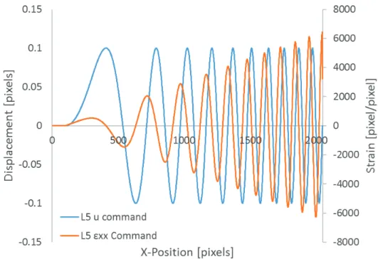
Sample 14 was created using a standard FFT expansion of the image by a factor of 100. This super-resolution image was then linearly interpolated to find the grey value at the subpixel location, using a displacement field, Ux(x), defined by the function in Eq. 1.
𝑈𝑈𝑥𝑥(𝑥𝑥) = 2𝜋𝜋𝜋𝜋 cos �2𝜋𝜋𝑥𝑥𝑝𝑝 � Equation 1
where p and α are the relative period and the amplitude, which can be varied to create a varying frequency and constant amplitude sine wave. The images were created with a constant displacement amplitude indicated in the filename and results file; however, this creates a varying strain amplitude throughout the image (see Figure 6). Future image sets will include both constant strain amplitude and constant displacement amplitude images to explore the filtering trade-off in both spaces separately and equally.
Several different noise levels were explored during the development of the images, including noise varying between 0 through 5 counts. While 5-counts of noise is high for a machine vision camera (between 1 and 2 counts is more typical, c.f. Table 2), we chose the higher level to better explore the key trade-off between spatial filtering and noise in the displacement and strain fields. A noisier image will worsen the displacement and strain noise, requiring the user to select a balance between more filtered results (for example with a larger subset or strain window) versus better spatial resolution.
Note that this function is in an Eulerian coordinate system and needs to be corrected to a Lagrangian coordinate system for comparison with the DIC results. This detail is true both of the FFT Sample 14 images and Sample 15 TexGen images, and is discussed in Section Euler versus Lagrange.
Figure 6. Commanded displacement and strain field for “Sample 14 L5 Amp0.1.tif”. Commanded displacements and strains are identical for all x-rows in the image.
5.2.2 Sample 15 (Spatial varying displacement field with discontinuities)
Sample 15 complements the results from Sample 14 by providing a displacement field with sharp discontinuities. This tests the spatial resolution similarly to many cases found in common DIC experiments, for example, grain boundaries, material cracks, etc. Sample 15 was created using the TexGen software. While Sample 14 used a real experimental image as the basis, Sample 15 is a synthetically generated image. Sample 15 varies the displacement in the vertical direction. The displacement profile is available at the pixel locations in the associated data file. Figure 7 shows an example of the strain profile from the results for both the full-field results and the line cut profile of the displacement and strain.
Figure 7. Sample 15 k250 commanded displacement and strain field. Commanded strain is identical for all y-columns in the image. Color plot is the full-field strain εxx.
5.3 Euler versus Lagrange: An important detail
Both Sample 14 and Sample 15 were plagued in the early rounds of the challenge with having the “measured” DIC results and the “known” synthetic displacement field in different coordinate systems (i.e., the commanded displacements are naturally in Eulerian coordinates, while the DIC results are naturally in Lagrangian coordinates). An accurate analysis requires the transformation into a common coordinate system. The coordinate system issue is an important but subtle point in image generation, and stresses the need for a well-vetted set of standard images. To the authors’ knowledge, this article is the first to notice and correct this issue.
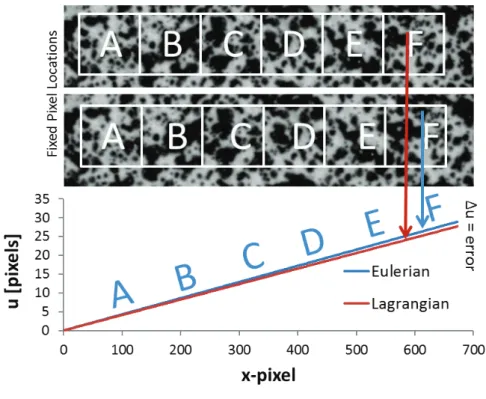
The error associated with the Eulerian and Lagrangian frames can be a difficult idea to explain and illustrate, but we try to do so here. First, two concepts: DIC is inherently Lagrangian in that it tracks the subset from the reference location in the reference image to its new location in the deformed image. The subset is the boat floating down the river in the famous example. Second, simulations are naturally Eulerian. That is, the speckles (effectively intensities or grey values in the image) are moved to a new position by applying the desired displacement field to the image intensity values. The intensity values at the fixed pixels in the deformed image are then calculated from the shifted speckle pattern. The pixels are like standing on the bridge looking down on the speckle field floating underneath. We illustrate the difference between Lagrangian and Eulerian description of motion in Figure 8, which shows a speckle pattern that was shifted by a linear, horizontal stretch. The speckles associated with region “F” are moved to the new location by applying the deformation field (blue line). The rectangles correspond to pixels
(as this is an illustration ignore that the pattern is too small), and the new grey values are calculated at these fixed pixel locations as the speckle field translates under the pixels. This makes the simulation inherently Eulerian.
Figure 8. Illustration of the Lagrangian versus Eulerian problem.
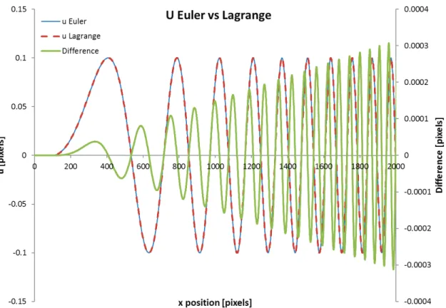
There are two possible fixes to the results. The first involves using the function used to create the displacement and strain field, and finding the displacement value at the correct Lagrangian location (XL and YL), found by getting the displacement at XL = (XE – u(XE)) or YL = (YE – v(XE)); where XE and YE represent the integer pixel locations in the reference Eulerian state and u(XE) and v(YE) the commanded displacements from that reference state. Note that these coordinates will be at a non-integer subpixel positions, whereas the commanded u and v values calculated were at reference integer pixel locations in the Eulerian coordinates. We used a second solution that involves interpolating the command position to find the correct value in the Lagrange coordinates for comparison with DIC. The same equations are used to find the XL and YL locations at which the commanded displacement field is then interpolated. A cubic spline interpolant was used for Sample 14 and a Hermite polynomial (pchip in MatLAB and an equivalent LabVIEW function) was used for Sample 15 as it deals with the discontinuity better. Figure 9 shows the effect of this error on the results for a 1D cut through the data in the middle of the image of Sample 14. Note that looking at the curves for uE versus uL it is not possible to tell the difference between the two results, and indeed for these curves the error between the two coordinate systems is less than 3 1000⁄ 𝑡𝑡ℎ of a pixel.
This is well below experimental errors; however, synthetic images must be correct! Errors in Sample 15 were similar but of larger magnitude because of the larger displacements involved.
Figure 9. Illustration of the Euler versus Lagrange error using Sample 14. Blue curve is the commanded displacement field, red curve is the corrected Lagrange displacement field (aka the DIC results) and the green curve is the difference. Note the growing error as it accumulates across the image.
5.4 Sample analysis procedure
5.4.1 Analysis Software
The analysis presented in this paper was done using National Instruments LabVIEW software (v2015), and the results were verified using MatLAB code written by a second person. The executable files and source-code for both the LabVIEW and MatLAB analysis codes are available for download at the DIC Challenge website. DIC researchers are encouraged to make use of these codes as suitable in publications claiming 2D-DIC accuracy improvements, and DIC users are encouraged to use these codes to understand the “black box” that is most commercial DIC software. A standard set of algorithms, used by all authors, makes comparisons of different DIC algorithms and software packages more straightforward and efficient.
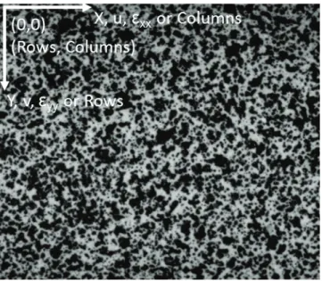
The analysis code uses standard array definitions of the image processing community with index (0,0) defined as the top-left corner of the image, and rows and columns defined as in Figure 10. Standard computer numbering for arrays is also used, with numbering starting at 0 rather than 1. Note: some of the submissions were off by one
pixel and were shifted accordingly. The directions for the displacements and strains are also defined in Figure 10 using standard DIC notation.
Figure 10. Coordinate system definition for the analysis codes. We use the standard “Image” definition for arrays, with 0,0 at the top-left corner of the array.
5.4.2 Submission Guidelines
The results were submitted using a comma separated value file (*.csv). We created the LabVIEW and MatLAB code with the flexibility to deal with the inevitable differences in the file format between the US, Europe and Asia. Separators in the file can include either commas (US), semicolons (Europe), or tabs. Flexibility was also incorporated in the code to define the decimal delimiter as either a period (US) or a comma (Europe). Participants reported the results with a 5-pixel step size in both the rows and columns. Global results reported the value at the center of the pixel to match the results of the subsets. Note that any errors of a possible ½-pixel discrepancy due to these definitions should be small relative to the other errors encountered. The 5-pixel step size in result reporting, however, led to significant difficulties in precise analysis as data interpolation between the reported values was required. We describe this interpolation in detail in the results section. Future results will be submitted with a 1-pixel step in the results to simplify and improve the analysis.
Both Sample 14 and Sample 15 were 1D displacement fields imposed on 2D images. Therefore, each row in Sample 14 and column in Sample 15 have the same displacement and strain. This data redundancy was used to probe the bias and noise errors of DIC by averaging along either the rows or columns. Doing this yields a mean value, which provides a cleaner visualization of the bias errors. Bias errors for the synthetic images indicates an offset from the known value and is caused by spatial filtering of the DIC algorithms, by the subset size and shape function, and by the virtual strain gage used to calculate the strain. The standard deviation at each point along the row or column indicates the noise. All plots and figures unless otherwise stated use 1-standard deviation (1σ) for the reported noise value.
5.4.4 Root Mean Square Error
Another approach used to summarize the error of the full-field results in a single number is the Root-Mean Square Error (RMSE). Bornert [28] introduced this concept in his DIC uncertainty paper. The following equations define the RMSE for the displacement u (or v), and similarly, but not shown, for the strain εxx (or εyy).
𝑅𝑅𝑅𝑅𝑅𝑅𝑅𝑅 = �𝑛𝑛1∑ [∆𝑢𝑢]𝑖𝑖,𝑗𝑗 2 Equation 2
∆𝑢𝑢 = 𝑢𝑢𝑖𝑖,𝑗𝑗𝐶𝐶𝐶𝐶𝐶𝐶𝐶𝐶𝐶𝐶𝑛𝑛𝐶𝐶𝐶𝐶𝐶𝐶− 𝑢𝑢𝑖𝑖,𝑗𝑗𝐷𝐷𝐷𝐷𝐶𝐶 Equation 3
where i,j represent the row and column pixel locations and n is the total number of reported DIC data points. Because subset-based codes do not provide data at the image perimeter (and because the size of this region without data varies for different DIC codes), we calculated the RMSE for Sample 14 only in the interior region from pixel (50,50) to (545,1995) in an image size of 588 × 2048 for 39,000 data points. Similarly, for Sample 15, we used the interior region of (50,50) to (945,1930) in an image size of 1000 × 2000 for 67,304 data points.
5.4.5 Spatial Resolution Measurement
DIC can be thought of as a nonlinear low pass filter in the spatial domain. The cut-off frequency and roll-off of the filter are determined by the characteristics of the DIC code, including user-selectable quantities such as subset size, step size, virtual strain gage size, and other nonuser-selectable quantities such as the interpolant, subset shape function, strain calculation methods, and any filtering hidden from the user. DIC filtering is unavoidable but also
often needed to reduce experimental noise. DIC users, therefore, need a method of understanding and representing DIC filtering, and how filtering adds bias error to DIC results and changes spatial resolution.
One possible method for quantifying spatial resolution, adopted by the DIC Challenge, is to measure the ability of a code (given a set of user-selected settings) to capture the peak displacement or strain in the sinusoidally-varying deformation field of Sample 14. Depending on the amount of filtering of the DIC results, the amplitude of the peak will be captured well at low frequencies, but will be attenuated at higher frequencies. The cut-off frequency is the point at which attenuation begins, and the roll-off is the rate of attenuation after the cut-off frequency (using standard filter terminology). The spatial resolution is then defined as the inverse of the cut-off frequency with pixels as the units. These two quantities provide metrics for comparing the filtering effects of different DIC codes and the effects of different user-selected settings, and serve as a standard basis for understanding and presenting the spatial resolution of DIC results.
5.5 DIC Challenge results
5.5.1 Sample 14
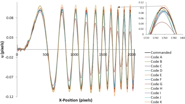
The spatially varying displacement and strain value of Sample 14 provided in a single image the opportunity to measure both the noise level (the first columns in the left portion of the image have no displacement field) and the spatial filtering of the DIC codes with the increasing frequency displacement field in the right portion of the image. Most of the codes captured even the highest gradients in these images. Future studies from the challenge will include similar images, but with both higher displacements and higher frequencies in the displacement field to better challenge all the codes. Even with that drawback, the images provide a context for discussion on how to quantify spatial resolution in DIC measurements. (The full-field contour plots of the horizontal displacement from Codes A through K are shown in Appendix B, Figure 35). These contours give a visual sense of the displacement noise versus smoothing in the analysis. Some filtering can also be seen, particularly in Code A. Another way of visualizing the results is by taking a horizontal line-cut and averaging 50-rows as discussed previously. Those results are shown in Figure 11 and also illustrate the spatial filtering in a variety of the codes.
Figure 11. Line cut results showing the mean of the reported values, the commanded displacement, the bias error and the noise. The inset highlights reductions in peak amplitude caused by spatial filtering.
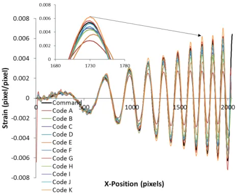
The full-field contour plots of the horizontal strain field are presented in Appendix B Figure 36, while the horizontal line cuts (averaged over 50 rows) are presented in Appendix B Figure 37. Strain fields always have more spatial filtering than displacement fields for two reasons. First, some number of displacement values spanning a region in space are required to compute the displacement gradients. The region of displacement data used in the strain calculations is referred to as the “virtual strain gage”, and the calculated strain is the average strain in this area. Note that this same effect is seen with traditional strain gages, where the physical size of the gage averages the strain field beneath it. The virtual strain gage effect is seen regardless of the method of calculating strain, whether this is fitting a curve to a region of displacement data to get the derivative, or using neighboring points in an FE type strain calculation and then averaging, or any other process. Second, the derivative amplifies small amounts of noise in the displacement field in the resulting strain field. Therefore, a larger virtual strain gage is often required to reduce the noise in the calculated strains, which increases the spatial filtering of the strain field.
Figure 12. Line cut results showing the mean of the reported values, the commanded strain.
For Sample 14, 50 rows were averaged together and the mean and standard deviation were calculated at each reported step (that is every 5-pixels) along the columns. To compute the bias error, the measured mean displacement field was subtracted from the commanded value. The commanded value, mean measured value, bias and standard deviation curves for select codes are shown in Appendix B Figure 37. Table 4 lists the average noise for both the displacement and strain for all columns.
Table 4. Average standard deviation as a measure of overall result noise for Sample 14 L5.
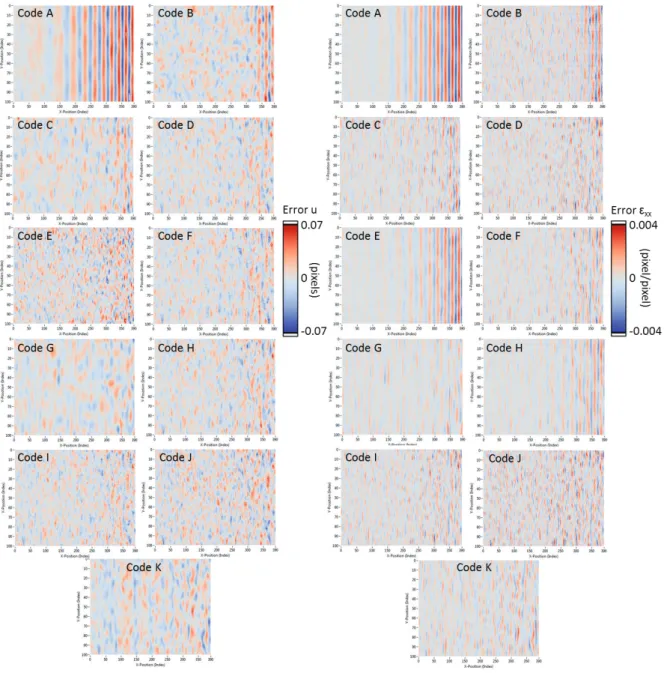
To better understand results, it is also useful to visualize the full-field errors and summarize them numerically. The error plotted in Figure 13 is the difference between the commanded (displacement or strain) and the measured value (Equation 3). The results in Figure 13 clearly illustrate the trade-off in filtering and bias error. Vertical noise
is clearly seen in the full-field results and is common to all codes. The width of the banding is related to the amount of filtering. Table 5 summarizes the results using the root-mean-square error (RMSE) as defined in Equation 4. The RMSE provides an overall quality measurement by combining both the noise and the bias errors into a single metric. Also listed in the table is the absolute maximum error. This indicates the largest deviation of the measured DIC result from the commanded displacement or strain field.
Figure 13. Full-field error plots for all the codes for both displacement (left) and strain (right). All scales are identical and the results are plotted in standard image array format to match the image deformation field.
Table 5. Root-mean-square error (RMSE) and absolute maximum bias error.
5.5.2 Determining spatial resolution from bias analysis
In this investigation, the spatial resolution was defined as the ability of the DIC results to recreate a displacement or strain field that has a spatially varying frequency. The DIC challenge designed Sample 14 to have a 1D swept sine with constant amplitude and increasing frequency (Figure 6). The low-pass filter effect of DIC is reflected most intuitively in the roll-off of Sample 14 L5. The “roll-off” of the filter is visualized by calculating the signal attenuation as a percent of the command value as (peak or valley)/(command value). The commanded displacement peaks or valleys were set to ±0.1 pixels throughout the image. A LabVIEW peak detection algorithm found the peaks on both the commanded and measured displacement and strain values. The peak detection fits a quadratic function to a small region of data points to find the peak or valley location. We calculated the spatial frequency by finding the distance in pixels between neighboring peaks and valleys in the signal, both the peaks and valleys were used to have twice the number of data points across the image. The spatial period was then calculated as 2× the distance between any neighboring peaks or valleys. The percent of commanded value is plotted for the displacement as shown in Figure 14 (strain was also calculated but not shown). A 3rd order
polynomial was then fit to find the cut-off frequency. The curve was used to find the crossing point of the roll-off of either 95% or 90% of the commanded value for the displacement and strain respectively. This represents a 5% bias error in the displacement and a 10% bias error in the strain. These values were chosen as reasonable, although arbitrary. Regardless of the levels chosen, all codes were analyzed in the same way.
Note that we have purposely chosen to treat the calculation of the spatial resolution with a “black box” approach, rather than calculating the transfer function as has been done in previous work [29,6,30]. This was done because of the multiple implementations of DIC that are analyzed in this work, including local DIC, global DIC, adaptive
DIC, and other implementations of a proprietary nature. The advantage of this approach is that using simple techniques with synthetic images, the spatial resolution can be estimated for any arbitrary implementation.
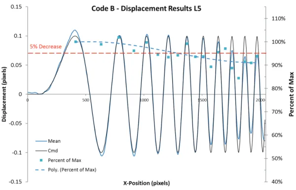
Figure 14. Displacement results for Code B for Sample 14 L5. Shows the command, mean, bias, standard deviation and percent of maximum. 3rd order
polynomial fit and 95% value shown to illustrate how the cut-off frequency was chosen.
Table 6 contains the cutoff frequencies found using the LabVIEW analysis code. The table includes the standard deviation from Table 4 to communicate an important point: All codes trade between the spatial resolution and the noise. We required the participants to choose only one data set to submit, which entails a compromise in the analysis. Different participants chose different compromises between smoothing and bias. For example, Code A has the lowest noise by a factor of at least 2, but also has the worst spatial resolution; on the other hand, Code E and Code J have the highest noise but nearly the best spatial resolution. Code K overestimates the displacement and strain without roll-off for these images. Most of the other codes seemed to choose about the same compromise and have nearly identical cut-off frequencies and noise levels. However, with the given requirements, it seems that Code G scores the best in this evaluation.
Table 6. Cut-off frequencies (and spatial resolution) for both displacement and strain
5.5.3 Sample 15
Sample 15 has eight cases that could be analyzed with an increasing strain gradient on one side of a concentration and a step response to zero strain on the other side as pictured in Figure 7. We have chosen to analyze image “P200_K250.tif” for this paper as it has nicely separated peaks with a large strain value. The other images are similar with the peaks moving closer together (K50) or farther apart (K400) and with small changes in the maximum strain amplitude. For K250, the maximum strain is in the Y-direction (εyy) and has a peak strain of 0.054
pixel/pixel or 54000 με. The spatial resolution analysis conducted for Sample 14 does not apply to Sample 15; instead, we will focus on the bias errors, RMSE, and maximum acceptable bias error metric.
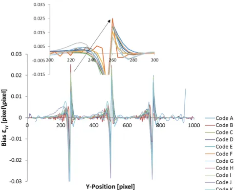
Consistent with Sample 14, the columns of Sample 15 were averaged across the image using a total of 188 columns to create the average (this is every other column). Sample 15 has more rows than Sample 14 because the image was wider (there was no important difference caused by this). The mean value was then subtracted from the commanded to yield the bias error as plotted in Figure 15. Table 7 contains the calculated average standard deviation for the line cut and the maximum absolute value of the bias error.
Figure 15. Bias error for Sample 15 K250 for all codes. This is the mean of 188 columns subtracted from the command value. Note the large error at the discontinuity.
Table 7. Average standard deviation and absolute maximum bias error from the line cuts. Data corresponds to the line cuts in Figure 15.
The full-field difference plots are shown in Figure 16 for both the displacement and strain. The range of the color bar is set to be ±5% of the full-scale commanded displacements and ±10% of the full-scale commanded strains. While there are some differences in how the codes handle the noise and the discontinuity, the basic features were similar for all codes. Namely, some displacement and strain data is outside the predetermined range near the discontinuity, with larger errors on either side of the discontinuity (except for Code B, which had random noise distribution spatially). Table 8 presents the RSME, the maximum bias, and the percent of reported points that were within the predetermined range. This table again illustrates the tradeoff between filtering and bias errors.
Code B for example does a better job of capturing the peak displacement (low maximum bias) but has more noise throughout the image. Other codes, such as Code G, have much lower noise throughout the field, but still miss some region of the peak strain and displacement.
Figure 16. Full-field error plots for the displacement (left) and strain (right). Difference between commanded and DIC results. The scales represent ±0.5% of full-scale for displacement and ±10% full-scale for strain. These correspond to the limits in Table 8. White regions in the data field are points either above or below the plot ranges, rather than missing data.
Table 8. RMSE error for both displacement and strain for the full-field data shown in Figure 16.
6. Conclusions
It is human nature to compete – and therefore a “score” seems necessary. However, scoring is not the primary purpose of the DIC Challenge, and the challenge board did not rank the codes from 1 to N. We seek to provide a methodology and defined metrics to assess DIC codes that will be used in future publications. The development of thought on how to quantify spatial resolution is a good example of this progress. However, we think presenting the performance relative to several different metrics will allow a view of how well a code is performing for a given application. The following list of goals is more important for the challenge board than a score.
1. A verified and validated set of images (and corresponding displacement fields) for people to use in publications and code development. The errors already discovered regarding Eulerian versus Lagrangian coordinate systems are an illustration of the importance of this!
2. An understanding of the compromise in DIC code between filtering and noise, also known as the regularization length.
3. Motivation for improvements in DIC codes where necessary, particularly for university codes. 4. Defined metrics that have a broad community consensus on how to quantify a “good” DIC result. 5. A formation of a consistent vocabulary (e.g., “spatial resolution”). See a recent paper by Grédiac that
discusses this in detail [30].
The preliminary sample DIC challenge image sets and analysis were an important first step in helping the DIC community to better understand what influences the quality of their DIC results. All the image sets provide a basis for evaluating the DIC software with different sets providing different challenges to the DIC algorithm; noise robustness, lack of contrast, interpolation errors and so forth. These images can be used for software verification. Verification is defined as testing the code to see if it is functioning correctly. The images cannot be used for experimental validation. That is, these images will not quantify the expected uncertainty in an experiment. Many of the error sources are missing in the synthetic images, which only include image noise, and therefore are not relevant for determining experimental error bounds. Rather, the challenge images would be the “best case scenario” in an experiment for a given speckle pattern and image noise. Remember the images analyzed for the challenge (Sample 14 and Sample 15) are synthetic images! The errors determined here may be only a small portion of the error budget for many experiments. Anything less than 1/100th of a pixel of error is likely not going
to be seen in an actual physical experiment. On the other hand, the experimental image sets do include all the errors that occur, but either do not have known results or are simplistic in their displacement fields (e.g., rigid body displacement).
Scoring of the codes in this paper is incomplete. Some have said that for a typical analysis, the experimentalist would optimize the DIC software settings with an often better defined goal in using the results. This can often be done with a virtual strain gage size study varying the parameters to investigate the filtering effect, balanced against the need to contain noise. In fact, this is how one should typically conduct their post processing. However, it is the balance between the noise and bias that is difficult to determine. In defense of the approach the board has taken, let us note that in most analysis, you probably want both great spatial resolution and minimized noise! We do not think that the task set for the analysis of these images is substantively different than for a typical experiment: You have a set of images and want to get the best results possible. Even if you are going to use this to calculate material properties as an integrated step, the balance of noise and bias will be an important and maybe poorly understood compromise.
We cannot emphasize enough the goal of this exercise was not to rank the codes – but provide a forum for understanding how DIC is working. We think that it is generally true that given different solution parameters, each of the 10 codes could be brought to be even closer to each other in performance. That is, the quality of the results for 2D-DIC depend more on the selection of the DIC software analysis settings than it does on the implementation of the code (at least for those participating in this challenge). Therefore, training is an important component in adopting DIC as a primary measurement technique in the lab. It is easy to get answers from DIC, it
is harder to always get good answers from DIC. It should also be emphasized that for many experiments the quality of the results is driven far more by issues with the experiment – than issues with the DIC code. Out-of-plane errors [31] and heat waves [32] are just two examples that will most often overwhelm the errors within the DIC implementation.
It is hoped that all future publications would use DIC Challenge image sets when making claims of improvement in the quality of the results. Without a common set of images, there is no meaningful method of comparison. Note that both the images used and the software required to analyze the images are freely available on the SEM website. As reviewers, we should be insisting on the use of these images in order to be able to draw meaningful conclusions from papers on 2D-DIC accuracy.
7. Future Goals of the DIC Challenge
After the publication of this paper, a final round of images will be provided that are blind. These blind images will be based on Sample 14 and Sample 15 (see Table 1), but with deformation fields unknown to the participants. These images will be provided to all who desire to participate, with the results to be published in a subsequent paper. The advantage of blind image sets is that any possibility of impropriety is removed from the analysis portion by the participants. Additionally, standard image sets for stereo-DIC are currently being designed, and the 2D-DIC Challenge will be extended to stereo-2D-DIC. Preliminary image sets, including both calibration images and deformed images, are at the Challenge website. There will be both synthetic images created using the Balcaen simulator and completely experimental image sets. The experimental image sets will be used for round-robin code comparison and for measurements against secondary diagnostics. The Challenge Board invites your comments and ideas.
3. Acknowledgements
The 2D-DIC Challenge is dedicated to Dr. Laurent Robert. An active and important board member in the early years of the project, who passed away in 2016. He has been sorely missed in the experimental mechanics community. The Challenge would like to thank, Francois Hild, Stephane Roux and Bernd Wieneke for pointing out the Lagrange/Euler discrepancy and suggesting solutions to that problem.
Sandia is a multiprogram laboratory operated by Sandia Corporation, a Lockheed Martin Company, for the United States Department of Energy’s National Nuclear Security Administration under contract No.