HAL Id: hal-03127329
https://hal.archives-ouvertes.fr/hal-03127329
Submitted on 1 Feb 2021
HAL is a multi-disciplinary open access
archive for the deposit and dissemination of
sci-entific research documents, whether they are
pub-lished or not. The documents may come from
teaching and research institutions in France or
abroad, or from public or private research centers.
L’archive ouverte pluridisciplinaire HAL, est
destinée au dépôt et à la diffusion de documents
scientifiques de niveau recherche, publiés ou non,
émanant des établissements d’enseignement et de
recherche français ou étrangers, des laboratoires
publics ou privés.
A generic approach for efficient detection of vascular
structures
Amele Florence Kouvahe, Catalin Fetita
To cite this version:
Amele Florence Kouvahe, Catalin Fetita. A generic approach for efficient detection of vascular
struc-tures. Innovation and Research in BioMedical engineering, Elsevier Masson, 2020, 41 (6), pp.304-315.
�10.1016/j.irbm.2020.06.011�. �hal-03127329�
A generic approach for efficient detection of vascular structures
Amele Florence Kouvahé
and Catalin Fetita
SAMOVAR, TELECOM SudParis, Institut Polytechnique de Paris, France
ABSTRACT
Vascular segmentation is often required in medical image analysis for various imaging modalities. Despite the rich literature in the field, the proposed methods need most of the time adaptation to the particular investigation and may sometimes lack the desired accuracy in terms of true positive and false positive detection rate. This paper proposes a general method for vascular segmentation based on locally connected filtering applied in a multiresolution scheme. The filtering scheme performs progressive detection and removal of the vessels from the image relief at each resolution level, by combining directional 2D-3D locally connected filters (LCF). An important property of the LCF is that it preserves (positive contrasted) structures in the image if they are topologically connected with other similar structures in their local environment. Vessels, which appear as curvilinear structures, can be filtered out by an appropriate LCF set-up which will minimally affect sheet-like structures. The implementation in a multiresolution framework allows dealing with different vessel sizes. The outcome of the proposed approach is illustrated on several image modalities including lung, liver and coronary arteries. It is shown that besides preserving high accuracy in detecting small vessels, the proposed technique is less sensitive with respect to noise and the presence of pathologies of positive-contrast appearance on the images. The detection accuracy is compared with a previously developed approach on the 20 patient database from the VESSEL12 challenge.
Keywords: locally connected filters, vascular detection, mathematical morphology
1. Introduction
Vascular segmentation is required in several applications: diagnostic assistance, interventional support in surgery or vascular disease monitoring. The difficulty of efficient detection and segmentation of vascular structures is related to the great variability of vessel appearance on images according to the clinical modality and acquisition protocol. Vessels show up as curvilinear structures of positive (or negative) contrast with respect to their environment. They may present various subdivision degrees over several scales of diameters, sometimes going beyond the image resolution limit. At the image level, their diameters extend from one to several tens of pixels (voxels). Note also that the normal “tubular” shape at a given scale may be distorted by the presence of noise or pathology (inducing vascular remodeling).
The detection of vessels as curvilinear structures may be tackled from two points of view: (i) denoising / filtering and (ii) enhancement / segmentation. Filtering involves reducing the noise level in an image while preserving the structures of interest. The segmentation consists in detecting these structures with respect to the rest of the image, for example with a result presented in the form of a binary image.
Several literature reviews for vascular segmentation can be found [1 – 6]. The first ones [1] [2] focus on the segmentation of vessels in images obtained by MRA (Magnetic Resonance Angiography). It is divided into two parts: a first dedicated to prefiltering [1], and a second that compares skeletal extraction methods with those that detect the entire vascular volume [2]. The second study [3] more generally concerns the segmentation of vessels from all types of images, regardless of their size or acquisition modality. The third review [4] investigates the images obtained by MRA and CTA (Computed Tomography Angiography) and lists the methods according to three axes: (i) vascular models, i.e. information on the targeted vessels, (ii) the vessel-specific characteristics, i.e. the measurements used to detect the vessels, and (iii) the extraction schemes, i.e. the algorithms used for the segmentation of the vessels.
The fourth study [5] also applies to images from MRA and CTA, but class the methods into eight families: region growing [7], segmentation based on models [8], deformable models [9], path research [10], vessel tracking [11], mathematical morphology [12], statistical approaches [13] and filtering based on derivatives [14]. The first six families are segmentation methods; statistical approaches can be used for both segmentation and filtering, and the last family is typically a filtering method. The most recent studies [6] focus on the latest innovations, in particular in machine learning, deformable models and tracking-based approaches. They
distinguish the following categories: supervised [15] or unsupervised [16] learning, deformable models based on contours [17] or based on regions [18], monitoring methods [19]. Each of the methods is applied to one or two
regions, excepting one, based on active contours, which has been used for several regions: abdomen, brain, heart, lungs and retina [18].
However, despite steady progress and efforts in the field, several issues still need to be solved. A relevant limitation is the segmentation of pathological vessels. Additional research is needed because some of the main assumptions about healthy vessels (such as linearity and circular cross section) are not valid in pathological conditions, which require new vessel model formulations. It can be said that to date, no single segmentation approach is suitable for all anatomical regions or different imaging modalities.
This article proposes a new method for detecting and segmenting vascular (and curvilinear) structures, which use locally connected filtering applied in a multiresolution scheme. The method is general and exploits the property of appearance (positive contrast) and the geometry of the vessels. The approach can also be used for structures in negative contrast, either by working on the complement of the image, or by using a suitable operator (cf §2). The result of the proposed approach is demonstrated on images of different modalities and on vessels of different organs (lungs, liver and heart).
2. Materials and Method
The central idea of the proposed method is to distinguish curvilinear structures with positive contrast from other structures of similar intensity but of different geometric shapes. The method relies on locally connected filtering applied in a multiresolution scheme to remove curvilinear structures in native images. These structures (vessels) are then reconstructed from the difference with the original data.
In the following section, we introduce the mathematical principle of locally connected filters that will be used for vascular detection. In section 2.2 we show how applying these filters with respect to various oriented reference sets will result in suppressing vascular structures from images while preserving other positive contrast elements of non-curvilinear shape. We illustrate an example of application in the 2D case (§2.2.1) and in the 3D case (§2.2.2), before summarizing the multiscale approach proposed for 3D vascular segmentation in section 2.2.3.
2.1 Locally connected filters for vascular detection
Let f: 𝑉 ℤ𝑛→ ℤ a discrete compact support function. We define the topological graph G associated with
f
asthe tuple G(V, E), where E denotes the set of edges 𝑒 = 𝑥, 𝑦 connecting two distinct elements (nodes) of V, x, y ϵ V . The construction of the graph G is determined here by the adjacency relationship considered between the elements of V for the definition of the E set. For example, in ℤ2, G can be defined by 4- or 8-connectivity, and in
ℤ3by the 6-, 18- or 26-connectivity.
Without loss of generality, we will illustrate the following different concepts on regular graphs defined on ℤ2 or
ℤ3 by the abovementioned adjacency relationship.
Let f: 𝑉 ℤ𝑛→ ℤa discrete compact support function and G(V,E) the topological graph associated with V. Two
elements (graph vertices) of V, x,y ϵ V are adjacent x ≈ y iff there is an edge 𝑒 = 𝑥, 𝑦 ϵ E on G linking x and y (Fig. 1).
A path between any two points on G, 𝛤(𝑥,𝑦)𝐺 G is defined as the subset of adjacent vertices {zi}i ϵ V and edges
{𝑒𝑖𝑗 = 𝑧̅̅̅̅̅̅} 𝜖 𝐸, allowing to connect x and y such that x= z𝑖, 𝑧𝑗 1, z1≈ z2, …, zn-1≈ zn, zn =y:
𝛤𝑓𝐺(𝑥, 𝑦) = {{𝑧𝑖 }𝑖 𝜖 𝑉 ∪ {𝑒𝑖𝑗= 𝑧̅̅̅̅̅̅}𝑖 , 𝑧𝑗 𝜖 𝐸|𝑥 = 𝑧1, 𝑧1≈ 𝑧2, … , 𝑧𝑖≈ 𝑧𝑖+1, … , 𝑧𝑛 = 𝑦 }. (𝟏)
Fig.2 illustrates some examples of paths on two types of graphs in ℤ2
.
(a) 4-connectivity adjacency (b) 8-connectivity adjacency
(a) (b)
Fig. 2. Example of paths 𝛤𝑓𝐺 between two points x and y on a graph G (V, E), V ℤ2, defined by (a) the
4-connectivity and (b) the 8-4-connectivity adjacency relationship.
We define the maximum / minimum altitude on the relief of f along a path 𝛤𝑓𝐺 as ;
𝑆𝑢𝑝𝛤𝑓𝐺(x, y) = 𝑠𝑢𝑝{𝑓(𝑧)| ∀𝑧 𝛤𝑓𝐺(𝑥, 𝑦) } , (𝟐)
𝐼𝑛𝑓𝛤𝑓𝐺(𝑥, 𝑦) = 𝑖𝑛𝑓{𝑓(𝑧)| ∀𝑧 𝛤𝑓𝐺(𝑥, 𝑦) } , (𝟑)
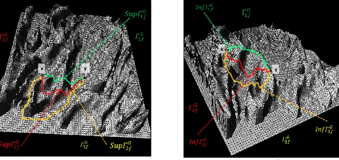
where G denotes the topological graph G(V, E) associated with f, inf – the infimum and sup – the supremum. Figure 3 illustrates an example of 𝑆𝑢𝑝𝛤𝑓𝐺and 𝐼𝑛𝑓𝛤
𝑓𝐺for a function f :𝑉 ℤ𝑛→ ℤ along different paths 𝛤𝑓𝐺.
We define the sup-connectivity CT (respectively the inf-connectivity, CT) between two points x, y ϵ V on the relief of a function f :𝑉 ℤ𝑛→ ℤ as being the highest (respectively the lowest) minimum (respectively
maximum) altitude of the relief of f along all the possible paths connecting x and y on the graph of f (Figure 4):
𝐶𝑇𝑓𝐺(𝑥, 𝑦) = 𝑠𝑢𝑝{𝐼𝑛𝑓𝛤𝑓𝐺(𝑥, 𝑦), 𝛤𝑓𝐺(𝑥, 𝑦)},
(𝟒)
𝐶𝑇𝑓𝐺(𝑥, 𝑦) = 𝑖𝑛𝑓{𝑆𝑢𝑝𝛤
𝑓𝐺(𝑥, 𝑦), 𝛤𝑓𝐺(𝑥, 𝑦)},
where G denotes the topological graph G = (V, E) associated with f.
(a) (b)
Fig. 3. Illustration of the value of 𝑆𝑢𝑝𝛤𝑓𝐺 (a) and 𝐼𝑛𝑓𝛤
𝑓𝐺 (b) on different paths 𝛤𝑓𝐺 connecting two points x and y on a graph G (V, E). f is represented as a mesh surface.
(a) (b)
Fig. 4. Sup and Inf-connectivity: illustration of the value CT (a) and CT (b) between two points x and y on a graph
G(V, E) and the corresponding path (not necessarily unique). Note that in (a) CT(x,y) = sup (f(x),f(y)) while in (b) CT(x,y) = inf (f(x),f(y)), not shown on these images.
We similarly introduce the concepts of topological sup/inf-connectivity between a point x ϵ V and a subset Y V based on the extension of the definition of the path between a point and a subset of the graph nodes.
Let f: 𝑉 ℤ𝑛→ ℤa discrete compact support function and G the topological graph G(V,E) associated with f. Let
Y V be a reference subset. We define the connection path between a point x ϵ V and Y as the set of paths connecting x and any point y of Y:
𝛤𝑓𝐺(𝑥, 𝑌) = {
{𝛤𝑓𝐺(𝑥, 𝑦)}
𝑦 𝜖 𝑌 , 𝑖𝑓 𝑥 ∉ 𝑌
𝑥, 𝑜𝑡ℎ𝑒𝑟𝑤𝑖𝑠𝑒.
(𝟓)
The set of minimum / maximum altitude along the paths connecting a point x ϵ V and a subset Y V is then similarly defined as:
𝐼𝑛𝑓𝛤𝑓𝐺(𝑥, 𝑌) = {𝐼𝑛𝑓𝛤𝑓𝐺(𝑥, 𝑦)}𝑦 𝜖 𝑌 , (𝟔)
𝑆𝑢𝑝𝛤𝑓𝐺(𝑥, 𝑌) = {𝑆𝑢𝑝𝛤𝑓𝐺(𝑥, 𝑦)}𝑦 𝜖 𝑌 .
The sup-connectivity (respectively the inf-connectivity) between a point x ϵ V and a set Y V are defined by
𝐶𝑇𝑓𝐺(𝑥, 𝑌) = 𝑠𝑢𝑝{𝐼𝑛𝑓𝛤𝑓𝐺(𝑥, 𝑌)} = 𝑠𝑢𝑝(𝐶𝑇𝑓𝐺(𝑥, 𝑦)), ∀ 𝑦 𝜖 𝑌, (𝟕)
𝐶𝑇𝑓𝐺(𝑥, 𝑌) = 𝑖𝑛𝑓{𝑆𝑢𝑝𝛤𝑓𝐺(𝑥, 𝑌)} = 𝑖𝑛𝑓(𝐶𝑇𝑓𝐺(𝑥, 𝑦)), ∀ 𝑦 𝜖 𝑌.
𝐶𝑇𝑓𝐺(𝑥, 𝑌) represents the lowest altitude at which we have to descend on the relief of f by seeking to connect x
and Y on G while favoring the high altitude paths (the passes).
𝐶𝑇𝑓𝐺(𝑥, 𝑌) represents the highest level to cross on the relief of f by seeking to connect x and Y on G while
privileging the low-altitude paths (the ravines).
(a) (b)
Fig. 5. Illustration of the sup-connectivity (a) and the inf-connectivity (b) between a point x and a subset Y on the topological graph G associated with the function f. Note that (a) corresponds to the path that retains the highest altitudes
and (b) the path that retains the lowest altitudes by connecting x to Y on the relief of f.
Note that, from an algorithmic point of view, in the case where the topological graph G associated with f is defined in the space ℤ𝑛 based on the adjacency relationship given by spatial connectivity (4-c, 8-c in 2D , 6-c, 18-c or
26-c in 3D), the two operators
𝐶𝑇
𝑓𝐺(𝑥, 𝑌)
and𝐶𝑇
𝑓𝐺(𝑥, 𝑌)
can be computed using the morphological operators of numerical reconstruction by dilation Rf(x,Y) for CT, or numerical reconstruction by erosion Rf(x,Y) [20] forCT. We can speak in this case of the reconstruction of the topological connectivity between x and the set Y.
2.2 Segmentation of vascular structures by locally connected filters
Concerning the application envisaged for the vascular segmentation and taking into account that the vessels present a positive contrast in the selected modality (computed tomography), we will subsequently exploit the sup-connectivity operator CT defined above.
If we consider two points x, y inside the 3D vascular structure, the value 𝐶𝑇𝑓𝐺(𝑥, 𝑦) will be high because of the
presence of a high intensity path connecting x and y along the axis of the vessels. Similarly, when the vascular structure is immersed in a network of fibrosis reticulations, also of high intensity, the value
𝐶𝑇𝑓𝐺(𝑥, 𝑦) computed between a point x inside the vessels and a point y inside the surrounding reticulations will
also be high (due to the high intensity connection between vessels and reticulations) which does not allow to discriminate the two anatomo-pathological structures using CT.
To achieve this, we will study a directional procedure which uses CT in a 2D context, according to oriented section plans. We start from the observation that, in a plane orthogonal to the axis of the vessel, the vascular section will be disconnected from its neighborhood Y (that is, 𝐶𝑇𝑓𝐺(𝑥, 𝑌) will be small for all x in the vessel
section). On the other hand, because of their honeycomb geometry, the reticulations keep a connection with their neighborhood, regardless of the section plane, which provides a means of differentiation with the vessels. In conclusion, unlike literature methods that attempted to select vessels by analyzing contours along the central axis of structures [21][22], we chose to implement a directional local filter, which uses CT, in order to
differentially remove the vascular structures in the images, to finally segment them by difference with the native data.
Let f: 𝑉 ℤ𝑛→ ℤa discrete compact support function and G the topological graph G(V,E) associated with f.
We define the locally connected filter by dilation LCFf,k(x) of size k at the point x ϵ V:
LCFf,k(x)= 𝐶𝑇𝑓𝐺(𝑥, 𝑁𝑘(𝑥)), (𝟖)
with 𝑁𝑘(𝑥) = {𝑦 𝜖 𝑉|𝑑(𝑥, 𝑦) > 𝑘}, (𝟗)
LCFf,k reconstructs locally the 𝑓 value from a k-distant neighborhood by grayscale morphological dilation. Its
effect is to attenuate (or suppress) the f values which are not “linked” with their k-distant neighborhood via a high-intensity path. On contrary, when such connection exists, the structures are preserved via the reconstruction operator with a slight “flattening” of the grayscale levels.
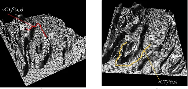
Figure 6 illustrates the effect of LCFf,k filtering at the central point of a region of interest (ROI) for two image
configurations, where the neighborhood 𝑁𝑘 is chosen as in eq. 9, with a distance function d8 given by:
𝑑8(𝑎, 𝑏) = max(|𝑎1− 𝑏1|, |𝑎2− 𝑏2|), (𝟏𝟎)
where 𝑎𝑖,𝑏𝑖denote the 2D coordinates of points a and b. This example is a typical case of differentiation
between points in vascular structures (Fig. 6a) and points in fibrosis reticulations (Fig. 6c).
(a) (b) (c) (d)
Fig. 6. Illustration of the LCF principle. Here, the LCF is applied to the central pixel x (marked by a cross (a), (c)) relative
to the distant neighborhood 𝑁𝑘(𝑥) (shown in blue); (b) and (d) show the results of the LCF. Note the suppression of the
central vascular structure in (b) and the preservation of the reticulations in (d) with a slight decrease in intensity ("flattening").
Note that LCFf,k can be computed in practice by limiting the k-distant neighborhood 𝑁𝑘(𝑥) to its boundary
because any path connecting x to 𝑁𝑘(𝑥) must pass through this boundary which will therefore constrain the
maximum altitude along the way.
LCFf presents a denoising property similar to the median filter, but with the advantage of preserving the selected spatial structures by a local connection configuration. A visual comparison of the two filters is shown in Figure 7.
Fig. 7. Example of a LCF filtering (b, e) on a noisy grayscale (top) and binary (bottom) image (a, d) versus a median filter
of the same size (c, f).
We define the vascular suppression LCF of size k as a combination of directional filtering: For f: 𝑉 ℤ𝑛→ ℤ,
where d denotes the filtering direction chosen from a set di and 𝑁𝑘,𝑑(𝑥) the boundary subset of the 2D spatial
neighborhood of size k orthogonal to the direction d.
2.2.1
Segmentation of 2D vascular structures
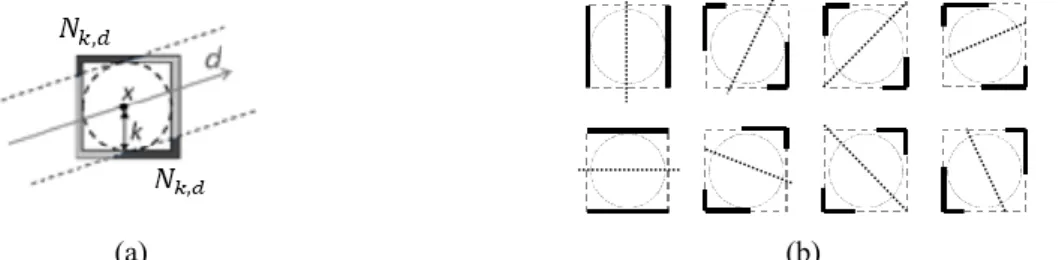
In the 2D case, a possible definition of 𝑁𝑘,𝑑(𝑥) is illustrated in Figure 8, where all the d directions considered
remain at the choice of the implementation.
(a) (b)
Fig. 8. Example of possible choices of the directional set 𝑁𝑘,𝑑: (a) for a given direction d (dark gray arrow); (b)
construction for 8 directions.
To illustrate this concept, Figure 9 shows the application of the principle of equation 11 to the segmentation of vessels in an eye fundus image. The value of k is chosen relative to the spatial resolution of the images in order to control the desired size of the selected structures.
(a) (b)
(c) (d)
Fig. 9. Example of segmentation of the vessels in an eye fundus image: (a) native image, (b) inverted grayscale image
(vessels in positive contrast), (c) segmented vessels by adaptive thresholding of the difference f - VLCFf, (d) superimposed segmentation.
2.2.2 Segmentation of 3D vascular structures
For vascular filtering in 3D space, we will choose the directional neighborhoods 𝑁𝑘,𝑑(𝑥) along planes oriented
orthogonal to different directions in space. In practice, we selected 9 spatial directions corresponding to the 18-connectivity (cf Figure 10).
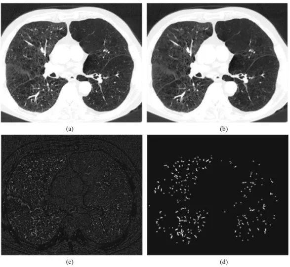
Figure 11 illustrates the result of 3D vascular filtering and the associated segmentation for filter size k = 3 on pulmonary CT data. The segmentation result in Figure 11d is obtained from the difference f - VLCFf (Figure
11c) by means of adaptive thresholding.
(a) (b)
Fig. 10. Illustration of the principle of 3D directional filtering; (a) asymmetrical orientations in 18-connectivity 𝐝𝐢∈ 𝐶18,
(b) example of orthogonal neighborhood 𝑁𝑘,𝑑(𝑥) for 𝒅 = 𝒅𝟒 in (a).
(a) (b)
(c) (d)
Fig. 11. Illustration of VLCFf (., k) on pulmonary 3D CT data at the level of an axial image (a), for k = 3: (b) filtered image, (c) difference, (d) segmented vascular structures (smaller than k in diameter).
The adaptive thresholding exploited, here called CHT (contrast hysteresis thresholding), adapts the principle of hysteresis thresholding, with an additional constraint that stops propagation of the segmentation if a local contrast condition is not respected.
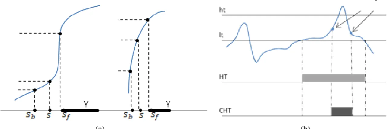
Considering an implementation of hysteresis thresholding in the form of an (iterative) binary reconstruction, let Y denotes the marking set selected by the high threshold ht (Y = {y ϵ supp (f) | (f (y) ≥ ht}), which will propagate within the set selected by the low threshold lt. If s denotes a point of the neighborhood of the segmented set Y at a given iteration, s will be added to the segmentation if the contrast with respect to its neighborhood V(s) in Y is smaller than the contrast computed with respect to the outer neighborhood, of lower value (Figure 12a) that is, if
𝑓(𝑠𝑓) − 𝑓(𝑠) ≤ 𝑓(𝑠) − 𝑓(𝑠𝑏) , (𝟏𝟐)
with 𝑠𝑓 ∈ 𝑌 ∩ V(s) and 𝑠𝑏 ∈ V(s) \𝑌 such as
𝑓(𝑠𝑏) < 𝑓(𝑠) . (𝟏𝟑)
This condition stops the propagation of the segmented set at the inflection points of the relief of f, even if the value of the low threshold is not reached, which better preserves the calibers of the vascular structures (Figure 12b).
(a) (b)
Fig. 12. Illustration of adaptive thresholding CHT. (a) left hand, configuration for which s is not added to Y and the
propagation stops; right hand, s will be added to Y and propagation will continue. (b) Comparison between hysteresis thresholding HT and contrast hysteresis thresholding CHT for two thresholds lt <ht.
2.2.3 Multi-scale approach for segmentation of 3D vascular structures
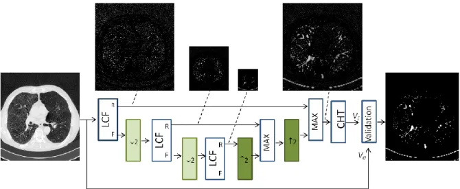
In order to remove / detect vascular structures of different sizes, the VLCF is applied in multi-resolution using 2 levels of decimation (Figure 13). Vascular structures are detected at each resolution level and combined together (MAX operator) before final adaptive thresholding by CHT and validation.
The detailed validation block (Figure 14b) is introduced to exploit the intrinsic contrast of the vascular structures with the objective of avoiding an overestimation of the calibers. It consists of applying the same type of CHT thresholding to the native data selected by the segmentation result obtained using multiresolution LCF filtering. The thresholds lt <ht are chosen according to the anatomical territory and the imaging modality considered and will be explained for each use case.
The final block of reconstruction by directional erosion guarantees the preservation of linear structures of a minimum length (minimum 2k, k being the size of VLCF filter) and the suppression of noise:
FD(𝑓)(𝑥) = 𝑅𝑓(𝑥, 𝑠𝑢𝑝𝑖{𝑓 ⊝ 𝐿𝒅𝑖}), 𝒅𝒊∈ C18 , (𝟏𝟒)
where 𝑅𝑓(. Y) denotes the reconstruction by dilation (here binary) of f with respect to the set Y V [20], ⊝ the
erosion and 𝐿𝒅𝑖 a line segment structuring element oriented in the direction 𝒅𝒊. In our case, 𝒅𝒊 denotes the set of
directions given by the 18-connectivity C18.
Fig 13. Multi-resolution VLCF filtering scheme applied to vascular detection. MAX denotes a re-composition block of the filtering results at different resolutions using the supremum operator, CHT a contrast thresholding by hysteresis and ↓ ↑ correspond to decimation and interpolation, respectively. The LCF and Validation blocks are detailed in Figure 14.
(a) LCF (b) « Validation » block
Fig. 14. Detail of the filter and post-processing blocks of the diagram of Figure 13. Filt. Dir denotes a directional filter block FD (eq.15) implementing reconstruction by directional erosion with a segment-type structuring element oriented in
several directions of space.
3. Results
We have applied the proposed approach to the detection of vascular structures in different clinical investigations using 3D imaging with and without contrast agent injection and quantified the results, namely for lung and liver. Note that the same segmentation scheme has been used in every case (Figure 13). The quantitative assessment was designed independently of the use case as follows: first a subset of 10 axial images evenly spaced in the 3D volume is selected. On each axial image, a ground truth was defined as a set of points falling in the vascular structures (true positives, VTP) and a set of points outside the vascular regions (true negatives, VTN) including various regions in the lung (liver) parenchyma (Figure 15).
The true positives TP detected by algorithms represent the number of VTP falling in the segmentation result. Similarly, the false positives FP detected by the algorithm represent the number of VTN falling in the
segmentation result. The false negatives (FN) are computed as the subtraction of the TP from the VTP, whereas the true negatives are given by TN = VTN - FP.
The reported quantitative scores were the sensitivity and the specificity: 𝑆𝐸𝑁𝑆 = [𝑇𝑃]
[𝑇𝑃] + [𝐹𝑁] ,
𝑆𝑃𝐸𝐶 = [𝑇𝑁]
[𝑇𝑁] + [𝐹𝑃] , (15)
(a) (b)
Fig. 15. Illustration of the quantitative assessment: (a) true positives VTP (green cross) and true negatives VTN (purple x);
(b) segmentation result (yellow) from which TP, FP, TN and FN are computed.
3.1 Intrapulmonary vascular tree segmentation
In the case of intrapulmonary vascular segmentation, the selection of parameters lt, ht in the flowchart Figure13 exploits the histogram of the intrapulmonary region (for which a mask is extracted cf. [24]) and corresponds to the range between the two modes of the histogram. Their values can be adapted according to the CT acquisition protocol used (here, lt = -900 HU, ht = -700 HU, Hounsfield Units). The quantitative evaluation was performed on the public database of the VESSEL12 challenge (20 patients) [23] by taking advantage of existing
annotations. Since the VESSEL12 submission website was closed at the time of this evaluation, we could not have a direct comparison with the results reported in [23] by using the same evaluation method. Nevertheless, we could compare with method B in [23] which belongs to our group. Upon request, we were provided with the ground truth annotations by the VESSEL12 organizers, including vessel and non-vessel (airway wall, mucus-filled bronchi, dense lesions, nodules) points. When re-evaluating method B on this database by considering the binary segmentation result (instead of probabilistic as used in [23]) we obtained different values for
sensitivity/specificity than in [23] (0.71/0.76 vs 0.68/0.99), probably due to the conversion from binary to probabilistic values for the segmentation, to which we do not have access. The sensitivity/specificity values of the proposed method obtained on the provided database (0.92/0.6) cannot thus be directly compared with the ones reported in [23]. Another aspect concerns the presence of 982 non-vessel (VTN) points in the annotation corresponding to lung nodules. Since the proposed approach does not include a post-processing step to remove such nodules, contrary to method B and other best-performing methods in [23], we decided to remove these VTN points from the ground truth and replace them with additional VTN points selected by a thoracic imaging expert from areas corresponding to lung fissures, ground glass, dense reticulations or dense lesions (when present), without duplicating existing annotations. For full transparency of evaluation, the sensitivity/specificity achieved by the proposed method versus method B on the provided VESSEL12 database while excluding nodule points was 0.92/0.73 vs 0.71/0.83.
Note that the non-inclusion of nodule regions in the ground truth does not bias the evaluation, for two reasons: first, we are able to detect juxtavascular nodules using the procedure developed in [25]; second, we consider preferable to preserve juxtavascular nodules in the segmentation, since otherwise we might remove other pertinent vascular deformations. For example, in the presence of pulmonary arterio-venous malformations, local vessel dilations similar with juxtavascular nodules occur and they have to be detected as part of vessels [25]. In conclusion, our evaluation database included VTP = 2249 vessel points (originally in the VESSEL12 database) and VTN = 6567 non-vessel points (non-vessel points in VESSEL12 database excluding lung nodules and including new annotations). On this database, the proposed method reached an average sensitivity/specificity of 0.92/0.83 compared with 0.71/0.86 obtained by method B in [23] (the same data preprocessing as in method B was applied, i.e. 3D Gaussian smoothing for acquisitions using high-frequency reconstruction kernels, namely case 01). Table 1 presents individual results per patient obtained by the proposed method. Two segmentation examples are shown in Figure 16.
Table 1. Evaluation result on lung dataset Patient 1 2 3 4 5 6 7 8 9 10 SENS 0.91 0.92 0.92 0.9 0.94 0.8 0.94 0.82 0.88 0.96 SPEC 0.71 0.89 0.7 0.86 0.9 0.93 0.85 0.85 0.83 0.87 Patient 11 12 13 14 15 16 17 18 19 20 SENS 0.97 0.9 0.96 0.9 0.98 0.97 0.78 0.98 1 0.95 SPEC 0.83 0.62 0.8 0.72 0.92 0.9 0.94 0.89 0.88 0.8
Fig. 16.Example of vascular detection in lung imaging at axial level and the associated 3D rendering for two patients.
The main advantage of the multiresolution VLCF method is that, besides preserving high accuracy in detecting small vessels, it is less sensitive with respect to noise and the presence of pathologies of positive-contrast appearance on the images (such as fibrosis and ground glass in the lung). This is particularly valuable for quantification and analysis of interstitial lung diseases which needs a clear distinction between normal vascular regions and pathological high opacities. Figure 17 shows an example of vascular segmentation in comparison with the previously developed approach [24] evaluated as method B in the VESSEL12 challenge [23].
3.2 Hepatic vascular tree segmentation
The same approach has been tested for vessel detection in hepatic imaging at various injection phases and for different noise/contrast rates in a 16 patients database. For this application, the parameters lt, ht in Figure 13 are similarly selected from the histogram of liver parenchyma; the liver mask is obtained with an independent method [26].
The ground truth for the quantitative evaluation includes an average of 158 VTP and 134 VTN for each liver acquisition, selected by a medical imaging expert. On this evaluation database, we obtained an average sensitivity/specificity of 0.88/0.94, cf Table 2. The qualitative analysis of the results reveals a good detection of vessels despite of the variable level of contrast (Figure 18).
(a) original axial CT (b) method B in [23] (c) proposed approach
Fig. 17. Segmentation illustration for a case of pulmonary fibrosis (top) and asthma (bottom) (a). Comparison between a competing approach [23] (b) and the one proposed (c), the latter showing less false positives in fibrosis areas (top) and
more true positives in blurred acquisitions (bottom).
Fig. 18. Example of vascular detection in liver imaging at axial level and associated 3D rendering (three patients). Only
Table2. Evaluation result on liver dataset Patient 1 2 3 4 5 6 7 8 SENS 1 1 0.81 0.91 0.88 0.9 0.7 0.9 SPEC 0.98 0.99 0.98 0.99 0.93 0.88 0.97 0.99 Patient 9 10 11 12 13 14 15 16 SENS 0.7 0.9 0.91 0.92 0.90 0.87 0.94 0.81 SPEC 0.92 0.81 0.93 0.89 0.95 0.96 0.88 0.87
1.1 Coronary arteries segmentation
A preliminary result for the segmentation of the coronary arteries (computed tomography CT acquisition with contrast injection, ECG synchronized) is shown in Figure 19. This was achieved after an interactive selection of the structures of interest, replacing the validation block in Figure 13. For this type of application, the post-processing (to be implemented in future work) will involve the segmentation of the peripheral regions of the heart for automatic coronary selection.
(a) (b)
Fig. 19. Preliminary result of the coronary arteries segmentation from a
clinical acquisition in coroscanner.
4. Discussion
The proposed method exploits prior knowledge about the vessel appearance on images, namely, curvilinear shape and positive contrast with respect to surrounding tissues. It relies on a local filtering step which consists of reconstructing the intensity value of a point based on existing connection paths with points of high intensity values in its neighborhood (defined at a given distance from the point, which corresponds to the filter size). In other words, the reconstructed point value results from the propagation of neighboring point values on high intensity paths when these exist. By considering the infimum reconstruction value of the point according to various spatial orientations of the neighborhood, points on curvilinear structures (vessels) will result with attenuated values (the maximum attenuation being achieved for an orthogonal neighborhood with respect to the vessel tangent). The vessel occurrence likelihood is given by the difference between the original and filtered images.
Such idea of computing structure “vesselness” by means of filtering is encountered in other approaches, the most famous being those exploiting Hessian-based curvature computation [14][27][28]. The proposed approach would however provide higher response at vessel bifurcations than Hessian-based filtering and still preserve low response in case of sheet-like or blob-like structures (smaller than the filter size) since for the latter ones a high-value connection path between the central point and the neighborhood will be preserved, no matter the spatial orientation of the neighborhood (note that for the 3D applications, the spatial neighborhood of a point is defined along a plane). Like other multi-scale approaches, the proposed approach applies the local filtering at different spatial resolutions (three levels of decimation in our case) in order to deal with different vessel calibers. Our method presents also some limitations. Because of the multi-scale approach, positive-contrast structures which are not vessels might be selected at a coarse scale, such as isolated nodules or dense opacities. Note however that most of them, if isolated from other vascular structures, can be easily removed by selecting only those presenting a minimal length on their skeleton (this post-processing was not applied in this paper, which could explain a lower specificity in the quantitative evaluation). Our approach cannot neither distinguish non-vessel structures if they have shape and contrast properties similar with non-vessels, which is the case, for example, for mucus-filled bronchi. To our knowledge, such limitation remains also valid for the other methods.
reconstruction-based filtering) involved at different scales. According to the algorithm implementation for the 2D grayscale reconstruction by dilation, its complexity varies from O(N x N) (sequential implementation) to
O(N log N) (for Union-Find implementation) [12], N denoting the number of points in the image. In our case, the reconstruction by dilation is performed on a 2D small filtering window (most generally being 7 x 7 pixels large) centered on each 3D image point and oriented in a given spatial direction, among 9 possible directions (Fig. 10). Since this local filtering is performed in parallel for the 9 directions, the complexity of the LCF filtering step (Fig. 13) is O(N x W2), where N is the number of the 3D image points (voxels) and W the number
of filtering window points. LCF being applied at three levels of decimation (at each decimation the image size being divided by 8) the downsampling path (Fig. 13) involves (N + N/8 + N/64) x W2 operations, which
corresponds to a complexity of O(N x W2).
The upsampling path of the Fig. 13 consists of interpolation and contrast hysteresis thresholding (CHT). Considering 8 neighbors for interpolation and 26 neighbors for CHT, the upsampling path involves 8 x (N/64 + N/8) + N/8 + N + 26 x N operations, i.e. a complexity of O(N). The final validation bloc involves 26 x N + N x sqrt(W) x 9 operations, that is a complexity of O(N x sqrt(W)).
Summing up, and denoting L = sqrt(W), the algorithm complexity for a 3D dataset containing N points (voxels) and a filtering window of L x L points, is O(N x L4). In practice, because of the small filter window size L,
complex image configurations (similar with the Peano curve) are unlikely to occur and even sequential
implementation of the grayscale reconstruction will have a smaller complexity (between O(W) and O(W log W)) which leads to a more likely global algorithm complexity of O(N x (L2 log L)). The algorithm average running
time for a dataset of VESSEL12 challenge is 20 minutes on a laptop PC equipped with Intel i7-8650U CPU E5-1607 @ 1.9 GHz.
5. Conclusion
In this paper we presented an original and generic vascular detection and segmentation framework based on multiresolution locally connected filtering. This approach, currently validated in two anatomical regions, has already been applied in the analysis of vascular remodeling in lung fibrosis [29] with promising results for biomarkers selection.
In conclusion, locally connected filters appear as an efficient alternative for automatic detection of vascular structures in various medical imaging modalities.
Acknowledgement
This work was funded by the French Grant PIA-CISN2 IMPACTumors.
The authors would like to thank the organizers of VESSEL12 challenge for providing the evaluation ground truth prior to its public release.
References
[1]Suri JS, Liu K, Reden L, Laxminarayan S. A review on MR vascular image processing algorithms: Acquisition and prefiltering: Part I. IEEE Transactions on Information Technology in Biomedicine 2002; 6(4):324–337.
[2] Suri JS, Liu K, Reden L, Laxminarayan S. A review on MR vascular image processing algorithms: Skeleton versus nonskeleton approaches: Part II. IEEE Transactions on Information Technology in Biomedicine 2002; 6(4):338–350.
[3] Kirbas and Quek. A review of vessel extraction techniques and algorithms. ACMComputing Surveys 2004; 36(2):81–121.
[4] Lesage D, Angelini ED, Bloch I, Funka-Lea G. A review of 3D vessel lumen segmentation techniques: Models, features and extraction schemes. Medical Image Analysis 2009; 13(6):819–845.
[5] Tankyevych O. Filtering of thin objects, applications to vascular image analysis [dissertation].University Paris-Est, France; 2010.
[6] Moccia S, De Momi E, El Hadji S, Mattos LS. Blood vessel segmentation algorithms - Review of methods, datasets and evaluation metrics. Computer Methods and Programs in Biomedicine 2018; 158: 71-91.
[7] Zucker S. Region growing: Childhood and adolescence. Computer Graphics and Image Processing 1976; 5(3):382–399.
[8] Tyrrell JA, di Tomaso E, Fuja D, Tong R, Kozak K, Jain RK, et al. Robust 3-D modeling of vasculature imagery using superellipsoids. IEEE Transactions on Medical Imaging 2007; 26(2):223–237.
[9] Lorigo LM, Faugeras OD, Grimson WE, Keriven R, Kikinis R, Nabavi A et al. Curves: Curve evolution for vessel segmentation. Medical Image Analysis 2001; 5(3):195–206.
[10] Olabarriaga S.D., Breeuwer M., Niessen W.J. Minimum cost path algorithm for coronary artery central axis tracking in CT images.In: Ellis R.E., Peters T.M, editors. Medical Image Computing and Computer-Assisted Intervention - MICCAI 2003. MICCAI 2003. Lecture Notes in Computer Science. Springer, Berlin, Heidelberg; 2003. 2879:687–694.
[11] Manniesing R, Viergever M, Niessen, W.J. Vessel axis tracking using toplogy constrained surface evolution. IEEE Transactions on Medical Imaging. 2007;26(3):309–316.
[12] Najman and Talbot. Mathematical Morphology: From theory to applications. 1st ed. J.Wiley & Sons, editor. 2010
[13] Wong WC, Chung AC. Probabilistic vessel axis tracing and its application to vessel segmentation with stream surfaces and minimum cost paths. Medical Image Analysis 2007; 11(6):567–587.
[14]Frangi A, Niessen W, Vincken K, Viergever M. Multiscale vessel enhancement filtering.In: Wells W.M., Colchester A., Delp S., editors. Medical Image Computing and Computer-Assisted Intervention — MICCAI 1998. MICCAI 1998. Lecture Notes in Computer Science, vol 1496. Springer, Berlin, Heidelberg;
1998.1946:130–137.
[15] Zheng Y, Loziczonek M, Georgescu B, Zhou K, Vega-Higuera F; Comaniciu D. Machine learning based vesselness measurement for coronary artery segmentation in cardiac CT volumes. In: Dawant B, Haynor D, editors. Image Processing. Proceedings of SPIE 7962, Medical Imaging 2011; 2011. 7962:79 621K–1. [16] Oliveira DA, Feitosa RQ, Correia MM. Segmentation of liver, its vessels and lesions from CT images for surgical planning. Biomed Eng Online 10,30.2011
[17] Zhang J, Tang Z., Gui W, Liu J. Retinal vessel image segmentation based on correlational open active contours model. 2015 Chinese Automation Congress (CAC)2015; 993-998.
[18] Orkisz M, Hoyos M, Romanello V, Romanello C, Prieto J., Revol-Muller,C. Segmentation of the pulmonary vascular trees in 3D CT images using variational region-growing. IRBM 2014; 35:11-19.
[19] Tian Y, Chen Q, Wang W, Peng Y, Wang Q, Duan Fuqing et al. A Vessel Active Contour Model for Vascular Segmentation. BioMed research international. 2014.
[20] Vincent L.Morphological grayscale reconstruction in image analysis: applications and efficient algorithms.IEEE Trans. on Image Processing 1993; 2: 176-201.
[21] Smistad E, Elster Anne, Lindseth Frank. Smistad, Erik & Elster, Anne & Lindseth, Frank. GPU accelerated segmentation and centerline extraction of tubular structures from medical images. International journal of computer assisted radiology and surgery. 2013
[22] Lassen B, van Rikxoort EM, Schmidt M, Kerkstra S, van Ginneken B, Kuhnigk JM. Automatic
Segmentation of the Pulmonary Lobes From Chest CT Scans Based on Fissures, Vessels, and Bronchi. IEEE Transactions on Medical Imaging. 2013; 32(2):210-222.
[23] Rudyanto RD, Kerkstra S, van Rikxoort EM, Fetita C, Brillet PY, Lefevre Cnet al. Comparing algorithms for automated vessel segmentation in computed tomography scans of the lung: The VESSEL12 study. Medical Image Analysis. 2014;18:1217-32.
[24] Fetita C, Brillet P-Y, Preteux F. Morpho-geometrical approach for 3D segmentation of pulmonary vascular tree in multi-slice CT. SPIE Medical Imaging 2009: Image Processing. 2009.72594F.
[25] Fetita C, Fortemps de Loneux T, Kouvahe A, El Hajjam M, Automatic detection and quantification of pulmonary arterio-venous malformations in hereditary hemorrhagic telangiectasia, SPIE Medical Imaging 2017: Computer-Aided Diagnosis, Feb 2017, pp.1013419-1 - 1013419-9.
[26] Fetita C, Lucidarme O, Preteux F, Grenier P. CT hepatic venography: 3D vascular segmentation for preoperative evaluation. Proceedings 8th International Conference on MICCAI'05. 2005; 2: 830-837.
[27] Sato, Y., Nakajima, S., Shigara, N., Atsumi, H., Koller, T., Gerig, G., Kikinis, R. Three-dimensional multi-scale line filter for segmentation and visualization of curvilinear structures in medical images. Medical Image Analysis 2 1998; 143-168.
[28] Krissian, K., Malandain, G., Ayache, N., Vaillant, R., Trousset, Y. Model based detection of tubular structures in 3D images. Computer Vision and Image Understanding 80 2000; 130-171.
[29] Kim Y-W, Tarando S, Brillet P-Y, Fetita C. Image biomarkers for quantitative analysis of idiopathic interstitial pneumonia.SPIE Medical Imaging 19: Computer-Aided Diagnosis, Feb 2019. 2019; 10950-44.