HAL Id: hal-01587438
https://hal.archives-ouvertes.fr/hal-01587438
Submitted on 20 Apr 2018
HAL is a multi-disciplinary open access
archive for the deposit and dissemination of
sci-entific research documents, whether they are
pub-lished or not. The documents may come from
teaching and research institutions in France or
abroad, or from public or private research centers.
L’archive ouverte pluridisciplinaire HAL, est
destinée au dépôt et à la diffusion de documents
scientifiques de niveau recherche, publiés ou non,
émanant des établissements d’enseignement et de
recherche français ou étrangers, des laboratoires
publics ou privés.
totalcolumn CH4 and CO2 for 2009 and 2010
Sudhanshu Pandey, Sander Houweling, Maarten Krol, Ilse Aben, Frédéric
Chevallier, Edward J. Dlugokencky, Luciana V. Gatti, Emanuel Gloor, John
B. Miller, Rob Detmers, et al.
To cite this version:
Sudhanshu Pandey, Sander Houweling, Maarten Krol, Ilse Aben, Frédéric Chevallier, et al.. Inverse
modeling of GOSAT-retrieved ratios of totalcolumn CH4 and CO2 for 2009 and 2010. Atmospheric
Chemistry and Physics, European Geosciences Union, 2016, 16 (8), pp.5043 - 5062.
�10.5194/acp-16-5043-2016�. �hal-01587438�
www.atmos-chem-phys.net/16/5043/2016/ doi:10.5194/acp-16-5043-2016
© Author(s) 2016. CC Attribution 3.0 License.
Inverse modeling of GOSAT-retrieved ratios of total column CH
4
and CO
2
for 2009 and 2010
Sudhanshu Pandey1,2, Sander Houweling1,2, Maarten Krol1,2,3, Ilse Aben2, Frédéric Chevallier4,
Edward J. Dlugokencky5, Luciana V. Gatti6, Emanuel Gloor7, John B. Miller5,8, Rob Detmers2, Toshinobu Machida9, and Thomas Röckmann1
1Institute for Marine and Atmospheric Research Utrecht, Utrecht University, Utrecht, the Netherlands 2SRON Netherlands Institute for Space Research, Utrecht, the Netherlands
3Department of Meteorology and Air Quality (MAQ), Wageningen University and Research Centre,
Wageningen, the Netherlands
4Laboratoire des Sciences du Climat et de l’Environnement (LSCE), CEA CNRS UVSQ, IPSL, Gif-sur-Yvette, France 5NOAA Earth System Research Laboratory, Boulder, Colorado, USA
6Instituto de Pesquisas Energéticas e Nucleares (IPEN), Centro de Química Ambiental, São Paulo, Brazil 7School of Geography, University of Leeds, Leeds, UK
8Cooperative Institute for Research in Environmental Sciences (CIRES), University of Colorado, Boulder, Colorado, USA 9National Institute for Environmental Studies, Tsukuba, Japan
Correspondence to: Sudhanshu Pandey (s.pandey@uu.nl)
Received: 25 January 2016 – Published in Atmos. Chem. Phys. Discuss.: 3 February 2016 Revised: 4 April 2016 – Accepted: 6 April 2016 – Published: 22 April 2016
Abstract. This study investigates the constraint provided by
greenhouse gas measurements from space on surface fluxes. Imperfect knowledge of the light path through the atmo-sphere, arising from scattering by clouds and aerosols, can create biases in column measurements retrieved from space. To minimize the impact of such biases, ratios of total column retrieved CH4 and CO2 (Xratio) have been used. We apply
the ratio inversion method described in Pandey et al. (2015) to retrievals from the Greenhouse Gases Observing SATel-lite (GOSAT). The ratio inversion method uses the measured Xratio as a weak constraint on CO2 fluxes. In contrast, the
more common approach of inverting proxy CH4 retrievals
(Frankenberg et al., 2005) prescribes atmospheric CO2fields
and optimizes only CH4fluxes.
The TM5–4DVAR (Tracer Transport Model version 5– variational data assimilation system) inverse modeling sys-tem is used to simultaneously optimize the fluxes of CH4
and CO2 for 2009 and 2010. The results are compared to
proxy inversions using model-derived CO2 mixing ratios
(XCOmodel2 ) from CarbonTracker and the Monitoring Atmo-spheric Composition and Climate (MACC) Reanalysis CO2
product. The performance of the inverse models is
evalu-ated using measurements from three aircraft measurement projects.
Xratioand XCOmodel2 are compared with TCCON retrievals
to quantify the relative importance of errors in these com-ponents of the proxy XCH4 retrieval (XCHproxy4 ). We find
that the retrieval errors in Xratio (mean = 0.61 %) are
gen-erally larger than the errors in XCOmodel2 (mean = 0.24 and 0.01 % for CarbonTracker and MACC, respectively). On the annual timescale, the CH4fluxes from the different satellite
inversions are generally in agreement with each other, sug-gesting that errors in XCOmodel2 do not limit the overall ac-curacy of the CH4flux estimates. On the seasonal timescale,
however, larger differences are found due to uncertainties in XCOmodel2 , particularly over Australia and in the tropics. The ratio method stays closer to the a priori CH4flux in these
re-gions, because it is capable of simultaneously adjusting the CO2fluxes. Over tropical South America, comparison to
in-dependent measurements shows that CO2fields derived from
the ratio method are less realistic than those used in the proxy method. However, the CH4fluxes are more realistic, because
the impact of unaccounted systematic uncertainties is more evenly distributed between CO2and CH4. The ratio
inver-sion estimates an enhanced CO2release from tropical South
America during the dry season of 2010, which is in accor-dance with the findings of Gatti et al. (2014) and Van der Laan et al. (2015).
The performance of the ratio method is encouraging, be-cause despite the added nonlinearity due to the assimilation of Xratioand the significant increase in the degree of freedom
by optimizing CO2fluxes, still consistent results are obtained
with respect to other CH4inversions.
1 Introduction
Detailed knowledge of the global distribution of surface fluxes of potent greenhouse gases (GHGs) such as CH4
and CO2 is needed to investigate the uncertain feedback
of the global carbon cycle to human disturbances. Atmo-spheric measurements of these GHGs can provide informa-tion about the atmospheric budget. Inverse modeling meth-ods, also known as top-down approaches, have been devel-oped to make use of that information to obtain improved es-timates of surface fluxes. Bottom-up eses-timates of those fluxes are used as prior values in the top-down method, and are fur-ther improved using atmospheric measurements. Inversions assimilating flask and/or in situ measurements from surface networks have significantly improved our knowledge of the sources and sinks of GHGs (Bousquet et al., 2006; Bergam-aschi et al., 2010; Hein et al., 1997; Houweling et al., 1999; Peters et al., 2007; Chevallier et al., 2010; Gurney et al., 2008). However, many regions with a key role in the global annual budgets of CO2and CH4are not adequately covered
by the surface measurement network. This is especially true for tropical regions and the Southern Hemisphere.
The Greenhouse Gases Observing SATellite (GOSAT) is the first satellite dedicated to monitoring GHGs from space (Kuze et al., 2009; Yokota et al., 2009; Yoshida et al., 2011). Onboard are the Thermal And Near infrared Sen-sor for carbon Observation-Fourier Transform Spectrome-ter (TANSO-FTS) and a dedicated Cloud and Aerosol Im-ager (TANSO-CAI). TANSO-FTS measures the absorption spectra of Earth-reflected sunlight in the shortwave infrared (SWIR) spectral range, from which XCO2and XCH4are
re-trieved with global coverage. Several inverse modeling stud-ies have applied these measurements to derive constraints on the surface fluxes of CH4and CO2(Alexe et al., 2015; Basu
et al., 2013; Deng et al., 2014; Maksyutov et al., 2012; Berga-maschi et al., 2013; Fraser et al., 2013; Houweling et al., 2015; Monteil et al., 2013; Turner et al., 2015).
Systematic errors in satellite retrievals are an important factor limiting the scientific interpretation of the data, and various methods have been proposed to mitigate their im-pact on the inferred surface fluxes (Bergamaschi et al., 2007; Frankenberg et al., 2005; Butz et al., 2010; Parker et al., 2015). An important source of systematic error is the
scat-tering of light by aerosols and thin cirrus clouds along the measured light path. Two types of retrieval methods have been developed in the past to account for atmospheric scat-tering, referred to as the full-physics and proxy approach. The full-physics approach tries to account for scattering-induced errors by explicitly modeling the scattering pro-cess, and retrieving scattering properties from the data (Butz et al., 2010). The proxy method, first introduced by Franken-berg et al. (2005), takes the ratio of XCH4 and XCO2
re-trieved at nearby wavelengths (1562 to 1585 nm for XCO2
and 1630 to 1670 nm for XCH4) so that path length
pertur-bations due to atmospheric scattering largely cancel out in the ratio (see Eq. 1). Xratiois multiplied with model-derived
XCO2(XCOmodel2 ) to derive XCH4(XCHproxy4 ) (see Eq. 2).
Xratio=
XCH4ns
XCO2ns
(1)
XCH4proxy=Xratio×XCO2model (2)
Here, XCHns4 and XCOns2 are retrieved assuming a non-scattering atmosphere. XCOmodel2 is calculated using a trans-port model, normally employing CO2 surface fluxes that
have been optimized using surface measurements. The at-mospheric CO2 fields are sampled at the coordinates of
the satellite measurements and converted to corresponding total columns using the retrieval-derived averaging kernels (Schepers et al., 2012).
Proxy XCH4 retrievals from GOSAT have been used in
many inverse modeling studies to investigate the global sur-face fluxes of CH4(Alexe et al., 2015; Monteil et al., 2013;
Fraser et al., 2013; Bergamaschi et al., 2013). These stud-ies rely on the assumption that the uncertaintstud-ies and biases in XCOmodel2 are relatively unimportant. Some recent studies have investigated this assumption in further detail. Schepers et al. (2012) suggested that the errors in XCHproxy4 are mostly dominated by the errors in XCOmodel2 . Pandey et al. (2015) did a series of Observing System Simulation Experiments to quantify the impact of errors in XCOmodel2 on inversion-derived CH4fluxes. It was concluded that the error becomes
significant when CO2 fluxes are poorly constrained by the
surface measurements. Parker et al. (2015) have estimated the uncertainty in XCOmodel2 by comparing values from dif-ferent models. They found that the uncertainty in XCOmodel2 becomes the most important term in the error budget of XCHproxy4 retrieval during summer months, when the satellite instrument operates under favorable illumination conditions, allowing accurate determination of Xratio.
In an attempt to avoid the biases introduced by errors in XCOmodel2 , Fraser et al. (2014) developed the ratio method, which simultaneously constrains CO2and CH4fluxes by
as-similating Xratio on the subcontinental scale using the
en-semble Kalman filter. Pandey et al. (2015) also developed a similar ratio inversion method for jointly optimizing the
surface fluxes of CH4and CO2 on the model grid scale
us-ing a variational optimization method. Fraser et al. (2014) compared posterior CH4and CO2flux uncertainties derived
from a ratio inversion with traditional CH4proxy and CO2
full-physics inversions and reported a larger reduction in un-certainty than the two in the tropics for the fluxes of both tracers.
This study extends the work of Pandey et al. (2015), by separately inverting real GOSAT measurements of Xratio
and XCHproxy4 in a consistent and comparable framework to investigate the following questions. (1) How do errors in XCOmodel2 influence the results of a XCHproxy4 inver-sion? (2) How does the Xratio inversion system developed
by Pandey et al. (2015) perform using real data? The perfor-mance of the inversions is evaluated using independent air-craft measurements. We provide an estimate of the posterior uncertainties of the Xratio-inverted fluxes using the Monte
Carlo method described by Chevallier et al. (2007).
This paper is organized as follows. The following section explains the methods used in this study. Section 2.1 describes the inverse model and the a priori flux assumptions. Sec-tion 2.2 lists the measurements that are assimilated in the inversions and used for validation. Section 2.3 provides an overview of the inversions performed in the study. Section 3 presents the inversion results and Sect. 4 discusses their im-plications for the use of satellite retrievals in inversion stud-ies. Finally, we give the overall conclusions of this work.
2 Method
We invert GOSAT retrievals of Xratio and XCHproxy4 , each
together with flask-air CH4 and CO2 measurements from
the NOAA Global Greenhouse Gas Reference Network (GGGRN) to provide monthly surface fluxes of CO2 and
CH4 using the TM5–4DVAR inversion system (Meirink
et al., 2008). This is done as follows.
1. GOSAT-retrieved total column measurements of Xratio
are compared to measured ratios of XCH4: XCO2from
the Total Carbon Column Observing Network (TC-CON) of ground-based sun-tracking Fourier transform spectrometers (FTSs) (Wunch et al., 2011).
2. GOSAT Xratio measurements are bias corrected by
fit-ting a linear function of surface albedo to the residual differences between GOSAT and TCCON. This is done in Xratiospace.
3. GOSAT Xratio measurements are multiplied by
XCOmodel2 to generate XCHproxy4 measurements. Two different versions of XCOmodel2 are used (see Sect. 2.2) to investigate the sensitivity to model errors.
4. The XCHproxy4 and Xratio measurements are inverted
along with surface observations and the resulting
pos-terior surface fluxes are integrated over the TransCom regions (see Fig. S4 in the Supplement).
5. The posterior flux uncertainty for all inversions is quan-tified using a Monte Carlo approach (see Appendix B) for consistent comparison.
6. The performance of the inversions is evaluated and compared using independent aircraft measurements. The remainder of this section explains these steps in fur-ther detail.
2.1 Inversion setup
We use the TM5–4DVAR inversion modeling system. It is comprised of the Tracer Transport Model version 5 (TM5; Krol et al., 2005) coupled to a variational data assimilation system (4DVAR; Meirink et al., 2008). TM5 simulates the spatiotemporal distribution of a tracer in the atmosphere for a given set of fluxes. In this study, TM5 is run at a 6◦×4◦ horizontal resolution and 25 vertical hybrid sigma pressure levels from the surface to the top of the atmosphere. The meteorological fields for this offline model are taken from the European Centre for Medium-Range Weather Forecasts (ECMWF) ERA-Interim reanalysis (Dee et al., 2011).
CH4fluxes are optimized as a single flux category,
repre-senting the sum of all processes. For CO2, biospheric and
oceanic fluxes are optimized separately. The a priori CH4
fluxes used in the study are the same as used in Houwel-ing et al. (2014), except for the anthropogenic fluxes. We use the v.4.2FT2010 version of EDGAR (European Commission, Joint Research Centre (JRC)/Netherlands Environmental As-sessment Agency), whereas Houweling et al. (2014) use ver-sion 4.1. The a priori CO2fluxes come from CarbonTracker,
CT2013B (Peters et al., 2007), in which biosphere fluxes are based on the Carnegie-Ames-Stanford Approach (CASA) biogeochemical model, fire fluxes are based on the Global Fire Emissions Database v3.1 (GFED), and ocean fluxes are based on Jacobson et al. (2007). Fossil fuel fluxes in Carbon-Tracker are based on the Miller module (Tans et al., 2014). The a priori flux covariance matrix is constructed assuming relative flux uncertainties of 50, 84, and 60 % per grid box and month for the total CH4, biospheric CO2, and oceanic
CO2 categories, respectively. The fluxes are assumed to be
correlated temporally using an exponential correlation func-tion with temporal scales of 3, 3, and 6 months, respectively, and spatially with Gaussian functions using corresponding length scales of 500, 500, and 3000 km for total CH4,
bio-spheric CO2, and oceanic CO2, respectively.
2.2 Measurements
Here we give a brief account of the measurements that were assimilated (GOSAT and NOAA) or used for validation (TC-CON and aircraft measurements).
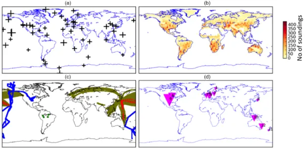
Figure 1. Measurements used in this study. (a) The crosses indicate the locations of NOAA surface sampling sites. The lengths of the vertical and horizontal bars are proportional to the number of CO2and CH4measurements, respectively. (b) The number of GOSAT soundings binned
at 1◦×1◦for the time period of June 2009 to December 2010; (c) flight tracks of the aircraft campaigns HIPPO 2 and 3 (blue), CONTRAIL CO2(olive), CONTRAIL CH4(red), and AMAZONICA (green); (d) the locations of the TCCON measurement sites. The numbers (1–12)
refer to corresponding entries in Table 1. The size of the purple rectangles is proportional to the number of collocated high-gain GOSAT soundings.
2.2.1 GOSAT
The XCHns4 and XCOns2 terms in Eq. (1) were taken from the RemoTeC XCH4 Proxy retrieval v2.3.5 (Butz et al.,
2011). More information about the data set can be found in the Product User Guide on the ESA GHG CCI web-site (Detmers and Hasekamp, 2014). The RemoTeC al-gorithm uses GOSAT TANSO-FTS NIR and SWIR spec-tra to retrieve XCHns4 and XCOns2 simultaneously, assum-ing a non-scatterassum-ing atmosphere (Schepers et al., 2012). Xratiovalues were translated into XCHproxy4 using XCOmodel2
derived from the following: (1) Monitoring Atmospheric Composition and Climate (MACC) reanalysis CO2
prod-uct (www.copernicus-atmosphere.eu). It uses Laboratoire de Météorologie Dynamique transport model (LMDZ) (Cheval-lier, 2013). The corresponding XCHproxy4 product will be referred to as XCHma4 . (2) XCOmodel2 is derived from CarbonTracker-2013B (http://www.esrl.noaa.gov/gmd/ccgg/ carbontracker/). These CO2 fields are calculated using the
TM5 model as used in this study. The corresponding XCHproxy4 product will be referred to as XCHct4.
Both data assimilation systems optimized the CO2fluxes
using surface measurements of CO2. For GOSAT
measure-ments, we only used the high-gain soundings from GOSAT under cloud-free conditions from nadir mode. This was done to avoid any systematic inconsistency among the operation modes of TANSO. Figure 1 shows the spatial coverage of the GOSAT data set used in our inversions.
Systematic mismatches between NOAA-optimized and GOSAT-optimized TM5 CH4fields were observed by
Mon-teil et al. (2013). We apply another bias correction (in ad-dition to TCCON-based bias correction applied to Xratio) to
Xratioand XCHproxy4 by comparing them to total column CH4
and CO2optimized via an inversion using TM5–4DVAR and
NOAA flask-air data (see Appendix A).
2.2.2 TCCON
TCCON is a global network of ground-based FTS instru-ments for measuring the total column abundance of several gases, including XCO2 and XCH4, in the near infrared
re-gion of the electromagnetic spectrum (Wunch et al., 2011). These measurements are the standard for validating total column retrievals from greenhouse-gas-observing satellites such as GOSAT. We validate XCHns4, XCOns2, Xratio, XCOma2 ,
and XCOct2 with corresponding values of XCH4, XCO2, and
XCH4: XCO2 measured by TCCON at 12 sites using the
GGG2014 release of the TCCON data set (see Fig. 1 and Sect. 3.1). An albedo-based bias correction was applied to GOSAT-retrieved Xratio to account for the mismatch with
TCCON Xratio(see Appendix A).
2.2.3 NOAA
High-accuracy surface measurements of CH4and CO2were
used from NOAA’s GGGRN (Dlugokencky et al., 2015). The standard scale used for CO2is the WMO X2007 scale and for
CH4is the WMO X2004 scale. Only the sites with
continu-ous data coverage (on a roughly weekly basis) without gaps in the time period of 1 June 2009 to 31 December 2010 were included. A total of 8552 CH4observations and 7843 CO2
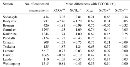
Table 1. TCCON validation of the components of XCHproxy4 (see Eq. 2). The numbers represent mean percentage differences with TCCON (weighted with TCCON + GOSAT error). A negative number means that the satellite retrieval is lower than TCCON. Data from these stations were used: Sodankylä (Kivi et al., 2014), Białystok (Deutscher et al., 2014a), Bremen (Deutscher et al., 2014b), Garmisch (Sussmann and Rettinger, 2014), Karlsruhe (Hase et al., 2014), Parkfalls (Wennberg et al., 2014a), Orleans (Warneke et al., 2014), Tsukuba (Morino et al., 2014), Lamont (Wennberg et al., 2014b), Darwin (Griffith et al., 2014a), Lauder (Sherlock et al., 2014), and Wollongong (Griffith et al., 2014b), and are arranged from north to south (for TCCON site locations, see Fig. 1).
Station No. of collocated Mean differences with TCCON (%) measurements XCO2ns XCH4ns Xratio XCO2ct XCO2ma
Sodankylä 434 −3.03 −2.81 0.21 0.68 0.34 Białystok 731 −2.46 −1.79 0.62 0.31 0.05 Bremen 426 −1.81 −0.99 0.76 −0.05 −0.32 Garmisch 1295 −1.93 −1.09 0.76 0.40 0.05 Karlsruhe 1244 −1.74 −1.00 0.69 0.15 −0.25 Parkfalls 2174 −1.23 −0.43 0.75 0.22 0.11 Orleans 808 −1.53 −0.75 0.75 0.21 −0.09 Tsukuba 135 −1.87 −1.24 0.63 0.57 −0.03 Lamont 5617 −0.73 −0.03 0.68 0.07 −0.00 Darwin 1065 −0.67 −0.19 0.47 0.02 0.14 Lauder 110 −1.05 −0.57 0.46 0.14 0.03 Wollongong 1515 −0.81 −0.45 0.35 0.10 0.00
observations were used from the same 51 sites. Figure 1 shows the location of the observation sites. 1σ uncertainties of 0.25 ppm and 1.4 ppb were assigned to CO2and CH4
mea-surements, respectively (Basu et al., 2013; Houweling et al., 2014). Note that our system also assigns a modeling error to each observation depending on simulated local gradients in mixing ratio (Basu et al., 2013). Modeling error values have a mean of 27.5 ppb, 2.72 ppm (and 1σ of 25.5 ppb, 4 ppm) for CH4and CO2, respectively.
2.2.4 Aircraft measurements
Airborne measurements from various aircraft measurement projects were used to test the inversion optimized model (see Sect. 3.2.5). The following projects have been used:
1. HIAPER Pole-to-Pole Observations (HIPPO) from Wofsy et al. (2012a);
2. Comprehensive Observation Network for TRace gases by AIrLiner (CONTRAIL) from Machida et al. (2008); 3. IPEN aircraft measurements over Brazil (referred as
AMAZONICA) from Gatti et al. (2014).
HIPPO provides in situ measurements covering the verti-cal profiles of CO2and CH4over the Pacific, spanning a wide
range in latitude (approximately pole-to-pole), from the sur-face up to the tropopause. We used data from the HIPPO 2 (26 October to 19 December 2009) and HIPPO 3 (20 March to 20 April 2010) campaigns. The continuous in situ mea-surements of CH4 and CO2 that were used have been bias
corrected with flask-air samples that were collected during each flight and analyzed at NOAA (Wofsy et al., 2012b).This
allows us to make consistent comparison with our inver-sions models, as all of them assimilate NOAA flask mea-surements. CONTRAIL makes use of commercial airlines to measure in situ CO2by continuous measurement
equip-ment. For some of the CONTRAIL flights CH4
measure-ments are also available from flask-air samples. We use data from a lower-troposphere greenhouse-gas sampling program as part of the AMAZONICA project, over the Amazon Basin in 2010, measuring biweekly vertical profiles of CO2 and
CH4from above the forest canopy to 4.4 km above sea level
at four locations: Tabatinga (TAB), RioBranco (RBA), Alta Floresta (ALF), and Santarem (SAN) (Gatti et al., 2014). The coverage of all aircraft measurements that were used in this study is shown in Fig. 1.
2.3 Inversion experiments
The following inversions have been performed:
1. SURF: inversions assimilating flask-air measurements of CH4 or CO2 to constrain surface fluxes of CH4 or
CO2, respectively;
2. RATIO: inversion assimilating Xratioand flask-air
mea-surements of CH4and CO2to constrain surface fluxes
of CH4and CO2;
3. PR-MA: inversion assimilating proxy XCHma4 and flask-air measurements of CH4to constrain surface fluxes of
CH4;
4. PR-CT: inversion assimilating proxy XCHct4 and flask-air measurements of CH4to constrain surface fluxes of
To assess the relative performance of each inversion, we validate atmospheric concentrations as simulated using the optimized fluxes from the different inversions with aircraft measurements. We define a normalized chi-square statistic to quantify the agreement between the optimized model and aircraft measurements.
κ =1
n(y − Hx)
TR−1(y − Hx), (3)
where y is a vector of the aircraft measurements, n is the length of y. Hx is the TM5 simulation sampled at the mea-surement coordinates. The covariance matrix R represents the expected uncertainty in the model–data mismatch. Its di-agonal elements are calculated as the sum of the model rep-resentation error of TM5 and the measurement uncertainty; all non-diagonal elements are set to 0.
3 Results
3.1 GOSAT–TCCON comparison
TCCON measurements are used to investigate the errors in GOSAT-retrieved XCH4. Each term on the right-hand
side of Eq. (2) contributes to the uncertainty in XCHproxy4 . To quantify these error contributions, we compare TCCON measurements of Xratio, XCH4, and XCO2 to
correspond-ing co-located GOSAT-retrievals. The validation is carried out for the time period of 1 June 2009 to 31 December 2013, for which both proxy data sets (XCHma4 and XCHct4) are available. Table 1 shows mean differences per TC-CON station, expressed as fractional differences to facili-tate the comparison of quantities with different units. As expected, the largest differences between GOSAT and TC-CON are found for XCOns2 and XCHns4. In general, XCOns2 (mean = −1.57 %) shows larger relative differences than XCHns4 (mean = −0.95 %). A latitudinal dependence can be observed, with increasing biases towards stations at higher latitudes. This can be explained by increased aerosol sctering at larger sun angles, as the light path through the at-mosphere is longer. For all the stations, the mean differ-ence is negative which is expected for aerosol scattering-induced errors at the low surface albedos of the TCCON sites (Houweling et al., 2004). The smaller bias values for Xratio
than XCOns2 and XCHns4 confirm that scattering-induced er-rors cancel out in their ratio, which motivated the proxy ap-proach (Frankenberg et al., 2005). Overall, we observe that Xratio(mean bias = 0.59 %) is the larger contributor to the
er-ror in XCHproxy4 than MACC (XCOma2 , mean bias = 0.01 %) and CarbonTracker (XCOct2, mean bias = 0.24 %).
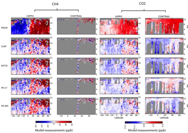
Figure 2. Fit residuals, comparing the performance of different in-versions. The top three rows show the difference between TM5– 4DVAR and GOSAT measurements (Xratiofor RATIO, XCHproxy4
for PR-CT and PR-MA), using a priori (left) and a posteriori (right) fluxes. The bottom row shows histograms of measurement–model mismatches between TM5–4DVAR and NOAA surface measure-ments in 400 bins between ±10σ range of the a priori mismatch.
3.2 Inversion results 3.2.1 Assimilation statistics
Figure 2 summarizes the statistics of the model– measurement comparison. The prior Xratio mismatches
typically fall in the range ±1 % (with mean = 0.007 ppb/ppm and 1σ = 0.043 ppb/ppm). The inversions reduce the average mismatch by about a factor of 10, and the variation of single column mismatches by about a factor of 2. The XCHproxy4 of PR-CT and PR-MA have bimodal prior mismatches, because the a priori model overestimates the north–south gradient of CH4. The bottom panels of Fig. 2 show mismatches
between TM5 and surface flask measurements of CH4 and
CO2. The CH4 a priori measurement mismatch has a mean
of −18.30 ppb and a 1σ of 42.30 ppb. The RATIO, SURF, PR-CT, and PR-MA inversions are all able to fit the NOAA data to a similar extent, reducing the a priori differences by more than a factor of 20. CO2 flask measurements are
assimilated in SURF and RATIO. Both inversions reduce the a priori mismatch (mean = −2.12 ppm, 1σ = 3.88 ppm), with RATIO (mean = −0.04 ppm, 1σ = 3.69 ppm) fitting
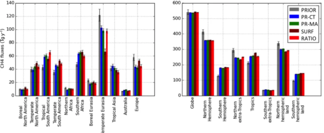
Figure 3. Annual fluxes of CH4integrated over different regions. The black line on each bar represents the ±1σ uncertainty.
the CO2 flask data as well as SURF (mean = −0.06 ppm,
1σ = 3.72 ppm).
3.2.2 CH4fluxes
Optimized annual CH4fluxes, integrated over the TransCom
regions are shown in the left panel of Fig. 3. The fluxes ob-tained with the RATIO inversion are on average more similar to fluxes from other GOSAT inversions than to the surface inversion, with a few exceptions. Differences between satel-lite and surface inversion are most prominent over tropical South America, where the latter is closer to the prior, which can likely be explained by the lack of surface measurement coverage. We will return to the inversion results for tropi-cal South America in Sect. 3.2.6, where validation results are shown using aircraft data.
The most significant difference between the satellite inver-sion and SURF is found for temperate Eurasia, where SURF reduces the CH4 fluxes from 121 Tg y−1 in the prior
esti-mate to 66 Tg y−1. When satellite data are added, the fluxes increase again to 100 Tg y−1. The large flux correction in the SURF inversion is compensated by increases in other TransCom regions of 5–10 Tg y−1(see for example temper-ate North and South America). In those regions stemper-atellite in-versions remain closer to the prior than the SURF inver-sion, which may well be driven by the much smaller flux corrections for temperate Eurasia. The exception is Europe, where the satellite inversions show larger reductions of up to 15 Tg y−1. The large adjustments over temperate Eurasia are analyzed further in Sect. 3.2.7. PR-CT and PR-MA result in relatively similar posterior annual fluxes for all regions. RA-TIO is in good agreement with the proxy inversions except for tropical South America and southern Africa. The right panel of Fig. 3 shows annual fluxes integrated over large re-gions on the globe. We find a consistent adjustment in the north–south gradient of CH4compared to the prior in all
in-versions, corresponding to a flux shift from the Northern to the Southern Hemisphere of approximately 50 Tg y−1. This might be due to an overestimation of the a priori fluxes from
northern wetlands, as discussed in Spahni et al. (2011). A bias in inter-hemispheric transport in TM5 is not a likely cause, since the use of ECMWF-archived convective fluxes in TM5 has been shown to lead to a realistic simulation of the north–south gradient of SF6 (Van der Laan et al., 2015). Houweling et al. (2014) found similar CH4 flux shifts
be-tween the hemispheres, after bringing the inter-hemispheric transport in agreement with SF6 using a parameterization of horizontal diffusion.
Next we shift focus to seasonal differences between the inversion-derived methane fluxes (see Fig. 4). Also on the seasonal scale, RATIO resembles the two PROXY inver-sions more than SURF. In boreal North America, the satel-lite inversions that assimilate GOSAT soundings are in better agreement with the prior. We observe an increase in summer-time CH4fluxes in SURF estimates for boreal and
temper-ate North America. The differences in annual mean fluxes discussed earlier for tropical South America and temper-ate Eurasia do not show a seasonal dependence. Large dif-ferences in seasonality are obtained for Australia and the African regions, which also show important differences be-tween the two proxy inversions (see Sect. 3.2.4). In southern Africa, all inversions show increased CH4 fluxes compared
to the prior estimate; however, small differences can be seen between the two proxy inversions, especially in 2010. SURF remains in good agreement with PRIOR (a priori fluxes), which is expected as no surface observations are available to constrain the fluxes in this region.
3.2.3 CO2fluxes
Annual CO2 fluxes from the SURF and RATIO inversions,
integrated over TransCom regions, are shown in Fig. 5. Over-all, we find good consistency between the results from RA-TIO and SURF except for temperate Eurasia, where RARA-TIO results in a higher CO2uptake of 0.5 PgC y−1.
Correspond-ing reductions in CH4fluxes are found for this region in the
RATIO inversion. This can be understood by realizing that the satellite information that is used consists of the ratio of
Figure 4. Monthly fluxes of CH4integrated over TransCom regions. The vertical lines represent a 1σ uncertainty of the monthly fluxes. The
gray region in each plot represents the period in which no measurements are assimilated.
CH4and CO2 columns. A RATIO inversion can
simultane-ously reduce the CO2 and CH4 fluxes over a region
with-out changing the Xratioin the atmosphere. SURF points
to-wards a natural sink of 0.5 PgC y−1in boreal North Amer-ica. RATIO and the a priori fluxes are carbon-neutral in this region. This agreement is also seen on the CH4side of the
RATIO inversion. Only small differences between the poste-rior and pposte-rior fluxes of SURF and RATIO are found over the oceans except for the temperate North Pacific, which is neu-tral in both inversions compared to a sink of −0.5 PgC y−1 in the prior fluxes, and in tropical India which is turned into a net sink. Interestingly, RATIO leads to posterior fluxes for Europe that are close to carbon-neutral for the analysis pe-riod. This is in contrast with the findings of several inver-sions using GOSAT full physics XCO2 retrievals,
suggest-ing a largely underestimated European carbon sink of the or-der of 1 PgC y−1(Basu et al., 2014; Chevallier et al., 2014;
Reuter et al., 2014; Houweling et al., 2015).
The RATIO and SURF inversions increase the global CO2
sink of the terrestrial biosphere compared with the a pri-ori fluxes. This is primarily caused by the bottom-up CASA model, which has been reported to underestimate the carbon uptake of the northern biosphere sink in the summer season (Yang et al., 2007). Basu et al. (2013) also find a global natu-ral sink of 3 to 4 PgC y−1for GOSAT and NOAA inversions. This natural sink is needed to fit the atmospheric growth rate of CO2 in the presence of about 9 PgC y−1 anthropogenic
emissions. The Southern Hemisphere land is turned into a source of 1 PgC y−1in both inversions.
3.2.4 Errors in COmodel2
In this section, we analyze the differences between the two proxy retrievals (XCHct4 and XCHma4 ) and how they propa-gate into posterior CH4 fluxes. Note that these differences
arise only from differences in XCOmodel2 , and therefore large differences between the XCHproxy4 measurements point to-wards high uncertainties in the model representations of at-mospheric CO2. Figure 6 further displays the result of these
inversions. We find a mean difference between XCHma4 and XCHct4 of −2.36 ppb and a 1σ of 4.55 ppb. This is caused by mean differences between XCOma2 and XCOct2 of −0.50 ppm and a σ of 0.97 ppm (not shown in the figure). We find a sea-sonal variation in the difference with the largest amplitudes of about 10 ppb in the northern tropics. The phasing varies with latitude, with positive values during boreal summer to autumn. The smallest differences are found in the South-ern Hemisphere. Figure 6b shows how this seasonal pattSouth-ern propagates into the posterior CH4fluxes. The seasonal and
latitudinal variation in the CH4 flux difference follows the
variation in the XCHproxy4 difference, with an amplitude of 0.5 Tg month−1gridcell−1. The regions without satellite data coverage, i.e., below 60◦S and above 60◦N, show smaller differences in the optimized fluxes.
Figure 6. (a) Zonally averaged differences in CH4 column mix-ing ratio between the two XCHproxy4 retrievals (XCHma4 –XCHct4). (b) Corresponding differences in a posteriori CH4flux between the
proxy inversions using these data (PR-MA minus PR-CT).
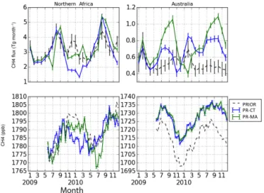
PR-CT and PR-MA yield different CH4 fluxes in
north-ern Africa and Australia (see Fig. 4). We plot these fluxes with the corresponding regional averaged XCH4 values in
Fig. 7. For northern Africa, the difference in XCHproxy4 of up to 10 ppb around January 2010 gives rise to a difference in the monthly posterior flux of 1 Tg month−1. In Australia,
XCHma4 and XCHct4 are in relatively good agreement with each other, with differences within 2 ppb. However, because the a priori fluxes from this region are very small, the differ-ence in the optimized seasonal cycle of fluxes nevertheless becomes relatively large. In particular, PR-MA causes sig-nificant deviations from the a priori fluxes, with decreases in the posterior fluxes during Australian summer, and large increases during winter. Another reason for these flux adjust-ments is the limited land area in the Southern Hemisphere that is available for CH4 flux adjustments (over the open
ocean the a priori flux uncertainties are small, limiting their adjustment).
Detmers et al. (2015) reported an enhanced CO2sink over
central Australia in the second half of 2010 lasting until 2012, caused by an increase in vegetation due to enhanced precipitation during La Niña conditions. If not properly rep-resented in inversions using surface measurements, this neg-ative CO2 anomaly causes XCOmodel2 to be overestimated.
In that case, the anomaly propagates to the proxy retrievals, resulting in overestimation of XCHproxy4 , leading to overes-timated a posteriori CH4fluxes. RATIO estimates a
Figure 7. The top panels show the posterior monthly fluxes inte-grated over TransCom region. Bottom panels show the time series of the mean of XCHproxy4 over northern Africa and Australia. The dotted line in the bottom panels denotes the mean of a priori mod-eled XCH4sampled at GOSAT sites.
(2015) (see Fig. S2 in the Supplement). This results in lower CH4fluxes in the RATIO inversion (see Fig. 4),
demonstrat-ing how the RATIO inversion method can avoid shortcom-ings in the proxy inversions in regions where CO2is poorly
constrained by surface data.
PR-CT and PR-MA have opposite seasonal cycles, which may be due to their XCOmodel2 components that are derived using different ecosystem models. CarbonTracker uses a pri-ori natural fluxes from a CASA simulation driven by actual climatological information, whereas MACC uses only the climatology of natural fluxes. Therefore, the interannual vari-ability of the inverted fluxes in MACC is driven by measure-ments only. Since the surface network does not pose strong constraints on the Australian carbon budget, the differences are driven by the prior fluxes of the two models, which may be more realistic in CarbonTracker in this case.
3.2.5 Aircraft validation
To further investigate the performance of our inversions, we validate the inversion-optimized CH4 and CO2 mixing
ra-tios against independent aircraft measurements obtained dur-ing the projects described in Sect. 2.2. The results of the HIPPO and CONTRAIL validation are shown in Fig. 8 and the values for κ for CH4and the root-mean-square difference
(RMSD) for CO2are given in Fig. 9. κ values are not
calcu-lated for CO2because we do not have the CO2 model
rep-resentation errors used in MACC and CarbonTracker. More details on statistics of the validation are provided in Table S1 in the Supplement.
The difference between HIPPO and PRIOR reflects the overestimated north–south gradient that is found using a pri-ori CH4fluxes, as already discussed in Sect. 3.2.2. In
addi-tion, PRIOR shows a uniform bias of 13.5 ppb. SURF and RATIO correct the north–south gradient and reduce biases to 5.56 and 6.68 ppb, respectively. All the models are per-forming equally well in terms of κ. The original MACC and CarbonTracker CO2 fields have RMSD values of 1.08 and
1.09 ppm, respectively, which is lower than the RMSD of RATIO (1.64 ppm) and SURF (1.65 ppm). We suggest that CarbonTracker and MACC have a better representation of CO2 than PR-CT, PR-MA, and SURF as they assimilate a
larger number of flask measurements sites and also few con-tinuous in situ sites.
Compared with the large CONTRAIL data set of CO2
measurements, only a limited number of CH4measurements
are available, mostly over the Pacific Ocean (see Fig. 1). We observe the same north–south gradient mismatch with PRIOR as seen in the comparison to HIPPO. PR-CT is able to improve the PRIOR κ of 6.99 to 4.56, followed in order of decreasing performance by PR-MA (4.71), SURF (5.33), and RATIO (5.47). The values of κ are larger than 1, which points to significant errors in all the inversion results. The RMSD of the different inversions are comparable. The large data set of CONTRAIL CO2 measurements covers a much
larger area, including flight tracks to Europe and southeast Asia. Our validation shows a mean error of 2.23 ppm in PRIOR. The NOAA and RATIO inversions reduce this bias to −0.43 and −0.41 ppm, respectively. However, similar to the HIPPO validation, MACC (mean bias = −0.2 ppm) and CarbonTracker-derived CO2 (mean bias = 0.11 ppm) fields
are in better agreement with the CONTRAIL measurements than the inversions.
3.2.6 Tropical South America
Tropical South America contains the Amazon Basin, which is a large reservoir of standing biomass and contains one of the largest wetlands in the world. Therefore, it plays an im-portant role in the annual global budget of both CO2 and
CH4. Inversion results for the region have been validated
using AMAZONICA measurements (see Fig. S5 and Ta-ble S1 in the Supplement). Generally, the model results us-ing PRIOR fluxes underestimate the measured CH4
mix-ing ratios (mean offset = −32.02 ppb). All inversions correct this offset, with SURF performing best (mean mismatch =
−14.18 ppb). RATIO closely follows SURF with a mean mismatch of −17.18 ppb. The proxy inversions have a higher mismatch than RATIO and SURF, with means of −20.30 and
−24.11 ppb, respectively for PR-MA and PR-CT. The κ val-ues for the AMAZONICA CH4 measurements (see Fig. 9)
again show that fluxes from RATIO lead to lower mismatches than those from PR-CT and PR-MA. RATIO predicts this region as a significantly high CH4 source for the first half
of 2010 (see Fig. 4), and is in good agreement with aircraft measurements.
To check whether this is caused by errors in XCOmodel2 , we perform similar comparisons using AMAZONICA CO2
Figure 8. Validation of inversion-optimized concentration fields of CO2and CH4with airborne measurements.
Figure 9. Summary of aircraft validation results per project for CH4
(a, expressed as κ) and CO2(b, expressed as RMSD) for the whole
inversion time period i.e., from 1 January 2009 to 31 December 2010.
measurements. We find that the two original models repre-sent CO2about equally well in terms of RMSD (see Table S1
in the Supplement). Therefore, the higher mismatch of PR-CT and PR-MA for CH4is not due to a poor representation
of the XCOmodel2 over the region. This raises the question as to why RATIO performs better. In Sect. 3.1, we observe that the error in COmodel2 is generally lower than the error in the GOSAT Xratioretrievals. In proxy inversions, this retrieval
er-ror, which is coming from Xratio(see Eq. 2), is directly
trans-ferred to CH4fluxes, whereas in RATIO it is distributed over
the CH4and CO2part of the state vector. The high posterior
CO2flux uncertainties for RATIO in the region support this
further (see Fig. 5).
Flux maps of the region show that the satellite inver-sions provide a more spatially resolved adjustment of the CH4 fluxes than SURF (see Fig. S3 in the Supplement).
The satellite inversions estimate higher fluxes in the north-west corner of the region near Colombia. Similar increases have been reported in earlier studies, assimilating satellite-retrieved XCH4 (Monteil et al., 2013; Frankenberg et al.,
2006). The spatial pattern of the flux adjustment suggests that the proxy inversions compensate the increase over Colom-bia by reducing the fluxes in the Amazon Basin, which is less well covered by satellite retrievals due to frequent cloud cover. This may explain why the proxy inversions end up underestimating the observations inside the basin. SURF is mainly constrained by the large-scale inter-hemispheric gra-dient. This leads to a different pattern of flux adjustments, increasing only the fluxes in the southern part of the region while keeping the fluxes in Amazon Basin close to the prior. This solution brings SURF in relatively close agreement with the measurements. RATIO also shows a flux enhancement in Colombia, but at the same time represents the Amazon Basin better than the proxy inversions, likely because of its larger number of degrees of freedom in modifying regional flux pat-terns of both CO2and CH4.
Gatti et al. (2014) and Van der Laan et al. (2015) reported an anomalous natural source of CO2in the region in 2010,
study, RATIO predicts a more enhanced CO2natural source
than the SURF and PRIOR. RATIO (RMSD = 3.23 ppm) is also in better agreement in terms of RMSD with AMAZON-ICA CO2data than SURF (RMSD = 3.31 ppm) and PRIOR
(3.38 ppm). This demonstrates, like in the case of Australia, that the RATIO method is capable of informing us about the CO2fluxes, from which the CH4 flux estimation
bene-fits also.
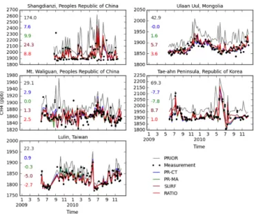
3.2.7 Temperate Eurasia
As mentioned in Sect. 3.2.2, SURF leads to a drastic flux re-duction in temperate Eurasia, whereas all satellite inversions show comparatively smaller decreases. Here, we investigate this in further detail by analyzing the inversion-optimized fits to the NOAA measurements at five surface sites located in this region (see Fig. 10). We find large mismatches between the a priori simulated concentrations and the measurement at these sites, with mean offsets ranging between 29.1 ppb at Mt. Waliguan and 174 ppb at Shangdianzi. All inversions correct for this mismatch by decreasing the regional fluxes. Surprisingly enough, the satellite inversions are able to fit the flask measurements even better than SURF, despite smaller corrections to the fluxes. For example, the mean posterior mismatch at Shangdianzi is 24.3 ppb for SURF, and only 7.5 to 9.8 ppb for the satellite inversions. A possible expla-nation is the double counting of surface data in the satel-lite inversions, as the satelsatel-lite data have been bias corrected using an inversion that was already optimized using surface data. However, the bias correction is only applied as a zonal and annual mean. All inversions show similar reductions in the fluxes from eastern temperate Eurasia (mostly China) to match the NOAA measurements. However, the satellite in-versions tend to compensate for this flux decrease over China by increased fluxes in India and the central part of temperate Eurasia.
4 Discussion
We have demonstrated that the application of the ratio method to GOSAT data yields realistic solutions for CO2and
CH4fluxes. Its performance is comparable, and may in some
regions even be better than the proxy inversion method. This is an important finding because the Xratioretrieval approach
provides a useful alternative to the full-physics method in that cloud filtering is less critical. In the case of GOSAT, it increases the number of useful measurements by about a fac-tor of 2 (Butz et al., 2010; Fraser et al., 2014). At the same time, the RATIO inversion method avoids using the model-derived CO2fields as a hard constraint, which is an important
limitation of the proxy method.
The realistic performance of the ratio method is certainly not a trivial outcome, since it prompts the user for specifica-tion of new uncertainties, influencing the way in which
mea-Figure 10. Inversion-optimized fits to surface measurement sites in temperate Eurasia. The numbers in the plots are the mean biases of models with measurements.
surement information is shared between CH4and CO2. The
joint CO2 and CH4 inversion problem has a larger number
of degrees of freedom, as a result of which CH4flux
adjust-ments can compensate for errors in CO2and vice versa.
As-similating surface measurements helps to decouple CH4and
CO2, which works best in regions that are relatively well
cov-ered by the surface network.
In other regions, the method can be improved further by accounting for correlations between a priori fluxes of CH4
and CO2. This study does not specify such correlations,
which correspond to the assumption that a priori CO2 and
CH4flux uncertainties are independent of each other. Fraser
et al. (2014) accounted for a priori uncertainty correlations for biomass burning fluxes of CO2 and CH4, based on the
available information about emission ratios. Imposing such a priori constraints increased posterior uncertainty reduction compared to other methods for both CH4and CO2in some
regions.
It is noteworthy that the inversions are run assuming un-correlated measurements and a perfect transport. Also, as we are not optimizing the atmospheric sink of CH4, all the
infor-mation from its budget is used to constrain the surface fluxes. Hence, the estimates of posterior uncertainties tend to be op-timistic in this study. The χ2 statistic indicates whether the assumed measurement and prior errors are statistically con-sistent (Meirink et al., 2008). We find χ2/ns=0.93 for RA-TIO, 0.96 for PR-CT, 0.93 for PR-LM, and 1.14 for SURF in the CH4inversions (ns is the number of observations as-similated in the inversion). This shows that we are not dras-tically underestimating the prior uncertainties in our CH4
One problem with the ratio method is the assimilation of Xratio over oceans. The uncertainty of CH4 fluxes over the
open oceans is relatively small. As a result, the model–data mismatch over the ocean is mostly accounted for by adjust-ing the CO2fluxes, which has a larger a priori uncertainty. At
the same time, CO2fluxes over oceans tend to be very
sensi-tive to small and systematic model–data mismatches of a few tenths of a ppm (Basu et al., 2013). Any bias in atmospheric transport, affecting both CO2 and CH4, is projected on the
CO2 fluxes, which may lead to rather unrealistic estimates
of the annual CO2 exchange over oceanic regions. Palmer
et al. (2006) proposed to account for cross correlations in the model representation error between the components of a dual tracer inversion, which could reduce the extent of this prob-lem.
Our surface-only inversion shows a large decrease in the fluxes from temperature Eurasia. To better understand this, we look at results of other recently published CH4inversion
results. We group the studies into three groups: (1) studies not using EDGAR v4.2 as a priori fluxes, comprising Houwel-ing et al. (2014), Monteil et al. (2013), Bruhwiler et al. (2014), and Fraser et al. (2013); (2) studies using EDGAR v4.2 but not assimilating the Shangdianzi site, comprising Alexe et al. (2015) and Bergamaschi et al. (2013); (3) stud-ies using EDGAR v4.2 and assimilating Shangdianzi site comprising this work and Thompson et al. (2015). The in-versions of group 1 do not show a systematic reduction in fluxes of temperate Eurasia. Inversions of group 3 tend to re-duce the fluxes from the region the most; whereas, group 2 reduces fluxes by an intermediate amount. This outcome is partly explained by the EDGAR 4.2 fluxes being substan-tially higher in temperate Eurasia than previous EDGAR ver-sions, as found also by Bergamaschi et al. (2013). In ad-dition, however, these increased fluxes have the largest im-pact on surface-only inversions assimilating measurements from the Shangdianzi site, possibly due to a nearby hotspot in EDGAR v4.2. The hotspot is located near Jiexiu in the Shanxi province (112◦E, 37◦N), and has coal emissions of 10.83 Tg y−1for the year 2010 from a 10 × 10 km grid. Ac-cording to the EDGAR team (G. Meanhout, personal com-munication, 2015), this unrealistically high local source of CH4 is the consequence of disaggregating large emission
from Chinese coal mining using the limited available infor-mation on the location of the coal mines. Thompson et al. (2015), the other study in group 3, show a large a pri-ori mismatch with a root-mean-square error of 103 ppb at Shangdianzi. Their inversions reduce their a priori east Asian CH4 fluxes of 82 Tg y−1 by 23 Tg y−1, with large
adjust-ments in the fluxes from rice cultivation. Further research is needed to investigate the implications of the shortcom-ings of EDGAR v4.2. It is noteworthy, however, that when satellite data are assimilated in these studies, the improved regional coverage reduces the impact of this local disaggre-gation problem on the estimated regional fluxes.
5 Conclusions
This study investigated the use of GOSAT-retrieved Xratiofor
constraining the surface fluxes of CO2 and CH4. First, we
validated the XCH4, XCO2, and Xratioretrievals, as well as
the model-derived XCO2fields used in the proxy methods,
using TCCON measurements. This analysis confirmed that biases in non-scattering XCH4 and XCO2retrievals largely
cancel out in Xratio. Xratiohas a larger mean bias than
model-derived XCO2from CarbonTracker and MACC, suggesting
that mostly retrieval biases, rather than CO2 model errors,
limit the performance of the proxy method. This is true, es-pecially at a large temporal and spatial scale. To account for biases in GOSAT-retrieved Xratio, a TCCON-derived
correc-tion was applied as a funccorrec-tion of surface albedo, resulting in a mean adjustment of −0.74 %. An additional correction was applied to Xratio, XCHct4, and XCHma4 to account for a bias
between NOAA-optimized CH4fields in TM5 and
TCCON-observed XCH4, amounting to −0.76, −0.80, and 0.59 %,
respectively.
We optimized monthly CH4 and CO2fluxes for the year
2009 and 2010 by assimilating GOSAT-retrieved Xratiodata
using the TM5–4DVAR inverse modeling system. Additional inversions, assimilating XCHproxy4 and NOAA surface flask measurements, were performed in a similar setup for com-parison. The posterior uncertainties of the fluxes are calcu-lated with a Monte Carlo approach.
Overall, the ratio and proxy inversions show similar re-sults for annual CH4fluxes. Significant seasonal differences
in CH4 are found between the two proxy inversions for
TransCom regions northern Africa and Australia, which can be traced back to differences in XCOmodel2 . The CO2models
show a systematic difference in the seasonal cycle of CO2,
resulting in a seasonally varying mismatch in the northern tropics. The ratio method has the advantage that it allows adjustment of the CO2fluxes, whereas the proxy inversions
can only account for this mismatch by adjusting CH4. For
Australia, the proxy inversions predict an anomalous CH4
increase in the second half of 2010. This difference can be explained by errors in XCOmodel2 , which does not account for the anomalous carbon sink reported by Detmers et al. (2015) for lack of surface measurement coverage. The ratio method has the built-in flexibility needed to attribute the anomaly to CO2instead of CH4, and is therefore is not affected.
Inversions using satellite data show a better agreement among each other compared to the NOAA-only inversions, which use only surface data. This is true in particular for temperate Eurasia, where the NOAA-only inversion reduces the annual CH4 flux by as much as 55 Tg y−1, relative to
an a priori flux of 121 Tg y−1. This is traced back to a large overestimation of atmospheric CH4 concentration in
the prior model at NOAA sites in the region, especially at Shangdianzi, where the prior model overestimates the data by 179 ppb on average. When satellite measurements are as-similated, the CH4 flux reduction for temperate Eurasia is
limited to 21 Tg y−1, while accounting for the a priori
mis-match in Shangdianzi.
We validated the inversion-optimized atmospheric tracer fields, as well as the CarbonTracker and MACC CO2 fields
used in the proxy inversions, against three independent air-craft measurement projects. For CH4, the ratio and
NOAA-only inversions showed a lower mismatch with HIPPO and AMAZONICA measurements than the two proxy inversions. Further analysis shows that this is not due to a better repre-sentation of atmospheric CO2 in the ratio inversion.
How-ever, the ratio inversion accounts for inconsistent constraints from Xratioby correcting both CH4and CO2fluxes, whereas
the proxy inversions can only attribute such constraints to CH4 fluxes. The ratio inversion predicts an enhanced CO2
natural source in this region during 2010 compared with the NOAA-only and a priori model. This is in accordance with the findings of Gatti et al. (2014) and Van der Laan
et al. (2015), and is also supported by the AMAZONICA aircraft measurements. Overall, this study shows that the ra-tio method is capable of informing us about surface fluxes of CH4and CO2using satellite measurements, and that it
pro-vides a useful alternative for the proxy inversion method.
Data availability
Level 2 XCH4and Xratiodata from GOSAT/TANSO are
cal-culated using the RemoTeC algorithm. The data are publicly available from the ESA’s Climate Change Initiative website (http://www.esa-ghg-cci.org/). NOAA’s GGGRN CH4
mea-surements are publically available at ftp://aftp.cmdl.noaa. gov/data/trace_gases/ch4/flask/surface/. CarbonTracker CO2
fluxes are provided by NOAA ESRL, Boulder, Colorado, USA from the website at http://carbontracker.noaa.gov.
Appendix A: Bias correction
We apply a two-step correction to reduce the influence of biases in our inversions.
1. TCCON-based: residual biases in Xratio remain that
are not accounted for by calculating the ratio between XCHns4 and XCOns2. The standard bias correction proce-dure in the RemoTeC XCHproxy4 retrieval assumes a lin-ear dependence on surface albedo (Guerlet et al., 2013). However, this procedure would also correct biases in XCOmodel2 , which are not expected to vary with surface albedo. Therefore, we apply the albedo-based bias cor-rection only to the GOSAT-measured Xratio. To
deter-mine the bias correction, we use GOSAT retrievals that are co-located with TCCON measurements; i.e., they are within 5◦ latitude and longitude and within 2 h of TCCON measurements. The relationship between sur-face albedo at 1593 nm and the monthly difference be-tween GOSAT and TCCON is shown in Fig. A1. A global bias correction function, obtained by linear re-gression, results in a mean adjustment of −0.74 % of GOSAT Xratio.
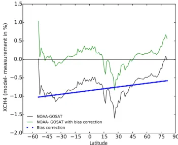
2. NOAA-based: a systematic mismatch between the NOAA and GOSAT-optimized TM5 CH4 fields has
been discussed in Monteil et al. (2013). The cause of this problem is still unresolved, but may be explained in part by transport model uncertainties in representing XCH4 in the stratosphere. Several other studies have
reported similar biases and applied NOAA-based bias corrections, in addition to the TCCON-derived retrieval corrections in order to restore consistency between the observational constraints provided by surface and to-tal column measurements (Alexe et al., 2015; Houwel-ing et al., 2014; Basu et al., 2013). We use a simi-lar procedure for Xratio and XCHproxy4 data by
com-paring the TCCON-corrected GOSAT retrievals to the NOAA-optimized TM5 model. The mean difference is corrected using a linear function of latitude. This results in a mean adjustment of −0.76 % in Xratio, −0.59 % in
XCHma4 , and −0.80 % in XCHct4 (see Figs. A2 and A3).
Figure A1. Linear regression analysis between GOSAT–TCCON Xratioand surface albedo at 1593 nm.
60 45 30 15 0 15 30 45 60 75 90
Latitude2.0
1.5
1.0
0.5
0.0
0.5
1.0
1.5
XCH4 (model- measurement in %)
NOAA-GOSATNOAA- GOSAT with bias correction Bias correction
Figure A2. NOAA-based bias correction applied to XCH4in the
PR-CT inversion.
60 45 30 15 0 15 30 45 60 75 90
Latitude1.5
1.0
0.5
0.0
0.5
1.0
XCH4 (model- measurement in %)
NOAA-GOSATNOAA- GOSAT with bias correction Bias correction
Figure A3. NOAA-based bias correction applied to Xratio in the
Appendix B: Posterior uncertainty
As discussed in Pandey et al. (2015), the Xratio inversion
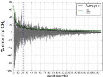
problem is weakly nonlinear and is solved using the quasi-Newtonian optimizer M1QN3. The standard implementation of M1QN3 does not provide an estimate of posterior uncer-tainties. Therefore, we use the Monte Carlo approach as de-scribed in Chevallier et al. (2007) to calculate posterior flux uncertainties. For the linear SURF and proxy inversions, we use the conjugate gradient optimization method. The poste-rior flux uncertainties of these inversions are derived using the same approach to keep the comparison between the un-certainties consistent. A sensitivity test has been performed to determine the size of the ensemble needed to properly cap-ture the 1σ of the prior fluxes. Figure B1 shows the results of this experiment. We choose an ensemble size of 24 for our experiments, which gives a 1σ estimate with 14.4 % uncer-tainty.
Figure B1. The gray lines represent the percentage error of 1σ of ensemble size n from the σ of ensemble size of 200 of the a pri-ori CH4 flux integrated over TransCom regions. The dark black
line represents the average deviation in the gray lines. The green line represents the analytical variation of the error of 1σ (Bousserez et al., 2015). A constant difference of approx. 6 % between the esti-mates comes from the finite size of the largest sample (200).
The Supplement related to this article is available online at doi:10.5194/acp-16-5043-2016-supplement.
Acknowledgements. This work is supported by the Netherlands Organization for Scientific Research (NWO), project number ALW-GO-AO/11-24. The computations were carried out on the Dutch national supercomputer Cartesius, and we thank SURFSara (www.surfsara.nl) for their support. Access to the GOSAT data was granted through the third GOSAT research announcement jointly issued by JAVA, NIES, and MOE. The funding for AMAZONICA project is provided by NERC and FAPESP. We thank S. C. Wofsy for providing HIPPO data. We thank Debra Wunch and other TCCON principal investigators for making their measurements available.
Edited by: A. Stohl
References
Alexe, M., Bergamaschi, P., Segers, A., Detmers, R., Butz, A., Hasekamp, O., Guerlet, S., Parker, R., Boesch, H., Frankenberg, C., Scheepmaker, R. A., Dlugokencky, E., Sweeney, C., Wofsy, S. C., and Kort, E. A.: Inverse modelling of CH4 emissions for 2010–2011 using different satellite retrieval products from GOSAT and SCIAMACHY, Atmos. Chem. Phys., 15, 113–133, doi:10.5194/acp-15-113-2015, 2015.
Basu, S., Guerlet, S., Butz, A., Houweling, S., Hasekamp, O., Aben, I., Krummel, P., Steele, P., Langenfelds, R., Torn, M., Biraud, S., Stephens, B., Andrews, A., and Worthy, D.: Global CO2
fluxes estimated from GOSAT retrievals of total column CO2, Atmos. Chem. Phys., 13, 8695–8717, doi:10.5194/acp-13-8695-2013, 2013.
Basu, S., Krol, M., Butz, A., Clerbaux, C., Sawa, Y., Machida, T., Matsueda, H., Frankenberg, C., Hasekamp, O., and Aben, I.: The seasonal variation of the CO2flux over Tropical Asia estimated
from GOSAT, CONTRAIL, and IASI, Geophys. Res. Lett., 41, 1809–1815, doi:10.1002/2013GL059105, 2014.
Bergamaschi, P., Frankenberg, C., Meirink, J. F., Krol, M., Den-tener, F., Wagner, T., Platt, U., Kaplan, J. O., Körner, S., Heimann, M., Dlugokencky, E. J., and Goede, A.: Satellite char-tography of atmospheric methane from SCIAMACHY on board ENVISAT: 2. Evaluation based on inverse model simulations, J. Geophys. Res., 112, D02304, doi:10.1029/2006JD007268, 2007. Bergamaschi, P., Krol, M., Meirink, J. F., Dentener, F., Segers, A., van Aardenne, J., Monni, S., Vermeulen, A. T., Schmidt, M., Ramonet, M., Yver, C., Meinhardt, F., Nisbet, E. G., Fisher, R. E., O’Doherty, S., and Dlugokencky, E. J.: Inverse modeling of European CH4emissions 2001–2006, J. Geophys. Res., 115, D22309, doi:10.1029/2010JD014180, 2010.
Bergamaschi, P., Houweling, S., Segers, A., Krol, M., Frankenberg, C., Scheepmaker, R. A., Dlugokencky, E., Wofsy, S. C., Kort, E. A., Sweeney, C., Schuck, T., Brenninkmeijer, C., Chen, H., Beck, V., and Gerbig, C.: Atmospheric CH4in the first decade of
the 21st century: Inverse modeling analysis using SCIAMACHY satellite retrievals and NOAA surface measurements, J. Geophys. Res.-Atmos., 118, 7350–7369, doi:10.1002/jgrd.50480, 2013.
Bousquet, P., Ciais, P., Miller, J. B., Dlugokencky, E. J., Hauglus-taine, D. A., Prigent, C., Van der Werf, G. R., Peylin, P., Brunke, E.-G., Carouge, C., Langenfelds, R. L., Lathière, J., Papa, F., Ramonet, M., Schmidt, M., Steele, L. P., Tyler, S. C., and White, J.: Contribution of anthropogenic and natural sources to atmospheric methane variability, Nature, 443, 439–43, doi:10.1038/nature05132, 2006.
Bousserez, N., Henze, D. K., Perkins, A., Bowman, K. W., Lee, M., Liu, J., Deng, F., and Jones, D. B. A.: Improved analysis-error covariance matrix for high-dimensional variational inver-sions: application to source estimation using a 3D atmospheric transport model, Q. J. Roy. Meteor. Soc., 141, 1906–1921, doi:10.1002/qj.2495, 2015.
Bruhwiler, L., Dlugokencky, E., Masarie, K., Ishizawa, M., An-drews, A., Miller, J., Sweeney, C., Tans, P., and Worthy, D.: CarbonTracker-CH4: an assimilation system for estimating
emis-sions of atmospheric methane, Atmos. Chem. Phys., 14, 8269– 8293, doi:10.5194/acp-14-8269-2014, 2014.
Butz, A., Hasekamp, O. P., Frankenberg, C., Vidot, J., and Aben, I.: CH4 retrievals from space-based solar backscatter
mea-surements: Performance evaluation against simulated aerosol and cirrus loaded scenes, J. Geophys. Res., 115, D24302, doi:10.1029/2010JD014514, 2010.
Butz, A., Guerlet, S., and Hasekamp, O.: Toward accurate CO2
and CH4 observations from GOSAT, Geophys. Res. Lett., 38,
L14812, doi:10.1029/2011GL047888, 2011.
Chevallier, F.: On the parallelization of atmospheric inversions of CO2 surface fluxes within a variational framework, Geosci. Model Dev., 6, 783–790, doi:10.5194/gmd-6-783-2013, 2013. Chevallier, F., Bréon, F.-M., and Rayner, P. J.: Contribution
of the Orbiting Carbon Observatory to the estimation of CO2 sources and sinks: Theoretical study in a variational
data assimilation framework, J. Geophys. Res., 112, D09307, doi:10.1029/2006JD007375, 2007.
Chevallier, F., Ciais, P., Conway, T. J., Aalto, T., Anderson, B. E., Bousquet, P., Brunke, E. G., Ciattaglia, L., Esaki, Y., Fröhlich, M., Gomez, A., Gomez-Pelaez, A. J., Haszpra, L., Krummel, P. B., Langenfelds, R. L., Leuenberger, M., Machida, T., Maig-nan, F., Matsueda, H., Morguí, J. A., Mukai, H., Nakazawa, T., Peylin, P., Ramonet, M., Rivier, L., Sawa, Y., Schmidt, M., Steele, L. P., Vay, S. A., Vermeulen, A. T., Wofsy, S., and Wor-thy, D.: CO2surface fluxes at grid point scale estimated from a global 21 year reanalysis of atmospheric measurements, J. Geo-phys. Res., 115, D21307, doi:10.1029/2010JD013887, 2010. Chevallier, F., Palmer, P., Feng, L., Boesch, H., O’Dell, C.,
and Bousquet, P.: Toward robust and consistent regional CO2
flux estimates from in situ and spaceborne measurements of atmospheric CO2, Geophys. Res. Lett., 41, 1065–1070,
doi:10.1002/2013GL058772, 2014.
Dee, D. P., Uppala, S. M., Simmons, A. J., Berrisford, P., Poli, P., Kobayashi, S., Andrae, U., Balmaseda, M. A., Balsamo, G., Bauer, P., Bechtold, P., Beljaars, A. C. M., van de Berg, L., Bid-lot, J., Bormann, N., Delsol, C., Dragani, R., Fuentes, M., Geer, A. J., Haimberger, L., Healy, S. B., Hersbach, H., Hólm, E. V., Isaksen, L., Kållberg, P., Köhler, M., Matricardi, M., McNally, A. P., Monge-Sanz, B. M., Morcrette, J.-J., Park, B.-K., Peubey, C., de Rosnay, P., Tavolato, C., Thépaut, J.-N., and Vitart, F.: The ERA-Interim reanalysis: configuration and performance of the