HAL Id: hal-01017853
https://hal.archives-ouvertes.fr/hal-01017853v2
Submitted on 16 Sep 2014
HAL is a multi-disciplinary open access
archive for the deposit and dissemination of
sci-entific research documents, whether they are
pub-lished or not. The documents may come from
teaching and research institutions in France or
abroad, or from public or private research centers.
L’archive ouverte pluridisciplinaire HAL, est
destinée au dépôt et à la diffusion de documents
scientifiques de niveau recherche, publiés ou non,
émanant des établissements d’enseignement et de
recherche français ou étrangers, des laboratoires
publics ou privés.
Anomaly Detection Based on Aggregation of Indicators
Tsirizo Rabenoro, Jérôme Lacaille, Marie Cottrell, Fabrice Rossi
To cite this version:
Tsirizo Rabenoro, Jérôme Lacaille, Marie Cottrell, Fabrice Rossi. Anomaly Detection Based on
Aggre-gation of Indicators. 23rd annual Belgian-Dutch Conference on Machine Learning (Benelearn 2014),
Jun 2014, Bruxelles, Belgium. pp.64-71. �hal-01017853v2�
Tsirizo Rabenoro [email protected]
J´erˆome Lacaille [email protected]
Health Monitoring Department, Snecma, Safran Group, Moissy Cramayel, France
Marie Cottrell [email protected]
Fabrice Rossi [email protected]
SAMM (EA 4543), Universit´e Paris 1, Paris, France
Keywords: Anomaly Detection, Turbofan, Health Monitoring
Abstract
Automatic anomaly detection is a major issue in various areas. Beyond mere detection, the identification of the origin of the problem that produced the anomaly is also essential. This paper introduces a general methodol-ogy that can assist human operators who aim at classifying monitoring signals. The main idea is to leverage expert knowledge by generating a very large number of indicators. A feature selection method is used to keep only the most discriminant indicators which are used as inputs of a Naive Bayes classifier. The parameters of the classifier have been optimized indirectly by the selection process. Simulated data designed to reproduce some of the anomaly types observed in real world engines.
1. Introduction
Automatic anomaly detection is a major issue in numer-ous areas and has generated a vast scientific literature (Chandola et al., 2009). Among the possible choices, statistical techniques for anomaly detection are appeal-ing because they can make use of expert knowledge about the expected normal behaviour of the studied system. Thus they can compensate for the limited availability of faulty observations (or more generally of labelled observations). Those techniques are generally based on a stationarity hypothesis. Numerous paramet-ric and nonparametparamet-ric methods have been proposed to
Appearing in Proceedings of BENELEARN 2014. Copyright 2014 by the author(s)/owner(s).
achieve this goal (Basseville & Nikiforov, 1995). However, statistical tests efficiency is highly dependent on the adequacy between the assumed and actual data distribution. In addition, statistical methods rely on meta-parameters, such as the length of the time window on which a change is looked for. These meta-parameters have to be tuned to give maximal efficiency.
This article proposes to combine a (supervised) classi-fication approach to statistical techniques in order to obtain an automated anomaly detection system that leverages both expert knowledge and labelled data sets. The main idea consists in building a large number of binary indicators that correspond to anomaly detection decisions taken by statistical tests suggested by the ex-perts, with varying (meta)-parameters. Then a feature selection method is applied to the high dimensional binary vectors to select the most discriminative ones, using a labelled data set. Finally, a classifier is trained on the reduced binary vectors to provide automatic detection for future samples.
This approach has numerous advantages. On the classi-fication point of view, it has been shown in e.g. (Fleuret, 2004) that selecting relevant binary features among a large number of simple features can lead to very high classification accuracy in complex tasks. In addition, using features designed by experts allows one to at least partially interpret the way the classifier is making decisions as none of the features will be of a black box nature. This is particularly important in aircraft engine health monitoring context (see Section 2). The indicators play also a homogenisation role by hiding the complexity of the signals (in a way similar to the one used in (Hegedus et al., 2011), for instance). On the statistical point of view, the proposed approach brings a form of automated tuning: a test recommended by
Anomaly Detection
an expert can be included in numerous variants. The feature selection process keeps the most adapted pa-rameters.
The rest of the paper is organized as follows. Section 2 describes in more details Snecma’s engine health monitoring context which motivates this study. Section 3 presents in more details the proposed methodology. Section 4 presents the results obtained on simulated data.
2. Application context
2.1. Introduction and Objectives
To improve the already high availability rate of aircraft engine, health monitoring is developed. This process consists in ground based monitoring of numerous mea-surements made on the engine and its environment during the aircraft operation.
One of the goals of this monitoring is to detect abnormal behaviour of the engine that are early signs of potential failures. This detection is done through the analysis of data coming from sensors embedded in the engine. Flight after flight, measurements, such as exhausted gas temperature (EGT) and high pressure (HP) core speed (N2) form a time series.
On one hand, missing such an early sign can lead to operational events such as in flight shut down. Such operational events can cause high maintenance costs. On the other hand, a false alarm (detecting an anomaly when the engine is behaving normally) can have also costly consequences such as useless engine removal procedure.
Thus to minimize false alarm, each potential anomaly has to be confirmed by a human operator. He is then in charge of the identification of the origin of the anomaly. The long term goal of engine manufacturers is to help companies to minimize their maintenance costs by giv-ing maintenance recommendations as accurate as pos-sible. Human operators have a very important role in the current industrial process: the goal is to help them make improved decisions thanks to a grey box classifier, mainly because the complexity of the problem seems to prevent any fully automated decision making. The methodology introduced in this paper aims at help-ing human operators by leveraghelp-ing expert knowledge and relying on feature selection to keep only a small number of binary indicators.
2.2. Health monitoring
Monitoring is strongly based on experts knowledge and field experience. Faults and early signs of failures are identified from suitable measurements associated to adapted computational transformations of the data. We refer the reader to e.g. (Rabenoro & Lacaille, 2013) for examples of the types of measurements and transformations that can be used in practice.
One of the main difficulties faced by the experts consists in removing from the measurements any dependency from the flight context. This normalization process is extremely important as it allows one to assume station-arity of the residual signal and therefore to leverage change detection methods. In practice, experts build some anomaly score from those stationarity hypotheses and when the score passes a limit, the corresponding early sign of failure is signalled to the human operator. See (Cˆome et al., 2010), (Flandrois et al., 2009) and (Lacaille, 2009) for some examples.
One of the problems induced by this general approach is that experts are generally specialized on a particular subsystem, thus each anomaly score is mainly focused on a particular subsystem despite the need of a diag-nostic of the whole system. This task is done by human operator who collects all available information about the desired engine. One of the benefits of the proposed methodology is its ability to handle binary indicators coming from all subsystems in an integrated way, as explained in the next section.
3. Methodology
The suggested methodology is based on the selection and combination of a large number of binary indicators. While this idea is not entirely new (see e.g., (Fleuret, 2004; Hegedus et al., 2011)), the methodology proposed here has some specific aspects. Rather than relying on very basic detectors as in (Fleuret, 2004) or on fixed high level expertly designed ones as in (Hegedus et al., 2011), our method takes an intermediate approach: it varies the parameters of a set of expertly designed para-metric indicators. In addition, it aims at providing an interpretable model. This section details the proposed procedure.
3.1. Expert knowledge
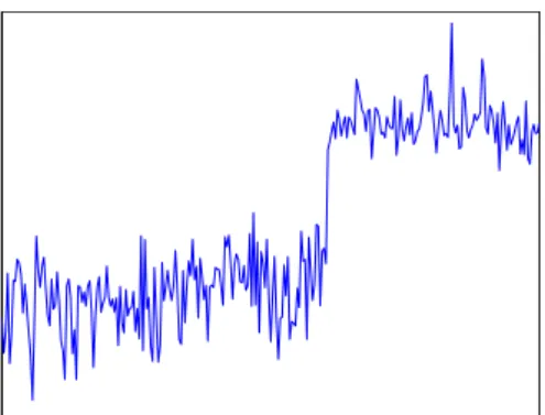
This article focuses on change detection based on sta-tistical techniques (Basseville & Nikiforov, 1995). In many contexts, experts can generally describe more or less explicitly the type of change they are expecting for some specific (early signs of) anomalies. In the pro-posed application context, one can observe for instance
a mean shift as in Figure 1.
Figure 1. Mean shift in a real world time series.
More generally, experts can describe aggregation and transformation techniques of raw signals that lead to quantities which should behave in a “reasonable man-ner” under normal circumstances. This can in general be summarized by computing a distance between the actual quantities and their expected values.
3.2. Exploring parameters space
In practice however, experts can seldom provide de-tailed parameter settings for the aggregation and trans-formation techniques they recommend. Fixing the threshold above which a distance from the “reasonable values” becomes critical is also difficult.
Let us consider for illustration purposes that the expert recommends to look for shifts in mean of a certain quantity as early signs of a specific anomaly (as in Figure 1). If the expert has no strong prior on the distribution of the quantity, a usual test would be the Mann-Whitney U test.
Then, one has to assess the scale of the shift. The expert has to specify the length of time windows (that defines the scale at which the shift may appear) of the two compared populations. In most cases, the experts can only give a rough idea of the scale.
Given the choice of the test, of its scale and of a change point, to take a decision, one has to choose a level to which the p-value will be compared.
So all in one, looking for a mean shift can be done by choosing at least three parameters: the type of the test, the scale at which the shift can occur and the level of the test. The methodology consists in considering (a subset of) all possible combinations of parameters compatible with expert knowledge to generate binary indicators. This is a form of indirect grid search procedures for meta-parameter optimisation.
3.3. Confirmation indicators
Finally, aircraft engines are extremely reliable, a fact that increases the difficulty in balancing sensibility and specificity of anomaly detectors. High level confirma-tion indicators are built from low level tests to alleviate this difficulty. For instance, if we monitor the evolu-tion of a quantity on a long period compared to the expected time scale of anomalies, we can compare the number of times the null hypothesis of a test has been rejected on the long period with the number of times it was not rejected, and turn this into a binary indicator with a majority rule.
3.4. Decision
To summarize, we construct parametric anomaly scores from expert knowledge, together with acceptable pa-rameter ranges. By exploring those ranges, we gener-ate numerous (possibly hundreds of) binary indicators. Each indicator can be linked to an expertly designed score with a specific set of parameters and thus is sup-posedly easy to interpret by operators. Notice that while we focused in this presentation on temporal data, this framework can be applied to any data source. The final decision step consists in classifying these high dimensional binary vectors in order to further discrimi-nate between seriousness of anomalies and/or sources (in terms of subsystems of the engine, for instance). While including hundreds of indicators is important to give a broad coverage of the parameters space of the expert scores, it seems obvious that some redundancy will appear. Moreover reduce the number of indicators will ease the interpretation by limiting the quantity of informations transmitted to the human operator. Thus feature selection (Guyon & Elisseeff, 2003) is ap-propriate. Unlike (Hegedus et al., 2011) who choose features by random projection, the proposed methodol-ogy favours interpretable solutions, even at the expense of the classification accuracy: the goal is to help the human operator, not to replace her/him. Among the possible solutions, we choose to use the Mutual infor-mation based technique Minimum Redundancy Max-imum Relevance (mRMR, (Peng et al., 2005)) which was reported to give excellent results on high dimen-sional data (see also (Fleuret, 2004) for another possible choice).
In the considered context, black box modelling is not acceptable, so while numerous classification algorithms are available (see e.g. (Kotsiantis et al., 2007)), we shall focus on interpretable ones. Random Forests (Breiman, 2001) are chosen as the reference method as they are very adapted to high dimensional data and known to
Anomaly Detection
be robust and to provide state-of-the-art classification performances. While they are not as interpretable as their ancestors CART (Breiman et al., 1984), they provide at least variable importance measures that can be used to identify the most important indicators. Another classification algorithm used in this paper is Naive Bayes classifier (Koller & Friedman, 2009) which is also appropriate for high dimensional data. They are known to provide good results despite the strong assumption of the independence of features given the class. In addition, decisions taken by a Naive Bayes classifier are very easy to understand thanks to the estimation of the conditional probabilities of the feature in each class. Those quantities can be shown to the human operator as references.
4. Experiments
The proposed methodology is evaluated on simulated data which have been modelled based on real world data such as the ones shown on Figure 1.
4.1. Simulated data
We consider univariate time series of variable length in which three types of shifts can happen: the mean shift described in Section 3.1, together with a variance and a trend shift described below. Two data sets are generated, A and B.
In both cases, it is assumed that expert based normal-ization has been performed. Therefore when no shift in the data distribution occurs, we observe a station-ary random noise modelled by the standard Gaussian distribution, that is n random variables X1, . . . , Xn
independent and identically distributed according to N (µ = 0, σ2
= 1). Signals have a length chosen uni-formly at random between 100 and 200 observations The three types of shift are :
1. a variance shift: in this case, observations are distributed according to N (µ = 0, σ2
) with σ2
= 1 before the change point and σ chosen uniformly at random in [1.01, 5] after the change point; 2. a mean shift: in this case, observations are
dis-tributed according to N (µ, σ2
= 1) with µ = 0 before the change point and µ chosen uniformly at random in [1.01, 5] after the change point in set A. Set B is more difficult on this aspect as µ after the change point is chosen uniformly at random in [0.505, 2.5];
3. a trend shift: in this case, observations are dis-tributed according to N (µ, σ2
= 1) with µ = 0
before the change point and µ increasing linearly from 0 from the change point with a slope of chosen uniformly at random in [0.02, 3].
Assume that the signal contains n observations, then the change point is chosen uniformly at random be-tween the 2n
10-th observation and the 8n
10-th observation.
We generate according to this procedure two balanced data set with 6000 observations corresponding to 3000 observations with no anomaly, and 1000 observations for each of the three types of anomalies.
4.2. Indicators
As explained in Section 3, binary indicators are con-structed from expert knowledge by varying parameters, including scale. In the present context, sliding windows are used: for each position of the window, a classical statistical test is conducted to decide whether a shift in the signal occurs at the center of the window. The “expert” designed tests are for these indicators are the Mann-Whitney-Wilcoxon U test (non parametric test for shift in mean), the two sample Kolmogorov-Smirnov test (non parametric test for differences in distributions), the F-test for equality of variance (para-metric test based on a Gaussian hypothesis).
The direct parameters of those tests are the size of the window which defines the two samples (30, 50, and min(n − 2, 100) where n is the signal length) and the level of significance of the test (0.005, 0.1 and 0.5). Notice that those tests do not include a slope shift detection.
Then, confirmatory indicators are generated, as ex-plained in Section 3.3:
1. for each underlying test, the derived binary indi-cator takes the value one if on β × m windows out of m, the test detects a change. Parameters are the test itself with its parameters, the value of β (we considered 0.1, 0.3 and 0.5) and the number of observations in common between two consecutive windows (the length of the window minus 1, 5 or 10);
2. for each underlying test, the derived binary indi-cator takes the value one if on β × m consecutive windows out of m, the test detects a change (same parameters);
3. for each underlying test, the derived binary indica-tor takes the value one if there are 5 consecutive windows such that the test detects a change on at least k of these 5 consecutive windows (similar parameters where β is replaced by k).
In addition, based on expert recommendations, all those indicators are applied both to the original signal and to a smoothed signal (using a simple moving average of 5 observations).
4.3. Performance analysis
Each data set is split in a balanced way into a learning set with 1000 signals and a test set with 5000 signals. We report the global classification accuracy (the classifi-cation accuracy is the percentage of correct predictions, regardless of the class) on the learning set to monitor possible over fitting. The performances of the method-ology are evaluated on 10 balanced subsets of size 500 from the 5000 signals’ test set. This allows to evaluate both the average performances and their variabilities. For the Random Forest, we also report the out-of-bag (oob) estimate of the classification accuracy (this is a byproduct of the bootstrap procedure used to con-struct the forest, see (Breiman, 2001)). Finally, we use confusion matrices and class specific accuracy to gain more insights on the results when needed.
4.4. Performances with all indicators
As indicators are expertly designed and should cover the useful parameter range of the tests, it is assumed that the best classification performances should be obtained when using all of them, up to the effects of the curse of dimensionality.
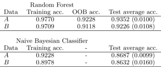
Table 1.Classification accuracy using 810 binary indicators. For the test set, we report the average classification accuracy and its standard deviation between parenthesis.
Random Forest
Data Training acc. OOB acc. Test average acc.
A 0.9770 0.9228 0.9352 (0.0100)
B 0.9709 0.9118 0.9226 (0.0108)
Naive Bayesian Classifier
Data Training acc. - Test average acc.
A 0.9228 - 0.8687 (0.0099)
B 0.8978 - 0.8632 (0.0160)
Table 1 reports the global classification accuracy of the Random Forest and Naive Bayes classifier, using all the indicators. As expected, Random Forests suffer neither from the curse of dimensionality nor from strong over fitting (the test set performances are close to the learning set ones). For the Naive Bayes classifier, those performances are significantly lower than the one obtained by the Random Forest. As shown by the confusion matrix on Table 2, the classification errors are not concentrated on one class (even if the errors are
not perfectly balanced). This tends to confirm that the indicators are adequate to the task (this was already obvious from the Random Forest).
Table 2.Data set A: confusion matrix with all indicators for Naive Bayes classifier on the full test set.
0 1 2 3 total 0 2267 162 32 39 2500 1 118 671 36 4 829 2 26 4 708 91 829 3 46 7 76 700 829 4.5. Feature selection
While satisfactory results are obtained, it would be unrealistic to ask to an operator to review 810 binary values to understand why the classifier favours one class rather than the others. Thus a feature selection should be appropriate.
As explained in Section 3.4, the feature selection relies on the mRMR ranking procedure. A forward approach is used to evaluate how many indicators are needed to achieve acceptable predictive performances. Notice that in the forward approach, indicators are added in the order given by mRMR and then are never removed. As mRMR takes into account redundancy between the indicators, this should not be a major issue. Then for each number of indicators, a Random Forest and a Naive Bayes classifier are constructed and evaluated.
1 10 20 30 40 50 60 70 80 90 100 0.6 0.7 0.8 0.9 1 Number of indicators Classification accuracy A : learning set A : out−of−bag estimate B : learning set B : out−of−bag estimate
Figure 2.Data sets A (black) and B (blue) Random
Forest: classification accuracy on learning set (circle) as a function of the number of indicators. A boxplot gives the classification accuracies on the test subsets, summarized by its median (black dot inside a white circle). The estima-tion of those accuracies by the out-of-bag (oob) bootstrap estimate is shown by the crosses.
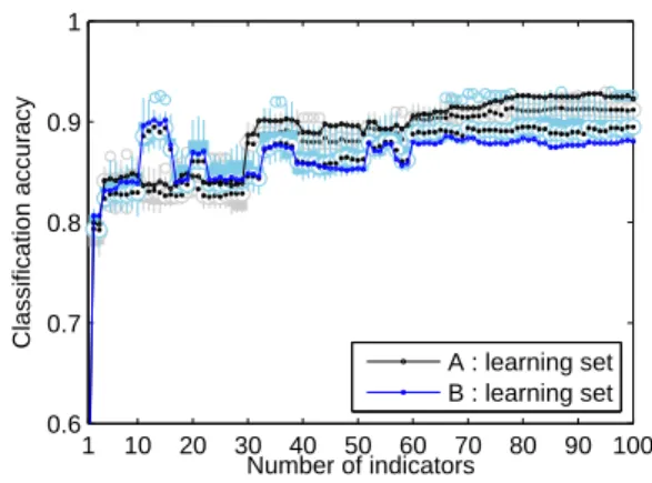
Anomaly Detection 1 10 20 30 40 50 60 70 80 90 100 0.6 0.7 0.8 0.9 1 Number of indicators Classification accuracy A : learning set B : learning set
Figure 3.Data sets A (black) and B (blue) Naive
Bayes classifier: classification accuracy on learning set (circle) as a function of the number of indicators. A box-plot gives the classification accuracies on the test subsets, summarized by its median (black dot inside a white circle).
indicators for sets A and B. The classification accuracy of the Random Forest increases almost monotonously with the number of indicators, but after roughly 25 to 30 indicators (depending on the data set), performances on the test set tend to stagnate . In practice, this means that the proposed procedure can be used to select the relevant indicators implementing this way an automatic tuning procedure for the parameters of the expertly designed scores.
Results for the Naive Bayes classifier are slightly more complex in the case of the second data set, but they confirm that indicator selection is possible. Notice that the learning set performances of the Naive Bayes clas-sifier are almost identical to its test set performances (which exhibit almost no variability over the slices of the full test set). This is natural because the classifier is based on the estimation of the probability of observing a 1 value independently for each indicator, condition-ally on the class. The learning set contains at least 250 observations for each class, leading to a very accu-rate estimation of those probabilities and thus to very stable decisions. In practice one can therefore select the optimal number of indicators using the learning set performances, without the need of a cross-validation procedure.
It should be noted that significant jumps in perfor-mances can be observed in all cases. This might be an indication that the ordering provided by the mRMR procedure is not optimal. A possible solution to reach better indicator subsets would be to use a wrapper ap-proach, leveraging the computational efficiency of both Random Forest and Naive Bayes construction.
Mean-1 10 20 30 40 50 60 70 80 90 100 0 0.2 0.4 0.6 0.8 1 Number of indicators Classification error without anomaly variance shift mean shift trend modification
Figure 4.Data set A Naive Bayes classifier: classifica-tion error for each class on the training set (solid lines) and on the test set (dotted lines, average accuracies only).
while Figure 4 shows in more detail this phenomenon by displaying the classification error class by class, as a function of the number of indicators, in the case of data set A. The figure shows the difficulty of discern-ing between mean shift and trend shift (for the latter, no specific test has been included, on purpose). But as the strong decrease in classification error when the 30-th indicator is added concerns both classes (mean shift and trend shift), the ordering provided by mRMR could be questioned.
4.6. Indicator selection
Based on results shown on Figure 3, one can select an optimal number of binary indicators, while enforcing a reasonable limit on this number to avoid flooding the human operator with too many results. For instance Table 3 gives the classification accuracy of the Naive Bayes classifier using the optimal number of binary indicators between 1 and 20.
Table 3.Classification accuracy of the Naive Bayesian net-work using the optimal number binary indicators between 1 and 20. For the test set, we report the average classification accuracy and its standard deviation between parenthesis.
Data Training acc. Test avg acc. # indicators
A 0.8487 0.8448 (0.0134) 9
B 0.9018 0.8935 (0.0130) 13
While the performances are not as good as the ones of the Random Forest, they are acceptable : the se-lected indicators can be shown to the human operator together with the estimated probabilities of getting a positive result from each indicator, conditionally on each class, shown on Table 4. For instance here the
first selected indicator, conf u(2, 3), is a confirmation indicator for the U test. It is positive when there are 2 windows out of 3 consecutive ones on which a U test was positive. The Naive Bayes classifier uses the estimated probabilities to reach a decision: here the indicator is very unlikely to be positive if there is no change or if the change is a variance shift. On the contrary, it is very likely to be positive when there is a mean or a trend shift. While the table does not “explain” the decisions made by the Naive Bayes classifier, it gives easily interpretable hints to the human operator.
Table 4.The 9 best indicators according to mRMR for data set A. Confu(k,n) corresponds to a positive Mann-Whitney-Wilcoxon U test on k windows out of n consecutive ones. Conff(k,n) is the same thing for the F-test. Ratef(α) cor-responds to a positive F-test on α × m windows out of m. Lseqf(α) corresponds to a positive F-test on α × m consecutive windows out of m. Lsequ(α) is the same for a U test. Detailed parameters of the indicators have been omitted for brevity.
type of indicator no change variance mean trend
confu(2,3) 0.0103 0.011 0.971 0.939 F test 0.0206 0.83 0.742 0.779 U test 0.02 0.022 0.968 0.941 lseqf(0.3) 0.0053 0.571 0.336 0.023 confu(4,5) 0.0343 0.03 0.986 0.959 confu(3,5) 0.0013 0.001 0.923 0.899 confu(2,3) 0.0673 0.06 0.992 0.967 F test 0.042 0.853 0.793 0.813 KS test 0.0113 0.259 0.961 0.923
4.7. Role of confirmation indicators
In table 4, one can see several confirmation indicators. In this section, we illustrate their impacts on results. We use a new simulated data set C. Its random noise is based on a Student distribution (3 degrees of free-dom) but with a random variance. That is n random variables Y1, . . . , Yn independent and identically
dis-tributed according to T (3). X1, . . . , Xn are such that
Xi ∼ aYi where a is chosen uniformly at random in
[0.5, 3]. The same three types of shift are used. But, the mean shift added is chosen uniformly at random in [0.3, 5] and the variance shift is added chosen at random in [1.05, 5].
For C, new tests are added : the Student-test with equal variance and unequal variance (test for shift in mean), a slope shift detection and a slope change test. 2565 indicators are then obtained.
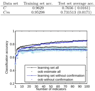
In table 5, the result obtained with and without con-firmation indicators (Cm) is reported. In figure 5, the difference obtained in set C with and without confir-mation indicators is given for the first 100 indicators
according to mRMR. The confirmation indicators im-prove the classification accuracy.
Table 5.Classification accuracy of the Random Forest clas-sifier using all binary indicators : 2565 for set C, 945 for set Cm . Cm is the same data as C but no confirmation indicators are used.
Data set Training set acc. Test set average acc.
C 0.9629 0.7656 ( 0.0161) Cm 0.95298 0.731513 (0.0171) 1 10 20 30 40 50 60 70 80 90 100 0.2 0.4 0.6 0.8 1 Number of indicators Classification accuracy
learning set all oob estimate all
learning set without confirmation oob without confirmation
Figure 5.Data set C (black) and Cm(blue) Random
Forest, see Figure 2 for details. Cm is the same data as C but no confirmation indicators are used.
Acknowledgments
This study is supported by grant from Snecma1
.
5. Conclusion and perspectives
This paper proposes a general methodology that com-bines expert knowledge with feature selection and auto-matic classification to design accurate anomaly detector and classifier. Feature selection allows to reduce the number of useful indicators to a humanly manageable number. This allows a human operator to understand at least partially how a decision is reached by an auto-matic classifier. This is favoured by the choice of the indicators which are based on expert knowledge. A very interesting byproduct of the methodology is that it can work on very different original data as long as expert decision can be modelled by a set of parametric anomaly scores. This was illustrated by working on signals of different lengths.
1Snecma, Safran Group, is one of the worlds leading manufacturers of aircraft and rocket engines, see http: //www.snecma.com/for details.
Anomaly Detection
The methodology has been shown sound using simu-lated data. Using a reference high performance clas-sifier, Random Forests, the indicator generation tech-nique covers sufficiently the parameters space to obtain high classification rate. Then, the feature selection mechanism leads to a reduced number of indicators with good predictive performances when paired with a simpler classifier, the Naive Bayes classifier. As shown in the experiments, the class conditional probabilities of obtaining a positive value for those indicators pro-vide interesting insights on the way the Naive Bayes classifier takes a decision.
In order to justify the cost of collecting a sufficiently large real world labelled data set in our context (engine health monitoring), additional experiments are needed. In particular, multivariate data must be studied in order to simulate the case of a complex system made of numerous sub-systems. This will naturally lead to more complex anomaly models. We also observed possible limitations of the feature selection strategy used here as the performances displayed abrupt changes during the forward procedure. More computationally demanding solutions, namely wrapper ones, will be studied to confirm this point.
It is also important to notice that the classification accuracy is not the best way of evaluating the perfor-mances of a classifier in the health monitoring context. Firstly, health monitoring involves intrinsically a strong class imbalance (Japkowicz & Stephen, 2002). Secondly, health monitoring is a cost sensitive area because of the strong impact on airline profit of an unscheduled maintenance. It is therefore important to take into ac-count specific asymmetric misclassification cost to get a proper performance evaluation. For example, results have shown the role played by confirmation indicators, they are designed to limit false alarm rate.
References
Basseville, M., & Nikiforov, I. V. (1995). Detection of abrupt changes: theory and applications. Journal of the Royal Statistical Society-Series A Statistics in Society, 158, 185.
Breiman, L. (2001). Random forests. Machine learning, 45, 5–32.
Breiman, L., Friedman, J. H., Olshen, R. A., & Stone, C. J. (1984). Classification and regression trees. wadsworth & brooks. Monterey, CA.
Chandola, V., Banerjee, A., & Kumar, V. (2009). Anomaly detection: A survey. ACM Computing Surveys (CSUR), 41, 15.
Cˆome, E., Cottrell, M., Verleysen, M., & Lacaille, J. (2010). Aircraft engine health monitoring using self-organizing maps. In Advances in data mining. appli-cations and theoretical aspects, 405–417. Springer. Flandrois, X., Lacaille, J., Masse, J.-R., & Ausloos,
A. (2009). Expertise transfer and automatic failure classification for the engine start capability system. AIAA Infotech, Seattle, WA.
Fleuret, F. (2004). Fast binary feature selection with conditional mutual information. Journal of Machine Learning Research (JMLR), 5, 1531–1555.
Guyon, I., & Elisseeff, A. (2003). An introduction to variable and feature selection. The Journal of Machine Learning Research, 3, 1157–1182.
Hegedus, J., Miche, Y., Ilin, A., & Lendasse, A. (2011). Methodology for behavioral-based malware analy-sis and detection using random projections and k-nearest neighbors classifiers. Computational Intelli-gence and Security (CIS), 2011 Seventh International Conference on (pp. 1016–1023).
Japkowicz, N., & Stephen, S. (2002). The class imbal-ance problem: A systematic study. Intelligent data analysis, 6, 429–449.
Koller, D., & Friedman, N. (2009). Probabilistic graph-ical models: principles and techniques. The MIT Press.
Kotsiantis, S. B., Zaharakis, I., & Pintelas, P. (2007). Supervised machine learning: A review of classifica-tion techniques.
Lacaille, J. (2009). A maturation environment to develop and manage health monitoring algorithms. PHM, San Diego, CA.
Peng, H., Long, F., & Ding, C. (2005). Feature selec-tion based on mutual informaselec-tion criteria of max-dependency, max-relevance, and min-redundancy. Pattern Analysis and Machine Intelligence, IEEE Transactions on, 27, 1226–1238.
Rabenoro, T., & Lacaille, J. (2013). Instants ex-traction for aircraft engine monitoring. AIAA In-fotech@Aerospace.