HAL Id: hal-01392863
https://hal.inria.fr/hal-01392863
Submitted on 4 Nov 2016
HAL is a multi-disciplinary open access
archive for the deposit and dissemination of
sci-entific research documents, whether they are
pub-lished or not. The documents may come from
teaching and research institutions in France or
abroad, or from public or private research centers.
L’archive ouverte pluridisciplinaire HAL, est
destinée au dépôt et à la diffusion de documents
scientifiques de niveau recherche, publiés ou non,
émanant des établissements d’enseignement et de
recherche français ou étrangers, des laboratoires
publics ou privés.
A New WSN Deployment Approach for Air Pollution
Monitoring
Ahmed Boubrima, Walid Bechkit, Hervé Rivano
To cite this version:
Ahmed Boubrima, Walid Bechkit, Hervé Rivano. A New WSN Deployment Approach for Air Pollution
Monitoring. CCNC 2017 - 14th IEEE Consumer Communications & Networking Conference, Jan 2017,
Las Vegas, United States. �hal-01392863�
A New WSN Deployment Approach for Air
Pollution Monitoring
Ahmed Boubrima
∗, Walid Bechkit
∗and Hervé Rivano
∗∗Université de Lyon, INRIA, INSA-Lyon, CITI-INRIA, F-69621, Villeurbanne, France
Abstract—Due to the increasing industrialization and the massive urbanization, air pollution monitoring is being considered as one of the major challenges of smart cities. Many air pollution monitoring systems have been proposed in the literature, among which wireless sensor networks seem to be a leading solution thanks to sensors’ low cost and autonomy as well as their fine-grained deployment. A careful deployment of sensors is therefore necessary to get better performances while ensuring a minimal financial cost. In this paper, we consider citywide wireless sensor networks and tackle the minimum-cost node positioning issue for air pollution monitoring. We propose an efficient approach that aims to find optimal sensors and sinks locations while ensuring air pollution coverage and network connectivity. Unlike most of the existing methods, which rely on simple and generic detection models, our approach is based on the spatial analysis of pollution data, allowing to take into account the nature of the pollution phenomenon. As proof of concept, we apply our approach on real world data, namely the Paris pollution data, which was recorded in March 2014. We also perform extensive simulations in order to study the performance of our approach in comparison to the existing methods.
Keywords— Smart city, Air pollution monitoring, Detec-tion of threshold crossings of pollutants, Spatial data cluster-ing, Wireless sensor networks (WSN), Deployment, Coverage, Connectivity.
I. INTRODUCTION
Air pollution is traditionally monitored with conventional measuring stations equipped with multiple sensors. These systems are usually inflexible and expensive. An alternative solution would be to use wireless sensor networks (WSN), which consist of a set of nodes that can measure different pollutant concentrations and send them to some base stations through particular nodes called sinks [1]. The use of WSN for air pollution monitoring may have a great interest, which can be mainly ascribed to the autonomy and cost reduction of nodes in addition to their fine spatial and temporal granularity. When using wireless sensor networks for air pollution mon-itoring, one the following objectives may be targeted: i) the periodic air quality sampling and ii) the detection of threshold crossings in order to trigger adequate alerts. In this work, we focus on the second application and tackle the minimum-cost deployment issue of pollution sensors.
Minimizing the deployment cost is a major challenge in WSN design. The problem consists in determining the optimal positions of sensors and sinks so as to cover the environment and ensure the network connectivity while minimizing the deployment cost [2]. This latter may include the financial cost of nodes, the energy cost, etc. Coverage issue commonly known as k-coverage problem, requires that at least k sensors monitor each interest point. The network is said connected if
each sensor can communicate information to at least one sink [2]. For simplicity’s sake, most papers on WSN deployment assume that two nodes are able to directly communicate with each other if the distance between them is less than a radius called the communication range [3]. Most research work on coverage use a simple detection model which assumes that a sensor is able to cover a point in the environment if the distance between them is less than a radius called the detection range [4]. This can be true for some applications like presence sensors but is not suitable for pollution monitoring. Indeed, a pollution sensor can only detect pollutants that come into contact with it, and thus such a sensor does not have a detection zone like presence sensors.
Unlike the deployment methods that are based on generic detection models, we propose an efficient 4-step approach based on spatial analysis of air pollution data. In the first step, we identify the air pollution zones where sensors have to be deployed using ZSCAN, an extension of DBSCAN which is a well-known and widely used spatial data clustering algorithm [5]. The obtained zones will be then grouped in a set of sites based on their intersections. In the third step, we propose a new integer linear programming formulation (ILP) that allows to perform a minimum-cost deployment of sensors in each site while ensuring pollution coverage and network connectivity in a joint way. Finally, a sink is placed in each site so as the obtained WSN is multi-sink.
The contributions of our work can be summarized in the following points: i) we propose a new deployment approach based on air pollution data analysis and adequate ILP models; ii) we propose in the first step of our approach an extension of the DBSCAN clustering algorithm in order to identify air pollution zones; iii) we propose in the third step a new coverage and connectivity ILP formulation based only on flows; and finally iv) we apply our approach on real pollution data of Paris and study its performance in comparison to the state-of-the-art methods.
The remainder of this paper is organized as follows. We review the main research work on integer programming formulations of WSN deployment in section II and the spatial data clustering algorithms in section III. Section IV details our approach and explains the 4 processing steps while section V shows the simulation data set and the obtained results. Finally, we conclude and present some perspectives in section VI.
II. RELATEDWORK
Several integer linear programming formulations have been proposed in the literature to formulate WSN coverage and connectivity issues [6]. Chakrabarty et al. [4] tackled the
coverage issue while representing the environment as a two or three dimensional grid of points which form the sensor field to be covered, and proposed first a nonlinear model for minimizing the cost of sensors deployment while ensuring complete coverage of the sensor field. Then, they applied some transformations to linearize the first model and obtain an ILP formulation. The authors assume that the points to be covered are the same on which sensors should be placed, and formulate coverage based on the distance between the different points of the environment. Therefore, each sensor has a circular detection area which defines the points that it can cover.
Chakrabarty et al.’s model suffers from the intractability since it is based on a nonlinear formulation. In addition, sensors may have a non-circular detection area. Meguerdichian and Potkonjak [7] deal with all these drawbacks and propose an ILP formulation of coverage based on the Set Covering Problem, which is a well-known combinatorial problem. They consider a set of positions where sensors can be placed and a set of discrete points approximating the sensor field. A sensor can have a detection area with a shape which is not necessarily circular. This ILP model does not take into account sensors with different costs and consider only the 1-Coverage where a point should be covered by only one sensor.
The models proposed in [4] and [7] do not take into account the different coverage requirements of the environment points, instead the authors assume uniform coverage where all the points in the sensor field have to be covered by the same number of sensors. This may be unrealistic in some applications where some zones in the environment are more critical than others. Altinel et al [6] focused on this issue and proposed an integer linear programming formulation that considers different coverage requirements among the sensor field points. They also show that their model can deal with connectivity under the assumption that the transmission range is as least equal the double of the detection range. This cannot be true in most of the applications since sensing and transmission are two independent functionalities of sensors.
Connectivity constraint has been studied in different con-texts including topology control and deployment issues. Most of the existing models are based on the flow concept [3], [8], [9]. These formulations assume that each sensor generates a flow unit and check whether the generated units can be recovered by sink nodes. In some models [3], sinks were considered already located and deployment modeling treats only sensor nodes. The other models [8], [9] consider the two types of nodes, sensors and sinks. However, all these models assume that the potential positions of sinks are different from those of sensors. This cannot be applied in some applications where a potential position can correspond to both sensors and sinks.
In some other works, authors suppose that a set of con-nected sensors that ensure coverage are already deployed, and propose integer programming formulations to find optimal sinks locations and sensors-to-sinks routes. Authors in [10] evaluate firstly the shortest path cost between each sensor and potential sink location using the Dijkstra algorithm. Two main metrics were proposed to compute shortest paths: energy cost and financial cost. In the second case, the proposed ILP model aims to find the optimal sinks positions while minimizing the financial cost of the sinks deployment and the sensors-to-sinks
routing. Two other formulations based on flows were proposed in [11] where authors present a single commodity flow and a multi-commodity flow formulations. However, they show that the integer programming model presented in [10] is better. Moreover, they propose and test good heuristics for this latter. Unfortunately, all the works presented in this section suppose that a sensor is able to cover points within its detection range. This cannot be directly applied to air pollution monitoring since a pollution sensor can only detect pollutants that come into contact with it. Moreover, the coverage and con-nectivity constraints are modeled independently in the sense that coverage is formulated by analogy to the Set Covering Problem and connectivity formulation is based on the flow concept. In section IV, we address these issues while proposing an ILP formulation based on air pollution data clustering, and treat the joint modeling of coverage and connectivity using only the flow concept.
III. SPATIAL DATA CLUSTERING
Spatial data clustering is the process of grouping objects based on their spatial locations similarity in addition to other features like temperature and pollution concentration values [5]. The most common methods used to cluster spatial data are density based algorithms [5]. The principle of these methods is to group data having closer density and identify the rest as noise data. The density of a cluster is defined as the average number of neighbors of the cluster objects. Density-based clustering methods perform well on spatial databases and can generate clusters with different shapes and sizes.
DBSCAN (A Density-Based Algorithm for Discovering Clusters in Large Spatial Databases with Noise) was the first to introduce the density-based clustering principle. Based on this concept, it aims to identify clusters with similar densities in large spatial databases [12]. Three types of data objects are defined before to process the algorithm: core data, border data and noise data. Core data correspond to objects that are inside clusters, points that are at the border of a cluster are called border points and the rest is called noise points. DBSCAN starts by identifying core points. The neighborhood of these points is then expanded to form clusters. This principle allows finding clusters with different shapes and sizes.
Several extensions have been proposed for DBSCAN, among which VDBSCAN (Varied Density Based Spatial Clus-tering of Applications with Noise), which is aims to find meaningful clusters that have different densities [13]. The idea behind VDBSCAN is to adapt DBSCAN parameters to database structure, which leads to better clustering results. An-other extension of DBSCAN is ST DBSCAN (Spatial-temporal DBSCAN) which can deal with temporal data attributes in addition to spatial attributes [14]. Furthermore, ST-DBSCAN is able to solve conflicts in border objects and assigns well these points to the most meaningful cluster.
DBSCAN and its variants can be used in several ap-plications thanks to their density-based structure. However, these algorithms don’t take into account the dispersion of pollution particles and gases. In the next section, we show how DBSCAN exploration principle can be adapted to locate high-pollution-concentration areas in a given city.
IV. PROPOSAL
A. Main inputs
In order to deploy sensors efficiently in the city, our approach requires as a primary input, air pollution spatial data. Given a pollutant to monitor, this consists on estimated values of the pollutant concentrations in the whole city for different time instants. These concentrations can be estimated using atmospheric pollution dispersion models based on pollutants sources locations and meteorological data. They can also be obtained using interpolation algorithms based on some measurements established by a set of monitoring stations or by combining the two first methods. In the following, we denote by T the set of time instants when pollution is estimated, and I the set of spatial points representing the city. The second set is defined by applying a high resolution discretization process. For each time instant t ∈ T and spatial point i ∈ I, let Ct,i
denote the estimated or measured pollution concentration. In addition to air pollution estimated concentrations, the approach requires also data on sensors potential positions, this corre-sponds to positions where sensors can be deployed. On one hand, in smart cities applications, some restrictions on node positions may apply because of public regulations or practical issues, e.g. the availability of a pole on which a sensor can be secured. On the other hand, in order to alleviate the energy constraints, we may place sensors on lampposts and traffic lights. We denote in what follows the set of positions where sensors can be deployed by P.
B. Workflow
The deployment operation is performed through four steps based on the air pollution data and the sensors potential positions. First, a spatial clustering algorithm is applied to the air pollution data in order to determine pollution zones that are due to the same pollutant sources. To this end, we propose an exploratory algorithm, based on DBSCAN, that starts by identifying points where pollution concentration peaks occur. Then, the neighborhood of each pollution peak is explored to construct the corresponding pollution zone. We denote by Z the set of these zones. In the second step, the pollution zones will be grouped in order to define a set of deployment sites, denoted by S. Each site s ∈ S corresponds to a region in the city, and consists of a subset of pollution zones Zs ⊂ Z. We denote the subset of sensors potential
positions that belong to each site s ∈ S by Ps ⊂ P. In
the last two steps, a mono-sink wireless sensor sub-network will be deployed in each site s ∈ S so as to cover all the pollution zones z ∈ Zswhile minimizing the deployment cost.
As a result, the global wireless sensor network is multi-sink. We propose in the third step an integer programming model which determines a connected sensors sub-network, defined by the optimal positions Bs ⊂ Ps, that ensures pollution
monitoring in the site s. Pollution monitoring is ensured by deploying at least one sensor in each pollution zone to ensure the coverage constraint. Finally, in the fourth step, another ILP is proposed in order to locate sink on one of the selected positions p ∈ Bs so as that an objective function is optimized
(energy consumption, end-to-end transmission delay, etc.). In this paper we investigate the use of urban facilities in order to alleviate the energy constraints, and therefore, consider the minimization of the sensor-to-sink maximum delay without
loss of generality. The notations used in our approach are summarized in table I.
Notation Description
T Set of time instants of pollution estimations I Set of discrete points of pollution estimations P Set of potential positions of sensors and sinks Z Set of pollution zones
S Set of deployment sites Zs Set of pollution zones within the site s
Ps Set of sensors potential positions within the site s
Bs Set of sensors selected positions within the site s
TABLE I: Summary of the approach notations. C. Step 1: pollution zones identification
The first step of our approach aims to identify pollution zones where sensors will be deployed. For this purpose, we propose ZSCAN, an extension of DBSCAN. This algorithm will be applied to the estimated concentrations in order to cluster points that belong to the same pollution zone. Algorithm 1 ZSCAN
Inputs: T , I, {Ct,i; t ∈ T , i ∈ I}
Output: Z Z ← ∅ for t ∈ T do
Mark all the points in I as unvisited repeat
Let i be the unvisited point having the highest concentration Ct,i
z ← construct(i, t)
Mark all the points in z as visited z ← f ilter(z, ∆C)
z ← points_to_polygon(z) Z ← Z ∪ {z}
until all the points in I are visited
As presented in Algorithm 1, ZSCAN identifies all the pollution zones occurring in each time instant. To this end, pollution peaks, points having the highest pollution concen-tration, are first identified. A pollution zone is created every time a peak is identified using the construct function, which starts by adding all the neighbors of the pollution peak i to the zone under construction. The neighborhood of a point in the map is defined as the set of closer and unvisited points whose pollution concentration estimated in t is less. The neighbors of each chosen point are then added to the current zone. This process stops when it arrives at a point whose neighborhood set is empty, meaning that its neighbors have higher pollution concentration values. Once the current pollution zone is completely identified, a filtering function is applied to keep only points where pollution concentration is sufficiently closer the peak value, i.e. points where pollution concentration difference with the peak value is less than a threshold that we denote by ∆C. This increases the chance that a sensor deployed in the detected zone is able to monitor the corresponding pollution sources. At the end, a geometrical form is given to the found zone by applying the function points_to_polygon. The main difference between DBSCAN and ZSCAN is that this latter visits points in an ordered way, starting by pollution peaks, and then expands the peak neighborhood to detect pollution zones.
D. Step 2: deployment sites determination
In this step, a set of deployment sites is determined. Each site corresponds to a subset of pollution zones Z that are connected. Algorithm 2 presents the proposed method for this purpose. First, an undirected graph G is defined such that each pollution zone represents a vertex and each intersection in the set Z corresponds to an edge in this graph. Next, the set of connected components of the graph G that we denote by C is computed. A deployment site is then defined as the region of the city that is formed by a connected component.
Algorithm 2 SITES-IDENT Input: Z
Output: S S ← ∅
Let G = (V, E ) be an undirected graph V ← Z E ← {(z1, z2) ∈ Z × Z where z1∩ z26= ∅} C ← Connected_Components(G) for c ∈ C do s ← ∪z∈c{z} S ← S ∪ {s}
E. Step 3: sensors deployment
In this step, we deploy a mono-sink sensor sub-network in each site s ∈ S. We first define a flow oriented graph G = {V, A} where vertices set V corresponds to the pollution zones and the sensors potential positions of the site s, i.e. Zs∪ Ps.
We notice that each zone is considered as a single vertex. Let A(i) denote the neighborhood of i ∈ V . We define a first set of arcs from each pollution zone z ∈ Zs to sensor potential
positions p that are within its region, i.e. p ∈ z. A second set of arcs is defined from each sensor potential position p ∈ Psto
positions which are in its communication range that we denote by Γ(p).
The idea of our modeling is that each pollution zone inserts one flow unit in the network through the first set of arcs. For a given selected positions of sensor nodes, the latter ensures network coverage and connectivity if and only if the received units from pollution zones can be forwarded by these nodes through the second set of arcs so that a chosen pollution zone can recover all the generated units (which ensures the connectivity of the defined graph). This particular zone does not generate units but recovers all of them from a sensor that is placed within its region. With these considerations, the selected sensor positions ensure jointly coverage and connectivity if the recovering pollution zone gets all the flow units generated by the other pollution zones and forwarded by the selected sensors. Indeed, Flow passing in the first set of arcs guaranties coverage, and connectivity is verified due to flow forwarded by only selected positions through the second set of arcs. In what follows, we choose the first pollution zone Zs0 to be the one
that recovers flow units, meaning that the other zones generate, each one, a unique flow unit.
We use binary decision variables xp to specify if a sensor
should be placed at a position p or not. Sensors cost may depend on their positions, thus we denote by costp the cost
of deploying a sensor at a position p. We also define the
positive integer decision variables fij as the flow quantity
transmitted from i to j. The flow domain is set to {0, |Zs|−1}
when j = Z0
s in order to ensure that Zs0 recovers the units
from only one sensor. The proposed model ILP 1 minimizes the overall deployment cost as formulated in the objective function. Constraints 2 ensure that each pollution zone except the first one generates exactly a flow unit. Sensors are flow conservative thanks to constraints 4. Constraints 5 ensure that sensors that are not selected (xp = 0) do not participate in
communication. This means that generated flow units will be transmitted by only present sensors. Finally, the first pollution zone receives all the generated units, thanks to constraint 3.
[ILP 1] M inX p∈Ps costp∗ xp (1) S.T. X p∈z fzp = 1, z ∈ Zs− {Zs0} (2) X p∈Z0 s fpZ0 s = |Zs| − 1 (3) X q∈A(p) fpq− X q∈A(p) fqp= 0, p ∈ Ps (4) X q∈A(p) fpq<= (|Zs| − 1) ∗ xp, p ∈ Ps (5)
F. Step 4: sinks location
The last step of our approach consists in locating the sink on one of the sensors selected positions, Bs, so as an
objective function is optimized (energy consumption, end-to-end transmission delay, etc.). As we are investigating the use of urban facilities in this work, i.e. energy constraints are alleviated, we will consider the sensor-to-sink delay. We first determine shortest paths between all the pairs of the set Bs using the delay metric. Let mpl denote the delay value
assigned to the path from p to l. We use binary decision variable yl, l ∈ Bs to specify whether l is the chosen sink
position or not, thus only one yl can be set to one. The
ILP 2 optimization model is based on the works presented in [10], [11] and aims to find an optimal sink location that minimizes the maximum delay in the network, denoted m∗, as formulated in the objective function. The resulting network is mono-sink thanks to constraint 7. Constraints 8 ensure that m∗ corresponds to the highest sensor-to-sink path value with respect to the optimal sink position, i.e. l where yl= 1.
[ILP 2] M in m∗ (6) S.T. X l∈Bs yl= 1 (7) m∗≥ mpl∗ yl, p, l ∈ Bs (8)
V. SIMULATION RESULTS
A. Dataset
We evaluate our approach on a pollution dataset of the Paris city while we focus on monitoring N O2 pollutant particles
(Nitrogen dioxide). The pollution dataset was provided by Air-Parif, a French air quality monitoring association. We based on pollution data measured by 22 monitoring stations to estimate pollutant concentrations in the whole city. Because pollution achieved maximum values in Paris in March 2014 [15], we decided to base on pollution estimation for some periods of this month where pollution concentrations were high. Overall, we constructed 10 snapshots of pollution concentrations. We used the kriging interpolation method to estimate the pollution values with a map resolution of 100 meters. A set of 21201 spatial data records was then obtained for each snapshot. In addition to pollution data, we used lamppost locations as sen-sors potential positions P. The lampposts dataset was provided by the open data service of the Paris city. We summarize in table II the common values of simulation parameters.
Parameter value
Map discretization resolution (for set I) 100m Number of time instants (set T ) 10 ∆C (used in ZSCAN) 5µg/m3
Sensors communication range (used for Γ(p), p ∈ P) 100m Sensors cost (costp, p ∈ P) 1 unity (constant)
TABLE II: Summary of common simulation parameters B. Proof of concept
The first step of the deployment approach is the execution of ZSCAN to identify pollution zones where sensors will be deployed. Pollution peaks are first detected and then expanded to form these zones. Points in each obtained pollution zone have as maximum concentration difference with the pollution peak of the zone 5µg/m3, this corresponds to the value of the
parameter ∆C as mentioned in table II. A number of pollution zones is extracted from each time snapshot. The execution of the spatial clustering algorithm identified 29 pollution zones that occurred in March 2014, these zones are depicted in Figure 1. We notice that some zones occur in different snapshots with a little bit different shape. This is because these zones correspond usually to the same pollutant sources, the different shapes are due to the evolution of weather conditions.
The second step is to group pollution zones that share intersections into a region site where a mono sink sensor network will be deployed. In this simulation case, four sites were identified and are illustrated in Figure 1.
In the third step, we execute the ILP 1 optimization model to find sensors optimal positions based on the generated pollution zones. The ILP model is executed on each site to locate sensors ensuring coverage and connectivity. The results are depicted in Figure 1. The latter shows that sensors are placed in intersections in order to minimize the financial cost. In addition to sensors placed to ensure pollution zones coverage, Figure 1 shows that some sensors are deployed in order to ensure the network connectivity.
Finally, in the last step, we execute the sink location optimization model, ILP 2, that identifies the optimal positions of sinks while minimizing the maximum sensors-to-sink delay. We consider in our tests that the delay is linearly proportional
to the hop count to the sink. Results are depicted in the same figure 1. We notice that sinks are placed in the center of each sub-network, which minimizes the maximum hop count and thus the maximum sensor-to-sink communication delay.
Fig. 1: Proof-of-concept C. Comparison results
In this section, we compare our approach to the litera-ture generic formulation (i.e. coverage and connectivity are modeled independently, coverage is formulated by analogy to the Set Covering Problem using a basic detection model and connectivity formulation is based on the flow concept).
1) Coverage: The coverage formulation given in our ap-proach takes into account the nature of the phenomenon based on spatial analysis of pollution data. This is not the case of the generic formulation given in the literature, which assumes that a sensor is able to detect pollutants within a detection range, i.e. pollution is homogeneous within the detection range of a sensor. Even though this assumption is unrealistic since sensors can only detect pollutants that come into their contact, we compare in this simulation scenario the coverage cost given by our approach and the generic formulation. We depict in Fig. 2 the coverage deployment cost of sites 2 and 3 obtained using the generic formulation while considering different values of detection range compared to our method. Fig. 2 shows that our approach is at least 5 times better than the generic approach when the detection range is less than or equal to 500m. The coverage cost computed by the generic approach decreases when the detection range increases. However, our approach remains better since pollution cannot be homogeneous, as assumed in the generic approach, especially within very large detection ranges.
Fig. 2: Optimal coverage deployment cost given by the generic formulation depending on the detection range of sensors.
2) Execution time: In this simulation scenario, we evaluate the execution time of our approach and establish a comparison with the generic formulation of the literature where cover-age and connectivity are modeled independently. We depict in table III CPU times of the two deployment approaches corresponding to site 2 while considering different values of communication range. Table III shows that our approach is at least around two times faster than the generic approach of the literature. In some cases, when the communication range is equal to 50m for instance, our approach is executed in few minutes while the generic approach takes around an hour to be executed, thanks to the joint formulation of coverage and connectivity principle of our approach. We also notice in table III that the larger the communication range, the lesser the execution time. This can be explained by the fact that less nodes will be used to ensure connectivity in this case.
Communication range Our approach Generic approach 50 m 225 s 3224 s 60 m 807 s 1706 s
70 m 197 s 887 s
80 m 96 s 168 s
TABLE III: Execution time comparison between our approach and the generic approach depending on different values of communication range (the detection range is set to 300m). D. Evaluation of the connectivity cost
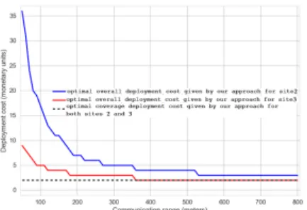
After comparing our approach to the literature generic approach, we now analyze the deployment cost given by our approach for sites 2 and 3 while considering different values of communication range. We plot in Fig. 3 the obtained results. We recall that the optimum value of deployment cost when connectivity constraint is not taken into account is equal to 2 as shown in Fig. 3. We notice that the larger the communication range, the smaller the deployment cost is. This is expected since using a larger communication range allows to minimize the number of nodes used to connect sensors which are positioned within pollution zones. Fig. 3 also shows that when the communication range increases significantly, the overall deployment cost tends to the coverage deployment cost.
Fig. 3: Optimal deployment cost given by our approach de-pending on the communication range of nodes.
VI. CONCLUSION AND FUTURE WORK
In this paper, we propose a new deployment approach that relies on pollution data analysis in order to determine optimal positions of sensors and sinks while minimizing the deployment cost and ensuring air pollution monitoring. Our approach runs on air pollution concentrations and processes
the input data over four steps: pollution zones identification, deployment sites determination, sensor positioning and sinks location. The obtained results showed how our proposal is able to guideline optimal choices for WSN deployment for air pollution monitoring. More generally, the proposed approach can be of a major interest to associations of air pollution monitoring and local authorities. In our future work, we aim at extending the different components of our approach, mainly the ZSCAN algorithm and the joint coverage-connectivity ILP model. Moreover, we will perform simulations on pollution dataset with a longer time period as well as considering other urban cities. A
CKNOWLEDGMENT
This work has been supported by the "LABEX IMU" (ANR-10-LABX-0088) and the "Programme Avenir Lyon Saint-Etienne" of Université de Lyon, within the program "Investissements d’Avenir" (ANR-11-IDEX-0007) operated by the French National Research Agency (ANR).
REFERENCES
[1] J. Yick, B. Mukherjee, and D. Ghosal, “Wireless sensor network survey,” Computer networks, vol. 52, no. 12, pp. 2292–2330, 2008. [2] M. Younis and K. Akkaya, “Strategies and techniques for node
place-ment in wireless sensor networks: A survey,” Ad Hoc Networks, vol. 6, no. 4, pp. 621–655, 2008.
[3] M. Cardei, M. O. Pervaiz, and I. Cardei, “Energy-efficient range assignment in heterogeneous wireless sensor networks,” in ICWMC’06. International Conference on. IEEE, 2006, pp. 11–11.
[4] K. Chakrabarty, S. S. Iyengar, H. Qi, and E. Cho, “Grid coverage for surveillance and target location in distributed sensor networks,” Computers, IEEE Transactions on, vol. 51, no. 12, pp. 1448–1453, 2002.
[5] S. Shekhar, J. Kang, and V. Gandhi, “Spatial data mining,” in Encyclo-pedia of Database Systems, L. LIU and M. ÖZSU, Eds. Springer US, 2009, pp. 2695–2698.
[6] ˙I. K. Altınel, N. Aras, E. Güney, and C. Ersoy, “Binary integer programming formulation and heuristics for differentiated coverage in heterogeneous sensor networks,” Computer Networks, vol. 52, no. 12, pp. 2419–2431, 2008.
[7] S. Meguerdichian and M. Potkonjak, “Low power 0/1 coverage and scheduling techniques in sensor networks,” Citeseer, Tech. Rep., 2003. [8] M. E. Keskin, ˙I. K. Altınel, N. Aras, and C. Ersoy, “Wireless sensor network lifetime maximization by optimal sensor deployment, activity scheduling, data routing and sink mobility,” Ad Hoc Networks, vol. 17, pp. 18–36, 2014.
[9] M. Patel, R. Chandrasekaran, and S. Venkatesan, “Energy efficient sensor, relay and base station placements for coverage, connectivity and routing,” in IPCCC 2005. 24th IEEE International. IEEE, 2005, pp. 581–586.
[10] E. Guney, I. Altinel, N. Aras, and C. Ersoy, “Efficient integer pro-gramming formulations for optimum sink location and routing in wireless sensor networks,” in ISCIS’08. 23rd International Symposium on. IEEE, 2008, pp. 1–6.
[11] E. Güney, N. Aras, ˙I. K. Altınel, and C. Ersoy, “Efficient integer programming formulations for optimum sink location and routing in heterogeneous wireless sensor networks,” Computer Networks, vol. 54, no. 11, pp. 1805–1822, 2010.
[12] M. Ester, H.-P. Kriegel, J. Sander, and X. Xu, “A density-based algorithm for discovering clusters in large spatial databases with noise.” in Kdd, vol. 96, no. 34, 1996, pp. 226–231.
[13] P. Liu, D. Zhou, and N. Wu, “Vdbscan: Varied density based spatial clustering of applications with noise,” in Service Systems and Service Management, 2007 International Conference on, June 2007, pp. 1–4. [14] D. Birant and A. Kut, “St-dbscan: An algorithm for clustering
spatial-temporal data,” Data & Knowledge Engineering, vol. 60, no. 1, pp. 208–221, 2007, intelligent Data Mining.
[15] A. A. L. Kama, H. Hammadou, B. Meurisse, and C. Papaix, “Le pic de pollution a paris du 12 au 17 mars 2014,” Tech. Rep.