Characterization of low-frequency electric potential oscillations near the edge of a plasma confined by a levitated magnetic dipole

Characterization of low-frequency electric

potential oscillations near the edge of a plasma

confined by a levitated magnetic dipole.

by

Ryan M. Bergmann

Submitted to the Department of Nuclear Science and Engineering

in partial fulfillment of the requirements for the degrees of

Bachelor of Science in Nuclear Science and Engineering MASSACHUSETTS _NSTMU

and

Master of Science in Nuclear Science and Engineering

_AUG

_{19 2009}

at the

MASSACHUSETTS INSTITUTE OF TECHNOLOGY

_LIBIRARIES

June 2009

©

Massachusetts Institute of Technology 2009. All rights reserved.

ARCHIVES

Author....

'1

Depar

gd of Nuclear Science and Engineering

May 8, 2009

Certified by

Jay Kesner, MIT

Senior Scientist

Thesis Supervisor

....

D rren

...

...

Read by

SP

fessor of

Research Scientist

Thesis Supervisor

David G. Cory

Niclear Engineering

Thesis Reader

Accepted

by...

I/ /

_{Jacquelyn C. Yanch}

Chairman, Department Committee on Graduate Theses

y

Characterization of low-frequency electric potential

oscillations near the edge of a plasma confined by a levitated

magnetic dipole.

by

Ryan M. Bergmann

Submitted to the Department of Nuclear Science and Engineering on May 8, 2009, in partial fulfillment of the

requirements for the degrees of

Bachelor of Science in Nuclear Science and Engineering and

Master of Science in Nuclear Science and Engineering

Abstract

A vertically adjustable electrostatic probe array was made to observe the previously seen low-frequency angular oscillations in LDX and identify if they are related to computationally expected convective cells. The array rests one meter from the centerline and measures edge fluctuations at field lines near the separatrix. It spans ninety degrees and has 24 probes mounted on it for total probe tip separation of 6.8cm. Bispectral analysis of the fluctuations show that that an inverse cascade of energy is present at times in LDX. The cascade transfers energy from small spatial scale structures to large scale structures. The wavenumber spectrum is xc k- 1.4 to oc k-25 at high wavenumbers, which encompasses the inverse energy cascade regime of c k- 5

/3. The plasma also has a linear dispersion relation which gives a phase velocity of 2-16 k. This phase velocity is inversely correlated with neutral gas pressure in the vessel. The velocity also has a local maximum at 5 pTorr which is the pressure that produces maximum plasma density. The radial E x B drift velocities are observed to have a mean near zero, which indicates a closed structure like a convective cell. The instantaneous radial drift velocities are on the order of the ion sound speed, which is 35 km/s.

Thesis Supervisor: Jay Kesner, MIT Title: Senior Scientist

Thesis Supervisor: Darren T. Garnier, Columbia University Title: Research Scientist

Acknowledgments

I would like to thank Darren Garnier and Jay Kesner for the great opportunities they have given me during my stay with LDX, the lessons and experience they have shared, and the doors they have opened for me. Rick Lations and Don Strahan for their mechanical insight and assistance that saved me hours of work while constructing the probe array. Brian Grierson for his help with bispectral analysis, since it probably wouldn't be present in this thesis if he hadn't guided me. I would also like to thank my parents for their unwavering encouragement and support not only through my college and graduate years, but through my whole life. I would be nowhere without them. I would also like to thank my siblings Mike, Amy, and Becky for their encouragement, kind words, care packages, and insights. Last be not least, I would like to thank Amanda Baker for her uncanny ability to keep me sane when things looked grim and the happiness she brings into my life.

Contents

1 Introduction

1.1 The Levitated Dipole Experiment . ... 1.2 Energy Cascades ...

1.3 Electrostatic Probe Array ...

2 Theory

2.1 Probes ...

2.1.1 Floating Potential ...

2.1.2 Frequency Response ...

2.2 Inverse Energy Energy Cascades in Plasma Fluctuations ... 2.3 The Ritz Bispectral Method ...

2.4 Phase Velocity, Drifts, and Wavenumber Spectrum ... 3 Experimental Setup

3.1 Probe Array Design

3.1.1 Mechanical 3.1.2 Electrical 3.1.3 Probes . . 31 36 36 44 44 . . . . . . . . . . . . . . . .° . . . . . . . . . . . . . . . . . . . . . . . . . . . . . . . ... . . . . . . . . . . . . . . . .

4 Experimental Observations 55

4.1 ExB Drift ... ... ... 56

4.2 Fluctuation Phase Velocity ... ... 57

4.3 Bispectral Analysis ... ... 62 4.3.1 Shot 81003019. ... ... 63 4.3.2 Shot 81217011 ... . ... 68 4.3.3 Shot 90312025 ... ... 72 4.3.4 Shot 90312028 ... ... 75 4.3.5 Divergent Analysis ... .. . . 78 4.3.6 Time Analysis ... ... 81 4.4 Power Spectra ... ... 83 5 Conclusions 87 A Hardware 93

List of Figures

2-1 Schematic of a Langmuir probe . ... ... .. 8

2-2 I-V curve of typical LDX plasma . ... . . . . 10

2-3 Synthetic signal construction ... . ... 20

2-4 3-wave coupling illustration ... .... 20

2-5 Window sampling in time ... ... 21

2-6 Comb and its transform ... ... 23

2-7 Progression of sampling kernels as more points are added in time. . 24 2-8 Effect of finite sampling in time on frequency spectrum construction. 24 2-9 Black box modification fo signals ... . 25

2-10 Linear transfer function used to produce the synthetic data ... 26

2-11 Quadratic transfer function used to produce the synthetic data . . .. 26

2-12 Computational results from synthetic test data ... 27

3-1 LDX overview ... ... 32

3-2 Probe array position . . . ... ... ... 34 vii

3-3 The probe array position relative to the field lines at the separatrix. The red line shows the direction of the magnetic field at that point. The ExB direction measured by the array is at a right angle to the red line, pointing radially inwards. The blue line shows the field line intersecting the probe tip. ...

3-4 The probe array position relative to the field lines at full insertion. The red line shows the direction of the magnetic field at that point. The ExB direction measured by the array is at a right angle to the red line, pointing radially inwards. The blue line shows the field line intersecting the probe tip.

3-5 The total probe array . . ... 3-6 The probe array installed in LDX ... 3-7 A probe tip. ...

3-8 The PEEK insulator and solid copper conductor. 3-9 Probe array structural detail . ...

3-10 Detail of the probe holder and terminal block highlighting

3-11 3-12 3-13 3-14 3-15 3-16 3-17 3-18

and connection pins/sockets ... Probe array SolidWorks simulation Movement parts diagram . . . . PLC . ...

Probe Electrical layout . . . .. Signal cable ...

Amplifier topology . . . ... Simulation gain curve . . . .. Measured gain curve . ...

.. . . . 36 .. . . . . 37 the resistor .. . . . . . . . 39 .. . . . . . . . . . 40 .. . . . . 41 .. . . . . . 42 .. . . . 44 .. . . . 46 .. . . . . 47 .. . . . 48 ..... . . . . . . . . 4 8 3-19 Probe gains at lkHz viii .. . . . . . . . . . . 34

3-20 3-21 3-22 3-23 3-24 3-25 3-26 4-1 4-2 4-3 4-4 4-5 Amplifier SNR ... Signal and noise tests . ...

The amplifier box showing the amplifier stack, thickness, and electrical gasket. . .

Amplifier bottom . ... Amplifier top ... Jog problem ...

Fixed jog ... ....

Electric Field and ExB drift . . . . Plasma rotational velocity . . . . . Plasma rotational velocity . . . . . Plasma density vs. neutral pressure Dipole Simulation Results . . . . . 4-6 Bispectrum and transfer coef. conve 4-7 Temporal and spatial spectrograms 4-8 4-9 4-10 4-11 4-12 4-13 4-14 4-15 4-16 4-17

internal cabling, wall

. . . . . . . . . 50 ... . . . . 5 1 .... . . . . . . 5 1 . ... . . . 53 ... . . 53 . . . . . . . . . 57 58 . . . . . . . . . . . 59 . . . . . . . . . . 60 . . . . 6 1 rgence in shot 81003019. ... 64 of shot 81003019. . ... 65

Spatial analysis during 11.5 to 12.5 seconds in shot 81003019 Spatial analysis during 14.8 to 15.8 seconds in shot 81003019 Temporal and spatial spectrograms of shot 81217011.

Spatial analysis during 0.5 to 1.5 seconds in shot 81217011 Spatial analysis during 15.5 to 16.5 seconds in shot 81217011 Time and spatial spectrograms of shot 90312025... Spatial analysis during 0.9 to 1.9 seconds in shot 90312025 . Temporal and spatial spectrograms of shot 90312028... Spatial analysis during 1 to 2 seconds in shot 90312028 . Divergent results after one iteration . ...

Divergent results after twenty iterations . . . . Temporal results . . ...

Power fit to large wavenumbers in shot 81003019. Power fit to large wavenumbers in shot 81003019. Power fit to large wavenumbers in shot 81217011. Power fit to large wavenumbers in shot 81217011 . Power fit to large wavenumbers in shot 90312025. Power fit to large wavenumbers in shot 90312028. A-1 Amplifier pcb layout ...

4-18 4-19 4-20 4-21 4-22 4-23 4-24 4-25 . . . . . 80 . . . .. 82 . . . . . 84 ... 84 . . . . . 85 . . . . . 85 . . . . . 86 . . . . . 86

List of Tables

4.1 Summary of converged bispectral analysis results showing the heating and neutral pressure present during a time interval and whether or

not the inverse energy cascade is observed. . ... 62

Chapter 1

Introduction

1.1

The Levitated Dipole Experiment

LDX is a concept exploration experiment being conducted at MIT's Plasma Science and Fusion Center. It aims to examine the merit of a dipole field as a potential magnetic configuration for a fusion reactor. The observation of plasmas with high kinetic to magnetic pressure ratios (/3) around Jupiter spawned the idea of dipole confinement, and it has many benefits over more traditional toroids. The most no-table being intrinsically high / stabilized by high compressibility and radial particle convection [3].

This thesis aims to characterize the previously observed low-frequency angular oscillations and identify if they are related to convective cells. Convection is another name for the E x B cross-field drift that occurs in plasmas. "Cross-field" means that the drift causes particles to move across magnetic field lines instead of only spiraling around a single line. The name "convection" arises from the fact that ions and electrons drift with the same speed and direction in E x B drift. Therefore, the

drift does not cause ions and electrons to separate, and the plasma is transported like a fluid in thermal convection. Electrostatic potential is constant along the magnetic field lines, so convective cells are "interchange-like" since they cause fluid elements of the plasma to swap positions in potential, or interchange.

Convective cells in plasmas are similar to conventional fluid convective cells in that they can transport both energy and mass across a gradient. In a plasma, they can cause particles to cross magnetic field lines, transporting them out of magnetic confinement [19]. The reason for studying whether convective cells occur in LDX comes from their ability to transport plasma between the core and edge of the plasma. A common problem in tokamaks is the removal of fusion products, or ash, from the hot plasma to keep the fusile particle density high enough to maintain fusion. Previous computational models similar to the magnetic configuration in LDX have yielded results where convective cells transport particles without transporting energy [22] [12]. If convective cells occur in a dipole geometry naturally, they could prove advantageous since they could remove ash from the center without decreasing the temperature of the plasma [12]. This would be a strong positive feature of dipole confinement, and would be illustrated by experimentally demonstrating that the particle confinement times are smaller than the energy confinement times.

Another property that convective cells create in a dipole geometry is that they can peak the temperature and density profile in the center, which is ideal since this localizes where fusion could occur, eases the damage done to the vessel walls, and reduces the sputter contamination from the walls.

Previous probe data from LDX indicate that low-frequency potential fluctuations occur [2], but the probes were too distantly spaced to properly capture the phe-nomenon with enough spatial resolution. I constructed a vertically movable probe array with tight angular spacing to provide more spatial information in hopes to

differentiate whether the potential fluctuations are convection related or related to some other phenomenon. It consists of 24 individual floating potential probes and sits on the bottom of the vacuum vessel one meter from the vessel's center with the probes extending upward. It is adjustable in the types of probes mounted on it and the vertical height they intersect the underside of the plasma. The vertical height is remotely adjustable, and can be changed during or between shots for probe insertion scans. The probe modularity allows other kinds of probes to be inserted into the array at another time.

The goal of the research is to observe the toroidal edge potential fluctuations in LDX, determine their spatial and temporal modes, report the conditions under which they arise, and characterize the energy transport between modes. The results are compared to both well-known and new computational models to determine if the fluctuations are related to convection, and to basic laws governing turbulence to see if similar turbulence is occurring in LDX. Edge measurements were taken since they describe the characteristics of energy and particle transport at the surface where the plasma interacts with the outside environment. This area is important in determining the effects that the potential fluctuations have on confinement times. The probes also would not be able to withstand the heat flux of the more dense interior plasma and would either melt to start emitting electrons, both of which would make the measurements unpredictable. The higher density of the plasma's interior is also believed to reduce the fluctuation magnitude, so edge measurements produce the best fluctuation results.

1.2

Energy Cascades

The LDX plasma is essentially two-dimensional due to it having equal potential on a field line (VI - B = 0). This gives rise to unusual phenomenon when inspecting turbulence in the flow equations. One phenomenon is the cascade of energy from small-scale turbulence to large-scale turbulence. Three-dimensional fluids dissipate the energy in flows into smaller-scale structures, which eventually turns macroscopic kinetic energy into thermal energy. However in two dimensions, the equations suggest that energy is taken from small-scale flows and given to large-scale ones, producing a so-called "inverse cascade" of energy. This is a counter-intuitive phenomenon in that small perturbations in the fluid are dissipative and large-scale ones grow, turning microscopic energy into macroscopic flows. Such flows are important in LDX in that they could give rise to zonal flows which increase particle confinement.

Grierson, et. al. have observed the inverse engergy cascade in Columbia Uni-versity's CTX, which produces a plasma confined by a supported dipole magnet [6]. The analysis examined temporal frequencies, which were assumed to correspond to spatial modes. In addition to investigating convective cells, this thesis also sets out to determine the agreement between measuring floating potential fluctuations captured by the probe array in time and space, and examining the direction of the energy flows between spatial modes.

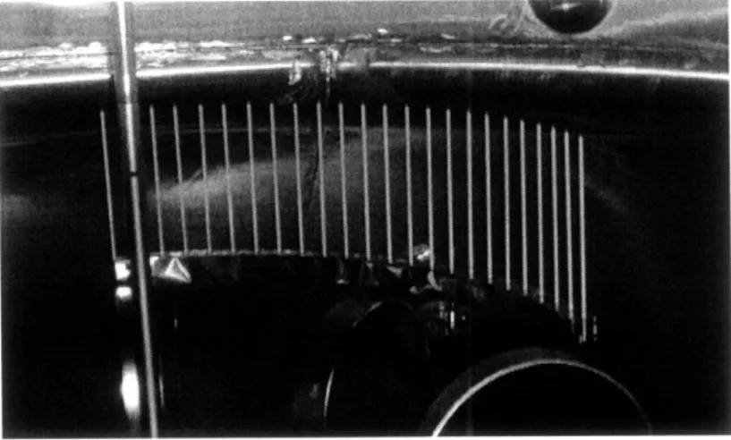
1.3

Electrostatic Probe Array

The electrostatic probe array is composed of twenty-four cylindrical, tungsten-tipped floating potential Langmuir probes. The array is positioned at a radius of one meter and sweeps out a ninety degree arc at the bottom of the LDX vacuum vessel. This

gives a probe separation of about 7 centimeters, giving the array a resolution of 14 centimeters. This resolution corresponds to a detectable mode number range of 1 to 46. The flow velocities arising from E x B drifts can be measured by computing the electric field from the plasma potential, and the energy cascades computed from the evolution of the spatial wavenumber spectrum.

Chapter 2

Theory

2.1

Probes

Langmuir probes are tools that measure the electrical characteristics of plasmas, and are among the oldest and simplest kinds of plasma diagnostics. In a general sense, a probe is simply an electrode placed within the plasma, as figure 2-1 shows. To get a local measurement, they are shielded from the plasma by a non-conductive material with a high melting point, typically a ceramic. Some types of probes simply measure the potential the electrode develops while in the plasma, others bias the electrode to a fix potential and measure the current drawn by it, and still others apply a time-varying potential to measure the whole I-V characteristic curve of the plasma. The probes in the LDX probe array are the floating potential variety, meaning they have a large resistor in series with the electrode. This is done to keep the current flowing in the probe low so that the electrode "floats" up to a potential called, surprisingly, the floating potential.

Figure 2-1: Schematic of a Langmuir probe.

2.1.1

Floating Potential

Ideally, the probes would measure plasma potential directly, but since they are not completely transparent to the plasma, they perturb the local environment they are placed in. An ideal probe draws no current, but even so it is not at the same potential as the plasma. This is due to the mass difference of the ions and electrons. Assuming their temperatures are equal, the electrons have a much higher velocity than the ions due to their smaller mass. Therefore, an electrode placed in the plasma would collect many more electrons than ions and emit a net current. Since the ideal floating probe does not allow current to pass through it, the current causes the electrode to charge up to a negative potential until sufficiently many electrons are repelled to equalize the rate at which ions and electrons are collected [10].

V = Vf + Te in 2x V + 2.5Te (for a deuterium plasma) (2.1)

The floating potential is related to the plasma potential by equation 2.1, where T is the electron temperature, Vf is the floating potential, V, is the plasma potential,M is the ion mass, and m is the electron mass [17]. In LDX, the electron temperature is approximately 25 eV, so the plasma potential is really about 75 volts higher than the measured floating potential. However, since its is an additive term, it does not affect the analysis of the fluctuations or the magnitude and direction of the electric field.

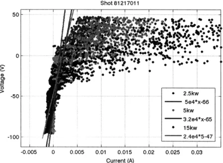
The potential measured directly from the probes is also not the floating potential. The probes are not ideal and draw a small amount of current. The current drops the measured potential from the actual floating potential as if there were another resistor between the probe tip and the floating potential. To get the real value of the floating potential, the slope of the linear region of the plasma's I-V curve (the plasma resistance) must be known. There are other probes in LDX that "sweep," i.e. they are driven with a certain potential waveform and the current flowing in the probe is measured. This way, the I-V curve of the plasma can be measured with a single probe while only sacrificing time resolution. As long as the plasma is relatively constant during the sweep period, the measurement is valid and can still measure time changes that take longer than a sweep period. To get an idea of the typical size of the resistance in LDX, a swept probe signal was taken from shot 81217011 and the slope of the linear portion was taken to be the resistance. The portion of the curve at higher voltages corresponds to "electron saturation," where the the electrons being drawn into the probe start repelling ions as well as creating

a current, and the net current formed departs from linearity. This shot was chosen since it was a "wedding cake" shot in that it uses all of the heating sources in different configurations. First 2.5KW of 2.45GHz ECRH was turned on, then 2.5KW more of 6.4GHz, and then 10KW more of 10.5Ghz for a total of 15KW. The resistance decreases with more heating, and has a maximum value of about 5.4 KQ2 for cooler

plasmas. With this resistance, Vpasm/Voat Rprobe (1M+lOk) = 995.

plasmaVfloat Rprobe+Rplasma (1M+10Ok)5.4k

This is a multiplicative correction, so it can affect the magnitude of the fluctuation and electric field measurements. Therefore, it is important to keep its value close to one. The resistor in the probe was chosen to be much larger than the plasma resistance, so that the multiplicative term is close to one and the floating potential can be closely approximated by the measured potential.

Shot 81217011 5 . .. .* ... .. .. . .. .. .* -- * S * *. -50 2.5kw | 5e4*x-66 * 5kw 3.2e4*x-65 * 15kw -100 - .-. 2.4e4*5-47 -0.005 0 0.005 0.01 0.015 0.02 0.025 0.03 Current (A)

2.1.2

Frequency Response

The probes need to measure potential fluctuations, so their response time must be faster than the regime of interest. Having a very large resistor in the probe is

problematic if it causes the RC time of the probe to become unacceptably large. Placing the resistor close to the probe tip reduces the capacitance of the probe, but there is still a small amount of capacitance associated with the sheath and the cabling. The capacitance of the sheath is 0.13pF as by equations 2.2 and 2.3 [11] [4]. AD is called the Debye length, and is the characteristic length for which perturbative effects from te probe take place. The coefficients a and b in equation 2.3 depend on electron temperature, but the equation can be further approximated to only depend on the plasma sheath area As and the Debye length. The sheath area is the surface area of the probe if it had a radius about five Debye lengths, making the capacitance proportional to another characteristic length, As/AD.

AD = 2NT = 2.35 x 10- 5 Tk (2.2)

C(Vf) = a oA (2.3)

b - 4AD 5AD

Together with the sheath resistance of 5.4KQ, an ideal probe would have a re-sponse time of about 0.7ns or 230MHz. The capacitance of RF coaxial cable is about

30pF per foot, which typically has a grounded shield very close to the conductor. The

cables inside the array have no shields and enamel insulation and therefore should have much lower capacitances than equivalent runs of coaxial cable. The resistor is

less than two feet from the probe tip, so a very conservative estimate of the cable capacitance is IpF. Together with a series resistance of 1MQ, this gives the probes

a -3db rolloff at f-3db = 2 - 160KHz. This lower bound of the frequency knee

intrinsic to probe electronics is well above the digitization rate and the frequencies of interest, and therefore it will not affect the measured signals.

2.2

Inverse Energy Energy Cascades in Plasma

Fluctuations

Analysis done by Grierson, et. al. at Columbia University's dipolar plasma in CTX inspired similar investigations in LDX. In order to measure the energy cascades in LDX, a signal from a model plasma had to be made to test the analysis method. A set of equations have been written by Hasegawa and Mima to describe the turbulence found in magnetized, nonuniform plasmas that have an electron temperature much higher than the ion temperature, where the time scales are much longer than an ion cyclotron period, and the turbulence is high enough that the wave-particle iterations are negligible [8]. Their turbulence equations were used to create a synthetic data signal similar to turbulent plasma that has nonlinear wave-wave coupling effects. This signal was used to test the analysis methods explained in the next section.

They derived these equations to explain the broad frequency spectrum observed in tokamaks that couldn't be explained by weak turbulence theories which assume a small departure from linear eigenmodes (and therefore have strongly peaked spec-tra). The equations are similar to mass conservation in a fluid element, and are shown in equation 2.4 where n and no are the perturbed and unperturbed densities, respectively, wei is the ion cyclotron frequency, and VI is the gradient perpendicular to the magnetic field. Qualitatively, the equations state that the rate of change of the particle density in a fluid element plus the net movement of particles in and

out of it is equal to zero. The velocities vE and vp are the E x B and polarization

drift velocities, respectively. These equations assume that the only phenomena that transport particles are related to these two drifts, and that the parallel phase ve-locity is much greater than the electron thermal speed, making the parallel motion unimportant. Both drifts depend on electric field (the E x B being static and the polarization being time-varying), and therefore are tied to the plasma potential.

On + V -[no(VE + Vp)] = 0[8] VE = -v 1 X Bo/Bo2 (2.4)

1

8a

[at

Assuming the electrons follow the Boltzmann distribution, the relation n/no = e¢/T can be written by quasi-neutrality. It can also be shown that V -(nvE) = 0 by continuity [8]. Expanding equation 2.4 in a Fourier series gives equation 2.5 [8].

00k(t) 1 at ZWk (t) 2 -)+

Z

/ax

Hasegawa and Mima also cover the consequences of this model, saying that that the mode coupling will rotate the plasma in the plane perpendicular to the mag-netic field. They also mention that large potential amplitude convective cell modes were directly excited by drift-wave turbulence in their computer simulations. This suggests that convective cells not only coexist with turbulence characterized by the Hasegawa-Mima equations, but could be powered by it. Due to their similarity to

the Navier-Stokes equations, the Hasegawa-Mima equations could lead to an inverse energy cascade that concentrates energy into low wavenumbers [8], and will obey Kraichnan's power laws shown in equation 2.6 [9].

E(k) = CE2/3k - 5/a

E(k) = C'r2/3k-3

In Kraichnan, 2D turbulence is shown to conserve kinetic energy and the mean-squared vorticity (vorticity = Q = V2E, where E is the stream function [18]), called enstrophy. From this, the power laws in equation 2.6 were derived [15], where

C _{and C' are dimensionless constants and e and T are the rates of cascade of}

en-ergy and enstrophy per unit mass, respectively. The k- 5_/3 _{power law corresponds to} a "downward" energy cascade where E < 0, i.e. that energy is transferred from the wavenumbers where this law holds to smaller wavenumbers with zero transference of enstrophy. The k-3 _{power law corresponds to an "upward" cascade in enstrophy,}

and zero transference of energy. These regimes can occur in the same spectrum, and cause energy to be transported to small wavenumbers and vorticity is transported to high wavenumbers. The downward cascade of energy implies that if high wavenum-bers are excited externally, their energy will be transferred to lower wavenumwavenum-bers. This gives the plasma a "self-organizing" characteristic that will cause energy from high modes excited by heating to move to large-scale structures in the plasma [15]. If the LDX plasma has these regimes, it is another indicator of fluid-like 2D turbulence and an inverse cascade of energy.

2.3

The Ritz Bispectral Method

The method derived by Ritz, et. al., is used to determine the direction, magnitude, and coupling of the energy cascades in the LDX plasma. The method assumes a stationary state, i.e. the power spectrum is unchanging. This implies that the linear growth rate of each mode is balanced by the energy transfer from nonlinear wave-wave coupling. It also is only accurate for systems where the majority of the power is in the linear and quadratic terms described by the wave coupling equation in equation 2.8. If incoherent or higher-order terms make up a large portion of the power, the computed transfer coefficients will not be accurate [21]. This equation is identical in form to equation 2.5, showing that this method is valid for characterizing the interactions that arise from the Hasegawa-Mima turbulence. The Hasegawa-Mima equations were derived for tokamaks, however, and are not directly applicable to a dipole plasma. They are useful to create a synthetic signal to test the the analysis routines using the Ritz method, as will be shown later.

0(k, t) =

3

k

00(k, t) = ALO(k, t) + A (k, k2)4(k, It)(k 2, t) (2.8)

at 2 kl,2

Ak = (7k + iwk) (2.9)

The first step in deriving the method is Fourier transforming then replacing the differential in equation 2.8 with the finite difference shown in equation 2.11. A finite difference is basically replacing the partial derivative with the definition of a derivative. The finite difference approximation of the partial derivative is only valid

for functions of 0 with slowly changing phase over the time interval 7 [21]. 0(k, t) = I(k, t)Iee(k,t) 84(k, t) = l( I ( k, t + 7)J - I(k, t)l 1

at

+i(kt)

)

If the Fourier transform is represented in magnitude and phase in complex no-tation as in equation 2.10, substituting equation 2.11 into equation 2.8 yields an

approximation to the wave coupling equation shown in equation 2.12.

(, ) A + 1 - i(|O(k, t + 7)J -

IO(k,

Redefining a few quantities gives a neat expression show in equation 2.16. The quantities Lk and Qkl,k2 are the linear and quadratic transfer coefficients, respectively. They characterize the linear and quadratic processes of the system and in conjunction form the "black box" system that modifies an "input" signal Xk to produce an "output" Yk.

Xk = 0(k, t), Yk = 0(k, t + 7) (2.13) Lk AT + 1 - i((k, t + T) - (k, t)) (2.14) Lk k -i((k,t+7)-(k,t)) (2.14) AQ(ki, k2)7 Qk = _{ek _i(e(k,t+r)-(k,t))}( k2)T (2.15) Yk LkXk + I E QkYkXk,Xk 2 (2.16) ki,k2

This system is not directly invertible, and more involved methods must be used to obtain the transfer coefficients from the input and output of the system. This is due to the nonlinear nature of the system desribed by Qkl,k2. To create a solvable set

of equations, moments are built from equation 2.16. The first moment is made by multiplying equation 2.16 by the complex conjugate of Xk and ensemble averaging (denoted by (...) in the equations) over many independent realizations. These ensem-ble averaged quantities are call "estimators" since the estimate the true value of the autopower, crosspower, bispectrum, et cetera by averaging many different instances of the same quantity. An individual measurement may be far from the true value, but averaging over many should make the value converge to the true value. Its like computing the temperature of a material by measuring and averaging the kinetic energy of individual molecules.

(YkXk) = Lk(XkXk) + Qk,k 2 (XkXkiXk2) (2.17)

k ,k₂

(YkX,X, = Lk (XkXk X ) + E Qklk2 (Xk X~ X klX k2) (2.18)

The second moment equation is made by multiplying by X*, _k1 X*, _k2and ensemble averaging. This produces the fourth order moment (X*, X *,XkiXk2), which is a

very computationally intensive quantity to compute, so a closure approximation is made assuming all off-diagonal terms (k', k) 4 (k1, k2) are zero. Approximating (X*,X ,XkXk 2) with the second order moment (XXkXk2) is called the

Million-schikov approximation [21]. This approximation causes the summation in 2.18 to drop out, and the quadratic transfer coefficient can be directly extracted from the equation [21].

The transfer coefficients are the only unknowns in the two coupled moment equa-tions and thus can be solved for. The transfer coefficients are given by quantities shown in equation 2.19. They can be solved iteratively by using an initial guess for Lk where Qkl,k2 = 0. The equations should be self-consistent and converge onto the

proper transfer coefficient values for a given set of estimators [20].

(YkXZ) - E Qkl,k2 (X XkXk 2)

kl>k2 (YkXklXk2) - Lk(XkXkXj 2.19)

Lk - klk2 12k .X2)19)

(XkXk) 2 (IXklXk₂ 2

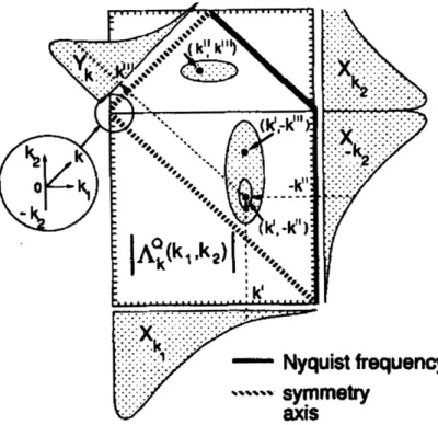
To determine the direction on magnitude of the power transferred between cou-pled waves, the coupling coefficient, AQ (k, k2) (which is equal to the transfer coef-ficient multiplied by the phase shift, which can be approximated by equation 2.23 [21]), is multiplied by the bispectrum and the real part is taken (shown by the "R" operator). This new quantity is called the quadratic power transfer coefficient, and is shown in equation 2.21. When it is plotted, the negative regions show the wavenum-bers that have power being drawn out of them into waves with smaller wavenumwavenum-bers. Positive regions show the converse, or wavenumbers that have two smaller

wavenum-bers putting power into them. Figure 2-4 shows an illustration of this three-wave breakdown/buildup process. By summing along all contributions to a single k, a quadratic power transfer function similar to the linear growth rate (eqn. 2.20 [13])

can be computing from Tk, as shown by equation 2.22. These plots are shown in the results section, and represent the net power transferred into a wavenumber, k, from positive and negative contributions (buildup and breakdown) of other wavenumber

pairs, k1 and k2's [21]. S= - 1 _(2.20) T T (kl, k2)= R(AQ(kl, k2) (klklk 2)) (2.21) k= ZT (k, k₂) (2.22) k ,k2 e-i(o(k,t+_)-e(k,t)) (YkX) (2.23)

Ritz deals with the spatial spectra, but the method can be applied in both time and space. If temporal frequencies are examined, the signals need to come from two probes separated in space. In a mathematical sense, the spatial method com-pares many 0(k, t) and 0(k, t + 7)'s, whereas the temporal method comcom-pares many O(x, w) and O(x + Ax, w)'s. If spatial frequencies are examined, the signals need to come from a probe array signals separated in time. The majority of the analysis done here deals with the spatial application of the Ritz method since the probe array allows direct measurement in wavenumber space. The plasma is assumed to rotate, however, and there should be a relation between the wavenumbers and frequencies shown in either analysis. I will discuss the time method first since the routines were tested with "time-like" synthetic signals. It is easier to create synthetic time

sig-- Nyquist frequency

--

symmetry

axis

Figure 2-3: Graphical description of how the quadratic coupling coefficients relate to the input and output signals taken directly from Ritz. The figure shows how a set of wavenumbers that satisfy the condition k = ki + k2 are multiplied by the value of Qk(kl, k2) and summed to produce the resultant value of k. It highlights the areas of the coupling coefficient like lines of constant k, Nyquist cutoffs, and symmetry axes. [21]

Power

k, k

k2

Power

Figure 2-4: Illustration showing how the three waves interact depending on the sign

nals and this is the only reason it was tested in time rather than in space. If the algorithms are valid for time analysis, they should also work for space since the only difference between the two is along which dimension the Fourier transform is made. The method in time space starts by taking the fast Fourier transform (FFT) of the two input signals and normalizing (dividing) the transform by its length. These two signals are offset by a distance Ax in space. The signal is assumed to have gone through a linear and non-linear change described by a "black box" operation during the distance Ax, shown in figure 2-9. The input to the black box is the signal measured at x and the output is the the signal measured at x + Ax. From these two long time signals, small samples are taken at equal times and used to compute the estimators. The window is then moved down the signal and the estimators are recomputed. Figure 2-5 shows this process diagrammatically. The set of estimators acquired by this process make up the ensembles used to compute the ensemble averaged estimators and ultimately the transfer coefficients.

Signal x

Previous windows Fourier Transformed t compute (..) quantities

.. ... .. ... .

Signalx+A x

Figure 2-5: How samples are taken from two time signals to make ensembles.

To test the method, a synthetic signals had to be made where the linear and quadratic transfer coefficients were know a priori. Such a signal set was created by using Fourier transformed Gaussian random noise to excite the "black box" system described by equation 2.16 then inverse Fourier transforming the input and output

signals back into time. A large number of points had to be used in constructing the signal so sampling the signal in time with a moving window would produce a reasonable approximation. The ideal signal is continuous, so the appropriate length the synthetic signal needed to be was determined by sampling theory.

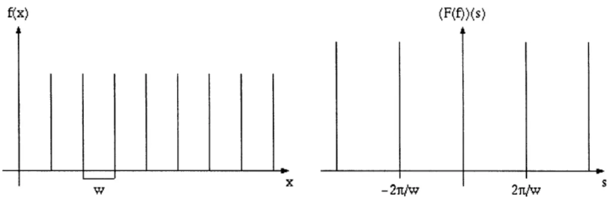
Sampling can be thought of as multiplying a function with a Dirac comb function. Since multiplication in normal space is convolution in Fourier space, sampling a signal with a finite Dirac comb is the same as convolving its frequency spectrum with the transform of a finite comb. The Dirac comb is simply a train of Dirac delta functions, and its Fourier transform is a complex exponential. Since the Fourier transform is a linear operator, the Fourier transform of a finite comb is simply a sum of harmonic complex exponentials with the fundamental at the sampling width, T, and the last harmonic at half the sample points, Ny, as shown in equation 2.24. The sum of complex exponentials converges to a dirac comb function with spacing 2, shown in figure 2-6. For the signal to be perfectly reconstructed in frequency space, the width of the frequency space comb must be twice as wide than the highest frequency present in the signal (the Nyquist sampling theorem).

comb = 6(x - nT) + COMB = ei k n T _(2.24)

n n

If this condition is satisfied, then the convolution will produce a train of spectra that do not overlap, i.e. every frequency is perfectly resolved. The effect of trun-cating the comb in normal space is that the sum of sine waves in frequency space is also truncated, and therefore the sampling kernel is not a perfect Dirac delta. The resulting pseudo-delta has some finite width from truncation, and smears out the details of the frequency spectrum when the signal is convolved in frequency space. Figures 2-7 shows the sampling kernels corresponding to sampling in normal space

(F(f))(s)

w -2n/w 2n/w

Figure 2-6: The Dirac comb function and its Fourier transform [161

with a truncated Dirac comb. Since adding points in normal space is the same as adding additional terms to the sum in frequency space, adding two additional points in normal space is the same as adding one harmonic term in frequency space, so the first harmonic corresponds to 3 points, the second to 5 points, etc. Figure 2-8 illus-trates the effect of sampling on a slightly noisy signal. The lower harmonics average over the signal by their FWHM. Using smaller windows effectively smudges out the details in the spectrum, and therefore shorter time series can be used to construct the synthetic signal if small windows are used to sample it. If wide windows are used, the imperfections in the construction will become apparent and will no longer look like the coefficients used to construct the signal. A fit to the FWHM trends of the sampling kernels yields FWHM = 2.126/x-7 493 where x is the harmonic number

(or x= samples-1

The experimental data has a width of 22 points (since the first and last channels were broken on installation), but is padded up to 92 points, so the analysis was tested with a window of 92 points. Using a very conservative 100 signal widths within one

window width, a synthetic signal width of 8_{signal =}

74 100(Ssample - 1)+ 1 45, 000

was determined. This fact was important for computing the test case since running

the signals through the quadratic sum in equation 2.16 takes many hours to run. This in mind, the test case was done using the temporal method since only two long signals needed to be created. To directly test the spatial method, many consecutive signals needed to be made, and doing so for signals of this length would have taken months of computing time. Using the temporal method to test the code apposed to the spatial method should still give an indication if the code is working as it should.

Figure 2-7: Progression of sampling ker- Figure 2-8: Effect of finite sampling in nels as more points are added in time. time on frequency spectrum construction.

The test signal was made by feeding 150,001 Gaussian random points (to ab-solutely ensure accuracy) through 5 black box nonlinear systems in series, and the input and output of the fifth box was used to test the analysis routines. The transfer coefficients used are shown in equation 2.25 and resemble the the form of the coeffi-cients in the Hasegawa-Mima equations in equation 2.5

[20].

.. .. .. ... ... ... ... ... "... . .. . ..T.... ... .. ... ... .. ... ... ...

of the window width. The overlap introduced phase changes large enough to enhance_{... ...}

. ... ... ... .. .. ."...

i" . ... .. ... . .. ...

-1*. 4... ..... .e .4 .. ..

Figure 2-7: Progression of sampling ker- Figure 2-8: Effect of finite sampling in nels as more points are added in time. time on frequency spectrum construction.

The test signal was made by feeding 150,001 Gaussian random points (to ab-solutely ensure accuracy) through 5 black box nonlinear systems in series, and the input and output of the fifth box was used to test the analysis routines. The transfer coefficients used are shown in equation 2.25 and resemble the the form of the coeffi-cients in the Hasegawa-Mima equations in equation 2.5 [20]. Ensembles were built by moving a window of 92 points across the time signal with an overlap of one-sixteenth of the window width. The overlap introduced phase changes large enough to enhance convergence of the ensembles. This method is useful for determining the coupling between the frequencies in LDX assuming the turbulence is well-characterized by the

Hasegawa-Mima equations and there are very few iterations other than linear and quadratic. Figure 2-9 illustrates the evolution of the random signal into the signals used to test the analysis. The input coefficients used to calculate the test signal are shown in figures 2-10 and 2-11. The curvatures of the linear and quadratic coeffi-cients are in opposition so the system tends to an equilibrium spectrum where the two growth rates sum to zero.

k2 _k Lk(k) = 1 - 0.4 k2 + i0.8 k Nyquist _kNyquist i kik2(k_{2 -} k2 (2.25)) Qk(k, k2) ₄ 2 Nyquist 1 + k2/kNyquist Noise L(k) k L(k) L-pectru klk21 k2 k1l, 1 1,k2 Spectru kl,k2 Q kl,k2 klk2 Q k1,k2) Xk 1 Yk1 Yk 2 k

Figure 2-9: Block diagram analogous to taking temporal measurements showing the modification of an input signal by five series block box systems (top), and a diagram analogous to taking spatial measurements showing the modification of an input signal another series block box systems (bottom).

In the analysis, negative wavenumbers do not imply wave propagation in an op-posite direction, they simply give an alternate amplitude and phase that can describe an identical wave as the positive wavenumber value. Therefore, including the nega-tive wavenumber space allows all possible combinations of three wave iterations to be considered.

1.0 _0.064 0.8 0.056 0 0.048 0.4 0.040 0.2 0.032 4 0.00 -0.2 0.024 -0.4 _0.016 -0.6 _Real 0.008 - .0 -0.5 0.0 0.5 1.0 _0.000 k 0.00 0.17 0.33 0.50 0.67 0.83 k1

Figure 2-10: Linear transfer function used _{Figure 2-11: Quadratic transfer function}

to produce the synthetic data _{used to produce the synthetic data}

i.e. Qk(kl, k2) = Qk(k 2, kl), only the non-redundant quadrants where kl _{k2 are}

plotted in the following figures. The axis of symmetry is shown by the green dashed line and the Nyquist limit by the red dashed line. The "upper triangle" is limited by the Nyquist condition in k and the "lower triangle" is limited by the Nyquist condition in kl and k₂.

The plots show that the analysis routines can indeed measure the quadratic and linear transfer coefficients since the simulated and analytic coefficients have good agreement. However, the analysis carried out in most of this thesis will be the spatial kind since the probe array was constructed to directly measure spatial fluctuations. These measurements can be compared to similar temporal ones to ensure agreement or to point out interesting differences.

Shot synthetic data, 0 to 150,000 points

Ouadratic Transfer Function. IO(kl,k2)1

Linear Transfer Function, L(k)

Ouadratic Power Transfer Function, T(kl,k2)

0.064 0.056 0.048 0.040 0.032 0.024 0.016 0.008 0.000 0 8 6 4 .2--Real .6 ... ... ...I a y r - - 0 20 4 -40 -20 0 20 40 n

Quadratic Power Transfer

10 20 30 40 13.00 0 -10000 -20000 -30000 -40000 -50000 -60000 -70000 0.000025 0.000020 0.000015 0.000010 0.000005 0.000000 -0.000005

Linear Growth Rate

. ... ... -.... ... ... ... ... ... ... ... ... .... : ... ... i ... ... ... ... ... ... ... ... ... ... ... .. ... ... ... ... ,... ... ... ... ... ... ... ... !... i... .. .... ... ... .. -17.0 -27.0 -37.0 1. 0. 0. 0. 0. 0. -0 -0 -0 -n 0 40 0.05 0.04 0 .0 3 ... ... . ... 0 .0 2 ... ... .. ... ... :. .... ... 0 .0 1 ... ., ... ... .. ... 0.0 0.01_{0.0 10 20 30 40}

Figure 2-12: Quadratic and linear transfer functions, linear growth rate, quadratic power transfer, and power spectrum compted from the synthetic test data.

0 0 0 10 20 3 n Power Spectrum 0.00015S 0.00010 0.00005 0.00000 0.00005 0 .n I I I i """"'' |||||| |1|1 0 / , ... .. . . . . . . . . . . . . ... .. ... . .. . . .. . . .. .. .. . . .. . .. . . . .. . . .. . . . . .. . . ... ... ...

2.4

Phase Velocity, Drifts, and Wavenumber

Spec-trum

The data collected by the probe array can be used for more direct analysis than the Ritz bispectral method. The plasma rotation speed can be calculated directly from stripey plots, which simply plot the probe fluctuation amplitude versus time. The phase speed is simply the slope of the line when the probe number is scaled to distance. If the plot is extended to 27, or 92 probes, the mode number in the plasma can also be determined by the number of times a line on the stripy plot overlaps itself. Since the array spans ! radians, the resolution spectrum created by taking the FFT of the 22 data points is only 4 mode numbers, despite having a Nyquist frequency at n=46. Most of the phenomena of interest is at low-frequencies, so the resolution of the signal is increased by padding the input signal from the array to 92 points (which corresponds to 27 radians) with zeroes. This way, the FTT has a resolution of 1 mode number and each mode can be distinguished. Padding is in essence the same as interpolating the stripey plot to determine the mode numbers.

E= -Vb (2.26)

B 2 (2.27)

Uplasma = R a (2.28)

The wavenumber power spectrum itself if also of interest, and can be measured by averaging the autopower spectrum, (XkXk), over a time interval. From this, it can be measured if the spectrum obeys the power laws stated in Kraichnan, and if

it is suggestive of inverse energy cascades. The dominant modes are also easily seen from the power spectrum, and determining their common values and relation to the frequencies present is important information.

Since the potential is measured by the probes, the azimuthal/toroidal electrical field can be directly determined from the gradient of the potential as shown in equa-tion 2.26 [7]. The elctric field can be used to compute the E x B drift velocity, as shown in equation 2.27 [4] . These drifts are directly related to convection, and measuring their magnitude shows its strength in transporting particles to and from the core of the plasma.

Chapter 3

Experimental Setup

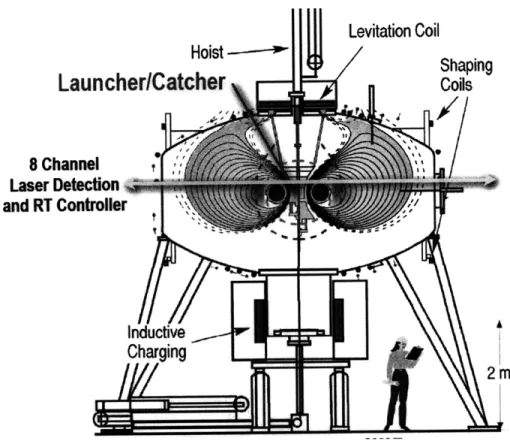
The LDX vacuum vessel is a large, puck-shaped, half inch thick stainless steel cham-ber. It has is three meters tall, 5 meters in diameter, and has a volume of about 65 cubic meters. High vacuum is established in the chamber by means of turbo- and cryo-pump systems. Figure 3-1 Shows a cutaway of the vacuum vessel and highlights the main components of LDX.

The magnetic dipole field is created by the floating coil, or "F-coil," which is levitated in the center of the vacuum chamber during plasma shots. Levitation clears the path inside the coil ring, and allows particles to move freely along the entire field line. This reduces particle losses and improves confinement times. The F-coil must be able to stay levitated for an extended period of time and cannot have any external connections to keep current flowing in it. Therefore it is made of the low temperature superconducting material Nb3Sn and be charged inductively. The

F-Coil weighs 565 kg, is cooled with helium, and can remain superconducting for up to 2.5 hours [1].

Hoist

--LauncherlCatcher

Levitation Coil

4

8 Channel

Charging

2m

Figure 3-1: A cutaway of the Levitated Dipole Experiment. This view shows the floating coil in the center of the vacuum vessel, levitation coil on top of the vessel, charging coil inside the charging station underneath the vessel, launcher/catcher, and laser position system.

vacuum vessel. This coil is called the charging coil (C-coil), and is made of another low-temperature superconductor, NbTi. The warm, non-superconducting F-coil rests inside the C-coil prior to charging while the C-coil is charged to 425 amperes (3.6 MA-turns). Then the F-coil is cooled with helium, which makes it superconducting, and the C-coil is discharged. This causes current to flow in the F-coil. The F-coil is then raised to the middle of the vacuum vessel mechanically. A third, copper coil on top of the vessel is turned on to levitate the F-coil, and its mechanical supports are backed away. At this point, LDX is ready to make plasmas [1].

Plasmas are made by releasing a small amount of gas (deuterium or helium) into the vessel before high power microwaves are injected. The microwaves ionize the gas by means of ECRH (electron cyclotron resonance heating), where most of the power is absorbed by electrons that have a cyclotron frequency the same as the microwave frequency. The microwaves therefore heat the plasma at shells of constant field strength. The microwave powers and frequencies using in LDX are 2.5 kilowatts of 2.45GHz, 2.5 kilowatts of 6.4GHz, and 10 kilowatts of 10.5GHz. The microwaves themselves are weakly attenuated by the plasma, so they bounce inside the vessel many times before being dissipated. By this reflection mechanism, the microwaves heat the plasma isotropically [1].

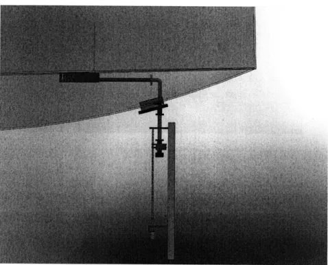
The probe array enters the vessel through a port on the bottom southwest side of the vessel. The tips of the probes are at a constant 1 meter radius, and can be positioned from -65cm to -45 cm from the midplane. Figures 3-2-3-4 show the posi-tion of the array with respect to the floating coil and the magnetic fields. The probe is usually positioned close the the "seperatrix" during plasma shots. "Seperatrix" is another word for the last closed field line. Inside the seperatrix, particles can stream along a field line without being lost. Outside the seperatrix, field lines intersect ob-jects, and a particle streaming along a field line is almost immediately lost. Figures

Figure 3-2: Top-down view of LDX's midplane showing the position and extent of the probe array are.

r (cm)

Figure 3-3: The probe array position rela-tive to the field lines at the separatrix. The red line shows the direction of the mag-netic field at that point. The ExB direc-tion measured by the array is at a right angle to the red line, pointing radially in-wards. The blue line shows the field line intersecting the probe tip.

Figure 3-4: The probe array position rela-tive to the field lines at full insertion. The red line shows the direction of the mag-netic field at that point. The ExB direc-tion measured by the array is at a right angle to the red line, pointing radially in-wards. The blue line shows the field line intersecting the probe tip.

3.1

_{Probe Array Design}

Figure 3-5: SolidWorks model of the entire array system.

3.1.1

Mechanical

Construction

The floating potential probes alumina ceramic tubes with long tungsten tips. The ceramic has 16 inches of exposed length from the top of the array arc. This length was chosen so the tips are 10 cm out of the separatrix when fully extracted (the array hits the bottom of the vessel).

The positioning of the probe array is critically important since the plasma fluc-tuations under investigation occurs near the edge. The probe tips are one centimeter of exposed 0.125 inch diameter, 2% thoriated tungsten, which required them to be

Figure 3-6: The probe array installed in the LDX vacuum vessel.

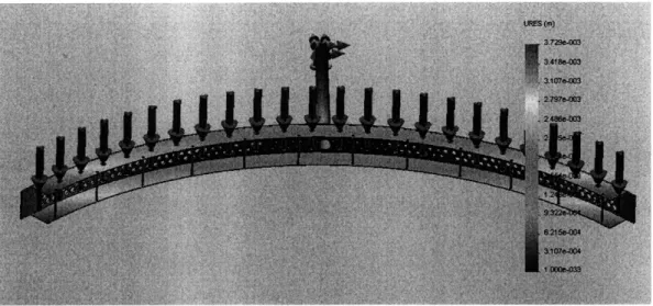
placed at a position with half centimeter accuracy. The structure of the array arc was designed to keep the probe tips positioned accurately by reducing lever arm errors due to the flexing of the support materials under gravity.

SolidWorks was used to simulate the probe array structure under gravity. A box-like structure was initially attempted to create a rigid arc without much weight. This designed was improved upon by making the back wall 0.3185 inches thick, the top and bottom walls 0.109 inches thick, and cutting out a pattern of holes in the back wall. The circular holes have a hexagonal distribution and an area that increases exponentially approaching the ends of the arc. Less weight is supported further out , so less material is needed to support it. Using this pattern greatly reduced the total weight of the structure without sacrificing much strength, and therefore reduced the amount of flexion it experiences under gravity.

Since there needs to be access to the wiring in order to swap probes, the front edge of the array arc is supported by 0.25 inch diameter tubes instead of a large plate. This allows easy access to the array internals while keeping the structure rigid and reducing total weight. A 20 mil plate of 316 stainless steel was placed over the

Figure 3-7: A probe tip.

Figure 3-8: The PEEK insulator and solid copper conductor.

front to protect the wiring from the plasma. This plate is tack welded so it could be easily removed if access is needed.

The probes are held into the array arc by stainless steel holders like that shown in figure 3-10. The holders are welded to the bottom of the arc's top plate and use set screws to secure the probes' ceramic housing to the arc. There is a set screw in the PEEK insulator at the bottom of the holder which fixes the length of tungsten electrode protruding from the probe tip while keeping the conductor electrically isolated. The copper conductor is passed out through the holder's bottom and is terminated in a pushpin connector. A 1 megaohm resistor is connected in series with the conductor with similar pushpins and sockets for easy removal. The resistor is connected to a socket clamped into a ceramic terminal block which is hardwired to the a 32-pin vacuum feedthrough.

Figure 3-9: Closeup of the probe array 'K MW J without the front shield. This view clearly

shows the cutout pattern of the back rib, Figure 3-10: Detail of the probe holder the probe holders, the front braces, and and terminal block highlighting the

resis-the ceramic terminal blocks tor and connection pins/sockets.

Movement

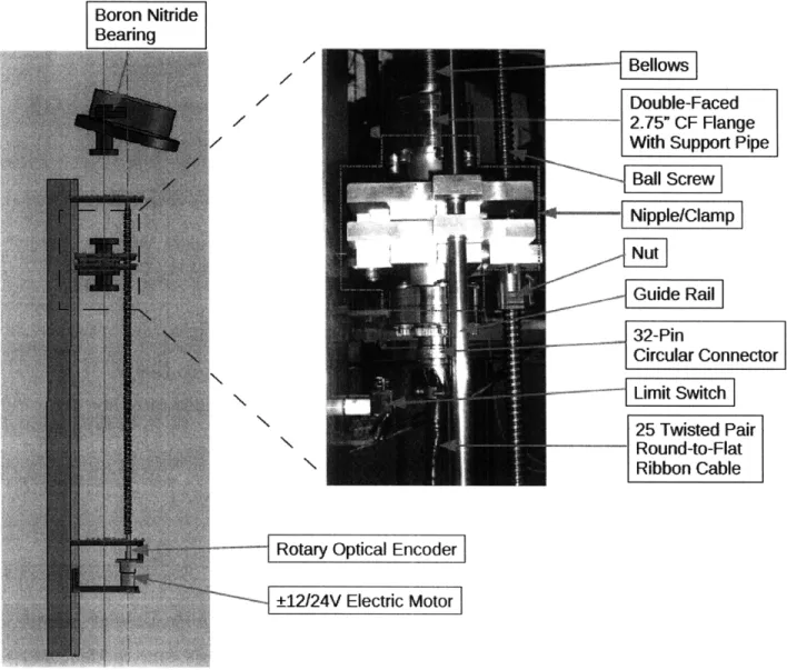
The probe array's drive system is composed of a ball screw attached to a vacuum nipple that rides on two rails. The ball screw drive is 98% efficient at converting rotational to linear motion, and allows a small Pittman GM9413-2 electrical motor to power the system. This motor provides a maximum continuous 45 oz-in of torque with 0.6 amperes of current and 65 rpm. The probe array pipe is connected to the drive system by a double-faced flange welded to its bottom. This flange has a full nipple above it and the 32-pin electrical feedthrough below it. A machined aluminum clamp holds the nipple to the rails. Above the nipple is a custom edge-welded bellows that keeps vacuum while allowing the array to move. This bellows has a compressed and extended length of 20 and 70cm, respectively, for a total travel of 50 centimeters. The pipe is preventing from rubbing against the vessel by a boron nitride sleeve bearing welded to the back of the vessel flange. This bearing also

Figure 3-11: SolidWorks simulation of the probe array. Colors show the amount of deviation from a perfectly rigid model. Maximum deviation is 1.6mm.

relieves the torque put on the weld in holding the pipe upright. The entire assembly is mounted to the vessel by a large aluminum channel. This channel is screwed to gussets that are welded onto the vessel itself. Figure 3-12 illustrates how the various components of the drive system connect to each other.

Automation

The vertical position of the probe array is remotely controlled by a programmable logic controller (PLC) system. A Rockwell Automation/Allen Bradley MicroLogix 1500 PLC was installed at LDX prior to the probe array's construction, and was modified to control the probe array in addition to the other probes it controls. A 1769-HSC high-speed counter module was added to the PLC to count the pulses from an optical encoder and determine the array's position. The Dynapar M151000/8291A optical encoder sends 1000 pulses per revolution of the ball screw and has three channels of quadrature which allow the counter to count forward backward. The