Sampling and condition assessment of ductile iron pipes

(1)

https://doi.org/10.1061/41173(414)4

READ THESE TERMS AND CONDITIONS CAREFULLY BEFORE USING THIS WEBSITE.

https://nrc-publications.canada.ca/eng/copyright

Vous avez des questions? Nous pouvons vous aider. Pour communiquer directement avec un auteur, consultez la

première page de la revue dans laquelle son article a été publié afin de trouver ses coordonnées. Si vous n’arrivez pas à les repérer, communiquez avec nous à PublicationsArchive-ArchivesPublications@nrc-cnrc.gc.ca.

Questions? Contact the NRC Publications Archive team at

PublicationsArchive-ArchivesPublications@nrc-cnrc.gc.ca. If you wish to email the authors directly, please see the first page of the publication for their contact information.

NRC Publications Archive

Archives des publications du CNRC

This publication could be one of several versions: author’s original, accepted manuscript or the publisher’s version. / La version de cette publication peut être l’une des suivantes : la version prépublication de l’auteur, la version acceptée du manuscrit ou la version de l’éditeur.

For the publisher’s version, please access the DOI link below./ Pour consulter la version de l’éditeur, utilisez le lien DOI ci-dessous.

Access and use of this website and the material on it are subject to the Terms and Conditions set forth at

Sampling and condition assessment of ductile iron pipes

Kleiner, Y.; Rajani, B. B.

https://publications-cnrc.canada.ca/fra/droits

L’accès à ce site Web et l’utilisation de son contenu sont assujettis aux conditions présentées dans le site LISEZ CES CONDITIONS ATTENTIVEMENT AVANT D’UTILISER CE SITE WEB.

NRC Publications Record / Notice d'Archives des publications de CNRC:

https://nrc-publications.canada.ca/eng/view/object/?id=956b4531-c44f-405b-a8fb-d4e842da0e44 https://publications-cnrc.canada.ca/fra/voir/objet/?id=956b4531-c44f-405b-a8fb-d4e842da0e44

(2)

http://www.nrc-cnrc.gc.ca/irc

Sa m pling a nd c ondit ion a sse ssm e nt of duc t ile iron pipe s

N R C C - 5 4 4 3 7

K l e i n e r , Y . ; R a j a n i , B . B .

M a y 2 0 1 1

A version of this document is published in / Une version de ce document se trouve dans:

World Environmental & Water Resources Congress, Palm Springs, CA, USA,

May 22-26, 2011

The material in this document is covered by the provisions of the Copyright Act, by Canadian laws, policies, regulations and international agreements. Such provisions serve to identify the information source and, in specific instances, to prohibit reproduction of materials without written permission. For more information visit http://laws.justice.gc.ca/en/showtdm/cs/C-42

Les renseignements dans ce document sont protégés par la Loi sur le droit d'auteur, par les lois, les politiques et les règlements du Canada et des accords internationaux. Ces dispositions permettent d'identifier la source de l'information et, dans certains cas, d'interdire la copie de documents sans permission écrite. Pour obtenir de plus amples renseignements : http://lois.justice.gc.ca/fr/showtdm/cs/C-42

(3)

(4)

SAMPLING AND CONDITION ASSESSMENT OF DUCTILE IRON PIPES

Yehuda Kleiner and Balvant Rajani

National Research Council of Canada, Institute for research in Construction Ottawa, Ontario, Canada

Yehuda.Kleiner@nrc-cnrc.gc.ca Abstract

About 300 ft (91.4 m) of DI pipes were exhumed in each of four North American water utilities in an effort to gain a thorough understanding of the geometry of external corrosion pits in ductile iron (DI) pipes, which would lead to a better ability to assess the remaining life of these pipes. The exhumed pipes were cut into sections, sandblasted and tagged. Soil samples extracted along the exhumed pipe were also obtained. Pipe sections were scanned, using a laser scanner that was specially developed at the National Research Council of Canada (NRC) for this purpose and the scanned data were processed using special software developed for this purpose. The pipes were virtually sliced into rings of equal lengths, where each ring was characterized by three geometrical attributes, namely maximum pit depth, pit area and pit volume. Statistical analyses were performed on the geometrical attributes of the corrosion pits found on these rings. Soil characteristics were investigated for their impact on the geometric properties of the corrosion pits and were found not to have a substantial and consistent impact.

Based on the results of the statistical investigation, methods were proposed to discern the condition of a ductile iron pipe based on a set of random samples. In this paper we describe the development of these methods, including the sampling scheme, the probabilistic inference on the pipe condition and the confidence bounds for the discerned results.

Keywords

Corrosion pits, condition assessment, corrosion pit geometry, probability distribution, sampling.

1. INTRODUCTION

The National Research Council of Canada (NRC) and the Water Research Foundation (WRF – formerly known as AwwaRF – American Water Works Association Research Foundation) co-funded a research project to investigate the long term performance of ductile iron (DI) water mains. One of the sub-objectives of this research was to gain a thorough understanding of geometry of external corrosion pits and the factors (e.g., soil properties, appurtenances, service connections, etc.) that influence this geometry. It was hoped that this understanding would lead to the ultimate objective of achieving a better ability to assess the remaining life of ductile iron pipes for a given set of circumstances.

Four North American water utilities exhumed each about 300 ft (91.4 m) of DI pipes that were slated for replacement. The exhumed pipes were cut into sections, sandblasted and tagged. Soil samples extracted along the exhumed pipe were also obtained. Pipe sections were scanned, using a laser scanner that was specially developed at the NRC for this purpose and the scanned data were processed using special software developed for this purpose. Statistical analyses were performed on three geometrical attributes, namely pit depth, pit area and pit volume. Various soil characteristics were investigated for their impact on the

(5)

geometric properties of the corrosion pits. Kleiner et al. (2010) provided a detailed description of the acquisition of the data and presented results of the statistical analysis of the corrosion pits in the exhumed pipes. In this paper we describe how these results can be used to make an inference on the condition of a DI pipe based on pit properties of some discrete samples.

The paper is organized as follows. The second section provides a brief description of the data extraction and preparation as well as the statistical analysis of the corrosion pit data and a summary of the main

conclusions of this analysis. The third section describes the sampling schemes that were examined and compared for this research and the fourth section provides a description of the method proposed for making an inference about the pipe condition. Summary and conclusions are provided in the fifth section.

2. DATA COLLECTION, PREPARATION AND ANALYSIS

Only three data sets (of six) were complete enough to perform the statistical analysis described here (Table 1), and Kleiner et al. (2010) reported the results of two of those datasets (Calgary and Kansas City). The exhumed pipe was cut into sections of about 1.1 m (3½ ft) long. The exterior surfaces of these sections were sandblasted to reveal “corroded” or “graphitized” iron and subsequently scanned by a pipe laser scanner. The raw scanned data were processed and cleansed, using a six-step process as described by Kleiner et al. (2010). Soil samples were also extracted every 7.6 to 15.2 m (25 to 50 ft) along the exhumed pipes. These soil samples were sent to local testing laboratories to measure soil properties as suggested in AWWA C105/A21.5-99.

Table 1. Exhumed pipes details

City (Water utility) Diameter Depth length Installation year

Kansas City (Water One) 300 mm (12”) 1.07 m (3.5 ft) 91.4 m (300 ft) 1989

Louisville (Water Co.) 200 mm (8”) 1.07 m (3.5 ft) 91.4 m (300 ft) 1972

Calgary (Water Dept.) 250 mm (10”) 3.05 m (10 ft) 91.4 m (300 ft) 1969

Each of the exhumed pipes was virtually sliced into segments (or rings) of length x, where x = 25, 50, 100, 150, 300, 450 and 600 mm (approx. 1, 2, 4, 6, 12, 18 and 24 inch). Thus for example, an exhumed pipe of 10 m (10,000 mm) length would result in a population of 400 rings 25 mm long, or a population of 200 rings 50 mm long, and so on. This means that data for each exhumed pipe were examined seven different times with seven different ring populations. For each population, three pit properties were investigated, namely, the distribution of maximum pit depth in a ring, the distribution of the corroded surface area in the rings and the distribution of pit volume (wall loss) in the rings. Kleiner et al. (2010) described in detail the various (theoretical) probability distributions that were examined for fitting the observed pit data. Table 2 provides the results of this analysis for the Calgary data. As can be seen, the right-truncated Gumbel distribution was found to best fit the distribution of pit depth maxima. This boded well with theoretical expectations because the right-truncated Gumbel (truncated at the pipe wall thickness) is an extreme value distribution and the population at hand is indeed truncated. The Weibull distribution was found to best fit the distribution of pit area and pit volume populations. Due to space limitations, we focus in this paper mainly on Calgary data(one example relates to Kansas City data), but it should be noted that these results were similar to those obtained for the analyses of the Kansas City and Louisville data.

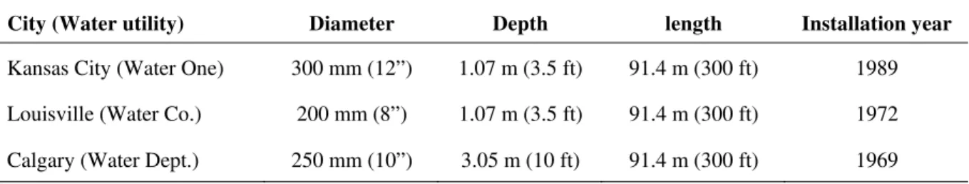
Figure 1 provides an example to illustrate the fact that dependency between soil properties (electrical resistivity in this case) and corrosion pit geometry (pit depth maxima in this case) was not visually obvious.

(6)

Table 3. Statistical analysis results of pit geometries in ring populations in Calgary* Ring Max. pit depth: trunc-Gumbel Pit area: Weibull Pit volume: Weibull Length (mm) Count Scale Location P-value Scale Shape P-value Scale Shape P-value

25 2297 1.45 1.41 0.000 13 0.29 0.000 21 0.27 0.000 50 1192 1.56 1.99 0.000 41 0.37 0.000 69 0.34 0.000 100 585 1.69 2.71 0.000 117 0.43 0.000 207 0.40 0.000 150 388 1.87 3.19 0.000 205 0.45 0.000 370 0.41 0.000 300 189 2.09 4.22 0.000 532 0.48 0.000 1008 0.44 0.000 450 83 2.06 4.59 0.007 824 0.47 0.001 1651 0.42 0.002 600 83 2.64 5.70 0.014 1289 0.51 0.002 2609 0.46 0.002 *Mean wall thickness (upper boundary for the truncated distribution) 8.44 mm.

The small dots in Figure 1 represent maximum pit depth in each ring (left axis) and the curve represents soil resistivity measure along the pipe (the markers on the curve are actual measured values in the soil samples and the curve represents interpolated (quadratic interpolation) values. Consequently, Kleiner et al. (2010) described in detail the statistical analysis applied to examine the impact of soil properties (and the presence of appurtenances) on corrosion pit geometry. A multi-covariate truncated Gumbel distribution was selected for pit depth maxima, where the location parameter (of the Gumbel equation) is a function of soil

properties: For the corrosion pit area and volume populations, a multi-covariate Weibull distribution was selected, where the scale parameter (of the Weibull equation) is a function of soil properties: The essence of this statistical analysis was to determine whether, and by how much soil property data, through

multi-covariate probability distributions, improve the ability to predict (or ‘explain’) observed variations in pit properties (maximum pit depth, pit area, pit volume) beyond the single-variate probability distributions. The likelihood ratio (LR) test was used to determine whether an additional covariate(s) actually improved the predictive ability of a model in a statistically significant manner. Soil properties that were examined included soil resistivity, redox potential, chloride, sulphide and/or sodium concentration, percent fines and soil pH. Each of these properties was considered in two ways, absolute values and rate of change

(derivative) values. In addition, the distance of a ring from an appurtenance was considered as well. Results indicated that a few soil properties had a statistically significant impact on pit geometry in a given city, but the impact of these properties was not always consistent within the dataset and between datasets. For example in Calgary, soil sodium concentration appeared to be the most consistently significant covariate, followed by the derivative of chloride concentration and proximity to appurtenances. In Kansas City, on the other hand, the derivative of sulphide concentration appeared to be the most consistently significant covariate, followed by %-fines and redox potential. In Louisville (not reported by Kleiner et al., 2010), derivative %-fines was the single most consistently significant covariate, however, when taken as a pair, soil resistivity together with absolute %-fines emerged as the most consistently significant pair of covariates. It was interesting to observe that soil resistivity, which in the literature is considered the most important factor to influence corrosion, emerged in this research as consistently significant only some times and even then only when paired with %-fines.

3. SAMPLING

The goal of this research was to draw statistical inference on the structural condition of a DI pipe, based on pit geometrical properties, coupled (possibly) with soil properties, both measured for a few sample rings along the pipe. As noted in the previous section, the data analyzed so far in this research provided no firm evidence that soil samples would always improve our ability to predict corrosion pit properties in any significant or consistent manner. Consequently, soil properties are not considered in our discussion of sampling and statistical inference on pipe condition.

(7)

Figure 1 Impact of soil resistivity (Ω•m) on maximum pit depth (various ring lengths) in Calgary data. 0 10 20 30 40 50 60 70 0 1 2 3 4 5 6 7 0 20 40 60 80 100 M a x pi t de pt h ( m m ) Length (m)

R

e

si

st

iv

it

y

80 90 100 8 9 600 mm rings 0 10 20 30 40 50 60 70 80 90 100 0 1 2 3 4 5 6 7 8 9 0 20 40 60 80 100 M a x pi t de pt h ( m m ) Length (m)

R

e

sistiv

it

y

0 10 20 30 40 50 60 70 80 90 100 0 1 2 3 4 5 6 7 8 9 0 20 40 60 80 100 M a x pi t de pt h ( m m ) Length (m)

R

e

sis

tiv

it

y

0 10 20 30 40 50 60 70 80 90 100 0 1 2 3 4 5 6 7 8 9 0 20 40 60 80 100 M a x pi t de p th ( m m ) Length (m)

R

e

si

st

iv

it

y

300 mm rings 100 mm rings 50 mm rings

(8)

Sampling methods can be completely random or some combination of randomness and systematic arrangement, e.g., stratified sampling, cluster sampling, quota sampling and others. The underlying population in the current context is that of rings in a pipe. Simple random sampling of say, n samples, would entail the selection of n sample rings whose locations were determined randomly along the entire pipe. This type of sampling is appropriate if the geographical location along the pipe has no bearing on the properties of the ring population. Notwithstanding our earlier conclusion about the lack of evident impact of soil properties on pit geometry in our data sets, the prevailing inclination of most (if not all) experts in the field is to assume that the geographical location along the pipe has a bearing on corrosion (possibly through soil properties or other location-dependent factors such as stray currents, proximity to other metallic structures, etc.) and we tend to agree. Consequently a simple so-called stratified sampling method was selected, where the pipe is divided into equal-length segments (or “sites”) and a ring(s) is (are) randomly selected from each site. In this way, the entire length of the pipe is represented by the sample. It must be remembered that there is always a tradeoff between accuracy, which requires many samples, and cost to acquire these samples. The goal is to find a sampling scheme that provides acceptable accuracy at a minimal cost.

The notation used herein is as follows. The candidate pipe is divided into n equal-length sites and k adjacent rings are then selected from each site at a random location. . The reason why the k rings are adjacent is that it was assumed that the cost of scanning k adjacent rings at a given site is not affected much by the value of

k (provided k is not too large). Additionally, each ring can have one of three properties, i.e., maximum pit

depth (denoted by p = 1), pit area (p = 2) and pit volume (p = 3). A sample therefore comprises n*k rings and a single ring is denoted by _, (i = 1, 2, …, n; j = 1, 2, …, k; p = 1, 2, 3). In this paper we shall only focus on pit-depth maxima.

It is important to understand that the sampled items in any sampling scheme are assumed to be independent and identically distributed (iid). If there is a reason to believe that the sample items are not iid then their correlation must be accounted for in the analysis to obtain valid results. In our proposed sampling scheme it is reasonable to assume that _, is iid for k = 1 (i.e., one sample per site) provided n is not very large. However, multiple samples in a given site (k > 1) may not be iid, especially if they are adjacent. In our search for a good sampling scheme we explored various combinations of n and k values, as well as rings of 25, 50 and 100 mm length. Exploration was done by implementing a large number of sampling simulations and comparing the results.

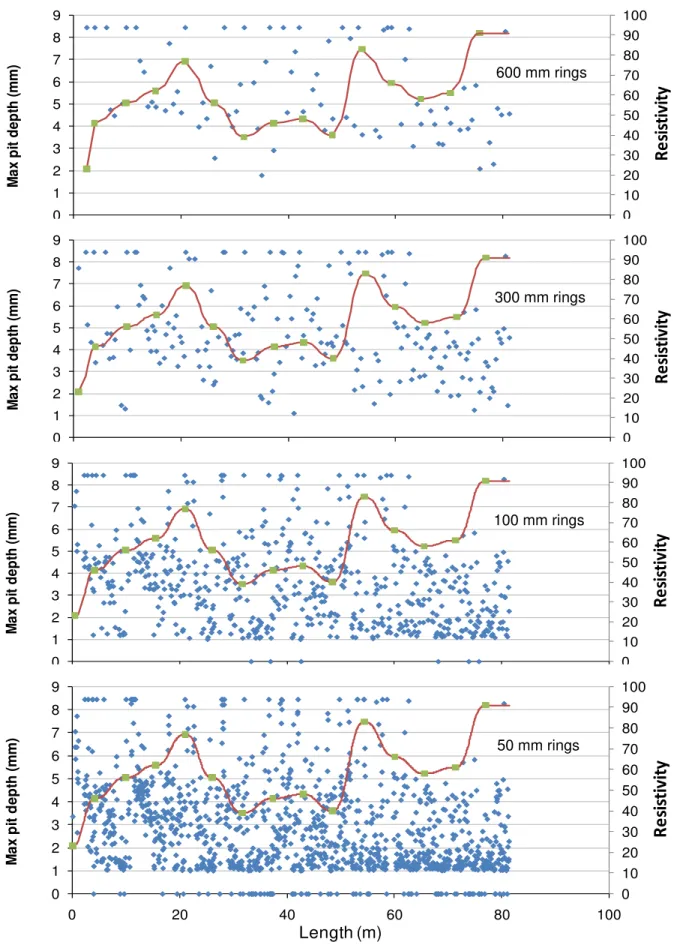
Figure 2 illustrates results obtained from Calgary data on pit-depth maxima. One thousand (1000) sampling simulations were run for each of the sampling schemes (e.g., 1000 simulations for 4 sites with 1 ring per site, 1000 simulations for 5 sites with 1 ring per site, and so on) and the histograms, means and standard deviations (SDs) were computed for the truncated Gumbel distribution parameters. A few observations can be made:

• Location parameter: The simulation mean value for the location parameter in all the sampling schemes is greater than that of the true population parameter, probably due to the long right tail (see example case). However, as expected, the simulation mean values tend to converge towards the true population value as the number of sites and the number of rings per site increase and the corresponding simulation SDs become smaller.

• Scale parameter: The simulation mean values for the scale parameter approximate well the true population parameter.

• As can be expected, the simulation SD values decrease as the number of sites increases.

• For a given number of sites n, the simulation SD decreases somewhat as k (the number of adjacent rings per site) increases. For a given number of total rings (e.g., 8 rings), the simulation SD is smaller for the.

(9)

1.989 1.564 0.0 0.5 1.0 1.5 2.0 2.5 0.0 0.5 1.0 1.5 2.0 2.5 5 tes 1 ng 6 sites 1 ring 7 sites 1 ring 8 sites 1 ring 9 sites 1 ring 10 sites 1 ring 4 sites 2 ring 5 sites 2 ring 6 sites 2 ring 7 sites 2 ring 8 sites 2 ring 9 sites 2 ring 10 sites 2 ring 4 sites 3 rings 5 sites 3 rings 6 sites 3 rings 7 sites 3 rings 8 sites 3 rings 9 sites 3 rings 10 sites 3 ring

St

a

n

d

a

rd

de

v

ia

ti

o

n

Mea

n

va

lu

e

s

Pit‐depth maxima 50 mm ring sampling (1000 simulations per case)

Scale mean Location mean Population location Population scale Scale StDev. Location StDev. 4 sites 1 ring si ri

Example case (1000) simulations

Population 0 Population 0.00 0.05 0.10 0.15 0.20 0 1 2 3 4 5 6 7 8 9 Histogram of parameters (pit maxima in 50 mm rings, 4 sites, 1 ring per site ) Scale Location

(10)

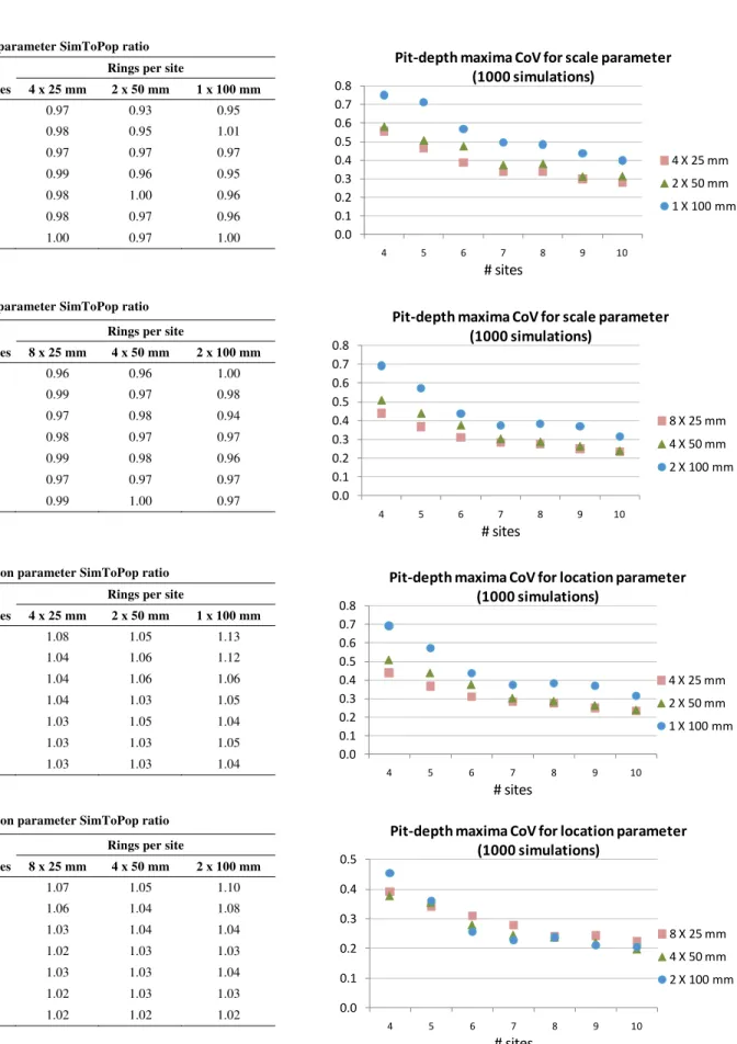
Scale parameter SimToPop ratio

Figure 3. Kansas City pit-depth maxima: comparisons of various sampling schemes.

Rings per site

# sites 4 x 25 mm 2 x 50 mm 1 x 100 mm 4 0.97 0.93 0.95 5 0.98 0.95 1.01 6 0.97 0.97 0.97 7 0.99 0.96 0.95 8 0.98 1.00 0.96 9 0.98 0.97 0.96 10 1.00 0.97 1.00

Scale parameter SimToPop ratio Rings per site

# sites 8 x 25 mm 4 x 50 mm 2 x 100 mm 4 0.96 0.96 1.00 5 0.99 0.97 0.98 6 0.97 0.98 0.94 7 0.98 0.97 0.97 8 0.99 0.98 0.96 9 0.97 0.97 0.97 10 0.99 1.00 0.97

Location parameter SimToPop ratio Rings per site

# sites 4 x 25 mm 2 x 50 mm 1 x 100 mm 4 1.08 1.05 1.13 5 1.04 1.06 1.12 6 1.04 1.06 1.06 7 1.04 1.03 1.05 8 1.03 1.05 1.04 9 1.03 1.03 1.05 10 1.03 1.03 1.04

Location parameter SimToPop ratio Rings per site

# sites 8 x 25 mm 4 x 50 mm 2 x 100 mm 4 1.07 1.05 1.10 5 1.06 1.04 1.08 6 1.03 1.04 1.04 7 1.02 1.03 1.03 8 1.03 1.03 1.04 9 1.02 1.03 1.03 10 1.02 1.02 1.02 0.0 0.1 0.2 0.3 0.4 0.5 0.6 0.7 0.8 4 5 6 7 8 9 10 # sites Pit‐depth maxima CoV for scale parameter (1000 simulations) 4 X 25 mm 2 X 50 mm 1 X 100 mm 0.0 0.1 0.2 0.3 0.4 0.5 0.6 0.7 0.8 4 5 6 7 8 9 10 # sites Pit‐depth maxima CoV for scale parameter (1000 simulations) 8 X 25 mm 4 X 50 mm 2 X 100 mm 0.0 0.1 0.2 0.3 0.4 0.5 0.6 0.7 0.8 4 5 6 7 8 9 10 # sites Pit‐depth maxima CoV for location parameter (1000 simulations) 4 X 25 mm 2 X 50 mm 1 X 100 mm 0.0 0.1 0.2 0.3 0.4 0.5 4 5 6 7 8 9 10 # sites Pit‐depth maxima CoV for location parameter (1000 simulations) 8 X 25 mm 4 X 50 mm 2 X 100 mm

(11)

• scheme in which k is smaller (e.g., 8 sites with 1 ring per site will have a smaller simulation SD than 4 sites with 2 rings per site). This is expected due to the fact that adjacent rings are not iid and that the population is better represented by more sites.

• The same general behavior described above was observed in the other cities data sets as well, including for 25 and 100 mm rings

A comparison of the performance of various ring-length samples has to be done on a relative basis. Two criteria of accuracy and precision were used to make this comparison. Accuracy was measured as the ratio between the simulation mean value for the parameter and the population parameter (referred to here as SimToPop ratio). Precision was measured as the ratio between the simulation parameter SD and the simulation parameter mean (this ratio is also known as the coefficient of variation or CoV). Figure 3 shows the results of these comparisons in terms of SimToPop ratio and CoV for pit-depth maxima in the Kansas City dataset. It should be noted that the total length of rings per site is equal in every comparison, i.e., 4 adjacent rings of 25 mm were compared to 2 adjacent rings of 50 mm and to 1 ring of 100 mm, or 8 adjacent rings of 25 mm were compared to 4 adjacent rings of 50 mm and to 2 rings of 100 mm. A few observations on these comparisons are noted:

• Scale parameter- accuracy (two top tables in Figure 3): accuracy obtained from the simulations for the scale parameter in the pit-depth maxima was quite high in all cases, as manifested by the SimToPop ratios, which were all quite close to unity. The 25 mm rings did slightly better but this was not significant. No significant improvement in the SimToPop ratio was noted as the number of sites increased

• Scale parameter- precision (two top charts in Figure 3): while the precision of the 25 mm and 50 mm rings schemes was comparable, the 100 mm ring scheme displayed relatively poorer precision (higher CoV). In all cases, the increase in the number of sites led to improvement in the precision of the scale parameter obtained from the simulations. For a given number of locations, precision improves if more adjacent rings are sampled (despite the fact that these adjacent rings are not iid).

• Location parameter accuracy (two bottom tables in Figure 3): accuracy obtained from the simulations for the location parameter in the pit-depth maxima was comparable (and quite high) in the 25 mm and 50 mm rings and somewhat inferior in the 100 mm rings, especially in the schemes with the fewer sites. All sampling schemes showed clear improvement when the number of sites increased.

• Location parameter- precision (two bottom charts in Figure 3): the precision of the 25 mm and 50 mm rings schemes was comparable in all sampling schemes, however the precision of the 100 mm rings was lower for the scheme involving one ring per site. In all cases, the increase in the number of sites led to improvement in the precision of the location parameter obtained from the simulations. For a given number of locations, precision improves if more adjacent rings are sampled (despite the fact that these adjacent rings are not iid).

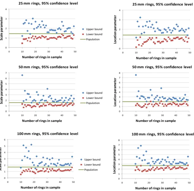
The likelihood ratio confidence bounds (LRB) is a commonly used method to find the confidence bounds of probability distribution parameters that are estimated based on a relatively small sample size (Kováčová, 2009; Reliasoft, 2008). This method was applied here as follows. We generated 39 random samples for ring lengths of 25, 50 and 100 mm to test how ring length influences the confidence bounds for distribution parameters. Using the notation defined earlier in this chapter, the samples comprised n*k rings where

n = 10, 11, 12, …, 49 (# of sites); and k = 1 (# of rings/site).

Figure 4 illustrates the comparisons of the results (scale and location parameters) for pit-depth maxima for the specific data set for Calgary. As is expected, it is clear that in general, the higher the number of rings in the sample the narrower the confidence interval. Additionally, it appears that the 95% confidence interval for the 25 mm ring population is narrower than for the longer rings, which may point towards a higher predictability of pit-depth maxima parameters in the shorter rings. This, however, is based on samples taken from a relatively small length of exhumed pipe and would require more extensive tests to validate.

(12)

0 1 2 3 4 0 10 20 30 40 50 Sca le pa ra m e te r Number of rings in sample 25 mm rings, 95% confidence level 0 1 2 3 4 0 10 20 30 40 50 Lo ca ti o n par a me te r Number of rings in sample 25 mm rings, 95% confidence level Upper bound Lower bound Population 0 1 2 3 4 5 6 7 0 10 20 30 40 50 Sc a le par a m e te r Number of rings in sample 50 mm rings, 95% confidence level 0 1 2 3 4 5 6 7 8 0 10 20 30 40 50 Lo ca ti o n pa ra m e te r Number of rings in sample 50 mm rings, 95% confidence level Upper bound Lower bound Population 0 1 2 3 4 5 6 0 10 20 30 40 50 Sca le pa ra m e te r Number of rings in sample 100 mm rings, 95% confidence level 0 1 2 3 4 5 6 7 8 0 10 20 30 40 50 Lo ca ti o n pa ra m e te r Number of rings in sample 100 mm rings, 95% confidence level Upper bound Lower bound Population

Figure 4. Calgary pit-depth maxima: parameter confidence bounds for various ring lengths

4. INFERENCE ABOUT DI PIPE CONDITION

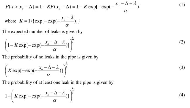
Two classes of inferences can be constructed based on the statistical properties of corrosion pit geometries identified in this research. The first class addresses the presence of corrosion through-holes causing leaks and the second addresses the remaining structural resiliency of the pipe. Since the predominant failure mode in DI pipes is corrosion, we focus here on the former, i.e., presence of corrosion through-holes causing leaks. For this we use the concept of return period. Return period (or recurrence interval) usually refers to the estimated time between subsequent occurrences on of an event (e.g., earthquake, intense storm, etc.). The principles for the computation of recurrence of events in time can also be used to compute recurrence of events in space, e.g., the recurrence of a corrosion hole in a given length of pipe.

Let a pipe of length L and wall thickness xo be divided into a population of rings of length l, and let the

(13)

pipe is defined as a situation where the remaining wall thickness is smaller than ∆ mm. The probability of a leak in any ring is

)] exp( exp[ 1 ) ( 1 ) (

λ

=

∑

α

λ

−

χ

∑

= = ) ) (5) where )] ) ( exp( exp[ )] ) ( exp( ) ( exp[ ) , (

α

λ

α

λ

α

λ

α

Z x Z x Z x f o i i − − − ⋅ − − − − − =

Figure 5 illustrates the expected number of leaks and their 95% confidence bounds computed for various ring length and various size samples, using the Calgary data set. It is important to note that the population for the number of leaks represented by the horizontal line in Figure 5 is the theoretical (computed) expected number of leaks based on the parameters of the respective ring populations, i.e., 25, 50 and 100 mm ring populations. It is not the actual number of perforations detected through scanning of the pipe. The reason for this requires a somewhat detailed explanation. The right-truncated Gumbel probability distribution was found to fit well the histogram of pit-depth maxima in all the data sets. However, the fitting exercise was carried out with the actual perforated rings excluded from the analyzed data. This is because the perforated state is a so-called “absorbing state”, meaning that the count of perforated rings continually grows over time until (given enough time) all rings will perforate. Consequently it is not possible to fit a conventional probability distribution in the data in which the frequency of at upper bound is continually growing. Consequently, the methods proposed here are suitable to estimate the number of expected leaks in a pipe that is not overly deteriorated and has not already experienced several leaks. The three data sets for this study came from rather deteriorated pipes (Calgary experienced 28 perforations (through-holes) in the 50

(14)

Figure 5. Calgary data: confidence bounds for the expected number of leaks for various ring lengths. mm ring population and Kansas City and Louisville experienced 12 and 20 perforations, respectively) and therefore the number of actual perforations could not be accurately estimated with this method. It is possible that this method could be modified or an alternative method found to suit deteriorated pipes as well, but this requires further research.

Based on Figure 5 (as well as on similar tests implemented on the other data sets), it is clear (as expected) that confidence bounds become narrower as the number of rings in the sample increases, but it cannot be said with any certainty which ring length (25, 50 or 100 mm) is preferable. This too needs to be further investigated in future research.

5. CONCLUDING COMMENTS

Considering that the sampling scheme and corresponding inferences were based on a few exhumed pipes, it is difficult to draw definitive conclusions and make definite recommendations without investigating more pipes from geographically diverse locations. As a preliminary conclusion to assess ductile iron pipe condition, it appears preferable to sample shorter rings (10 - 50 mm) and take minimum of 7 to 10 samples (sites, in 100 m long pipe). This may appear as a costly endeavor for a 100 m pipe but it is likely that the number of required samples to assess a longer pipe will not increase substantially.

While the modeling part of any research is an important foundation, upon which all processes are created, the sampling and inference parts are the anchors that tie this research to reality. Some insight into the sampling and inference issues was provided but more research is required to possibly transform this entire approach into a viable non-destructive, non-intrusive pipe evaluation technique. A cost benefit analysis of precision versus sampling cost is needed, where accuracy and precision are considered in conjunction with costs corresponding to false positives and false negatives, to arrive at a cost-efficient sampling scheme. Further, a modification or alternative model to accommodate highly deteriorated pipes would be beneficial. Finally, the extension of the condition inference model to cast iron pipes, where the predominant failure

0 1 2 3 4 5 6 7 8 9 0 10 20 30 40 50 ct le a Number of rings in sample 25 mm rings, 95% confidence level Ex pe e d # k s Upper bound Lower bound Population 0 1 2 3 4 5 6 7 8 9 10 11 12 13 0 10 20 30 40 50 Number of rings in sample 50 mm rings, 95% confidence level 0 1 2 3 4 5 6 7 0 10 20 30 40 50 Number of rings in sample 100 mm rings, 95% confidence level

(15)

mode is structural, will require the development of a statistical inference mechanism about the remaining structural integrity of the pipe.

ACKNOWLEDGEMENT

This research project was co-sponsored by the Water Research Foundation (WRF – formerly known as the American water Works Association Research Foundation – AwwaRF) and the NRC with in-kind

contributions from water utilities in the United States and Canada.

.References

Kleiner, Y., B. Rajani and D. Krys. (2010). “Impact of soil properties on pipe corrosion: re-examination of traditional conventions”, Proceedings Water Distribution System Analysis 2010 - WDSA2010, Tucson, AZ, Sep.

Kováčová, M. (2009). “Reliability likelihood ratio confidence bounds”. Aplimat – Journal of Applied Mathematics, 2(2): 217-225.