Broadband nanosensing using heterodyne interferometry

(1)

Broadband Nanosensing using Heterodyne

Interferometry

by

Bennett Landman

MASSACHUSETS MNTITUT M _{OF TECHNOLOGY} T T

JUL 3

1 2002

LIBRARIES

Submitted to the Department of Electrical Engineering and

Computer Science

in partial fulfillment of the requirements for the degree of

Master of Engineering in Electrical Engineering and Computer Science

at the

MASSACHUSETTS INSTITUTE OF TECHNOLOGY

February 2002

@

Bennett Landman, MMII. All rights reserved.

The author hereby grants to MIT permission to reproduce and

distribute publicly paper and electronic copies of this thesis document

in whole or in part.

/'

Author ...

Department offlectrical Engineering and

Computer Science

January 9, 2002

Certified by..

_V

Accepted by....

Dennis Freeman

, Associate Professor

yThesgSupervisor

Arthur C. Smith

Chairman, Department Committee on Graduate Theses

(2)

(3)

Broadband Nanosensing using Heterodyne Interferometry by

Bennett Landman

Submitted to the Department of Electrical Engineering and Computer Science

on January 9, 2002, in partial fulfillment of the requirements for the degree of

Master of Engineering in Electrical Engineering and Computer Science

Abstract

Interferometric and bright field microscopy methods for measuring vibrational, peri-odic motions have been well established. We extend existing measurement techniques to encompass detection of broadband, aperiodic motions of microscopic beads along one dimension. In the device, a coherent 488 nm laser beam is split into two beams with a relative frequency shift of 3.4 MHz. The beams are overlapped on a target slide to form a rolling interference pattern. A latex bead is placed in the pattern, and a photomultiplier incoherently collects the scattered light. The amount of light scat-tered by the bead varies sinusoidally due to the rolling interference pattern. Motions of the bead modulate the phase of the sinusoid. The detected signal is sampled at 10 megasamples/second and digitally phase demodulated. Over a frequency bandwidth of 10 kHz to 1 MHz, a broadband rms noise density of 19 pm/VHz was observed for a

1.5 pm diameter bead. Due to sub-500 Hz equipment vibration, the mean rms noise

level was 101 pm//Hz over DC to 100 kHz. The system would allow measurements as small as 30 nm for an observation bandwidth of 2.5 MHz. Further enhancements to increase the power of collected light could extended the resolution to characterize the Brownian motion of beads in the tectorial membrane.

Thesis Supervisor: Dennis Freeman Title: Associate Professor

(4)

(5)

Acknowledgments

First, I would like to thank my advisor, Dennis Freeman, for his inspiration, confidence and persistent support. He has helped solve the most perplexing problems. His enthusiasm permeates the eighth floor and has helped make this a wonderful (yet sleepless) experience. I greatly appreciate the advice of Charles Sodini and Howard Schrobe, who guided my thesis aspirations and introduced me to Professor Freeman.

My fellow eighth floor students have provided invaluable assistance over the past

year. With extreme patience, Stan Hong has taken countless hours away from his research to explain a myriad of ideas and has proofread this work with insightful comments. A.J. Aranyosi has been the utmost authority on how to get things done in lab. Thank you for putting up with nearly continuous questions. Andy Copeland and Salil Desai loaned me key components from their work at the last minute (sometimes before they knew that they had). Janice Balzar, the lab secretary, always came through despite my unconscious attempts to thwart her. Thanks to Amy Englehart for being here during those lonely morning hours. From U.C. Berkeley, Jen Nickel and Temina Madon have been extremely helpful editing this document.

MIT would not have been what it was without friends whose support has preserved most of the sanity in this crazy life we have lived. I thank all of those people who I have been fortunate enough to call my friends.

Thanks to Mom and Dad (Petra and Gary Landman) for always supporting me in everything that I do. Mom, the care packages and phone calls have meant more to me than I could ever tell you. Dad, I keep your writing advice close at hand - see you can teach a computer nerd something. Rebeccah, you are the world's best sister. Zach, thanks for making me the most popular big brother in high school.

To close, I would like to thank my wife, Melissa Ohsfeldt Landman. She has put up with more than I can imagine during this extended crunch period and has encouraged me to focus my thoughts so I could rejoin her as quickly as possible.

(6)

(7)

List of Figures

1-1 Conceptual schematic. . . . . 2-1 2-2 2-3 2-4 2-5 2-6 2-7 2-8 17

Two-dimensional model of a sphere in a fringe pattern. . Fringe formation. . . . . Fringe period with beam separation. . . . .

Illustration of fringe distortion. . . . . Model of scattering off a sphere. . . . . Examples of scattering profiles. . . . . Relation of fringe spacing to scattering intensity. . . . . . The detection process. . . . .

. . 22 24 . . 25 26 . . 28 29 31 36 3-1 Lever model of the inner ear .. . . . .

3-2 Approximate range of bead movement at room temperature. . . . . .

3-3 Ratio of scattering cross-section to geometric cross section. . . . .

3-4 Modeled collected fraction of scattered light. . . . .

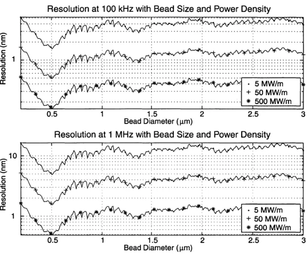
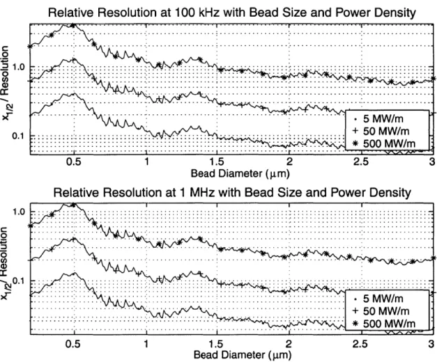
3-5 Modeled sensitivity of detection system in nanometers with latex spheres in 488 nm light. . . . .

3-6 Modeled sensitivity of detection system relative to the modeled motion

of a latex sphere undergoing Brownian motion with 488 nm illumination. 4-1

4-2 4-3 4-4

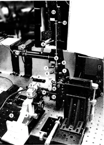
Stationary fringe projector optics layout. . . . . Microscope construction. . . . . Signal processing method. . . . . Circuit design for piezo position buffer. . . . .

42 46 48 49 51 53 56 57 58 60

(12)

4-5 Least squares fit to photomultiplier gain. . . . . 4-6 Photomultiplier field of view relative to camera. . . 4-7 Detection system noise floor. . . . . 4-8 In-line piezo sensor analysis. . . . . 4-9 Out-of-line coupling. . . . . 4-10 Demonstration of modulation. . . . . 4-11 Measured data for a 0.5 pm bead experiment. . . .

4-12 Measured modulation visibility. . . . . 4-13 Detected power with bead size. . . . . 4-14 Scattering signal with position for a 0.5 pm bead. 4-15 Power spectral density of a stationary 1 pm bead. 4-16 Noise power with detected power with a 5 MHz band

5-1 5-2 5-3 5-4 5-5 5-6 . . . . 62 . . . . 63 . . . . 64 . . . . 65 . . . . 66 . . . . 69 . . . . 70 . . . . 71 . . . . 71 . . . . 72 . . . . 73 width . . . . . . 74

Heterodyne fringe prototype optics. . . . . . Target stage with feedback stabilized piezo. Target stage with open-loop piezo. . . . . . Heterodyne prototype signal processing. Acousto-optic modulator drive signal... Demodulated motion data. . . . . . . . . 78 . . . . 79 . . . . 80 . . . . 8 1 . . . . 83 . . . . 88 5-7 Laser Doppler measurement of relative motion between piezo stage and

fringe projecting objective. . . . .

5-8 RMS noise with bead size for DC to 100 kHz. . . . . 5-9 Median white noise level for broadband noise above 500 Hz... 5-10 Observed modulation visibility. . . . . 5-11 Open-loop piezo response to a 5 kHz sine wave. . . . .

5-12 Power spectral density estimate of noise in an open loop system. . . .

5-13 Power spectral density of light detected during a 300 Hz square wave

stim ulus. . . . . 5-14 Power spectral density estimate of the motion stimulated by a 300 Hz

square w ave. . . . . 90 91 92 92 93 94 95 95

(13)

(14)

(15)

Chapter 1 Introduction

1.1 Motivation

Engineering systems are getting smaller and harder to see. New microfabrication tech-niques are narrowing the boundaries between molecules and machines. Accelerome-ters that are smaller than the diameter of a human hair are now commonplace.

To understand the mechanics of these new machines, we require technologies that can measure minute motions without interfering with operation. Light microscopy is a powerful, minimally invasive tool, but diffraction effects limit the achievable resolution to half the wavelength of the light[1].1 A method of using light microscopy to achieve

nanometer resolution with image processing techniques has been demonstrated[2]. This method requires that motion be periodic and that stroboscopic illumination be used to freeze motion. This method cannot be used to detect nanometer motions over a broad frequency range.

An alternative approach to achieving high resolution motion measurements has been to use optical interference to generate fringes that facilitate higher contrast detection[3]. Laser interferometry encompasses a class of methods that have proven extremely effective for determining displacement, flow velocity, and vibrational mo-tion. Within the general class of methods, there are two distinct signal detection

(16)

els: heterodyne and direct detection. Heterodyne detection interferometric methods interfere a probing beam with a reference beam[4]. The probing beam and reference beams are at slightly different frequencies, so their interference pattern "optically beats." The motion of the bead introduces a phase shift into the beating signal. In direct detection interferometry, beams are overlapped to form fringe patterns on a target[4]. The position of the target within the fringe pattern determines the intensity of light scattered. The light is incoherently collected by a detector.

This research develops an interferometric system that expands on existing vibra-tion measurement technologies to encompass broadband nanosensing. Previous sys-tems were developed to measure periodic ranges of movement at a specific frequency[5,

6]. As such, they may be categorized as narrow-band methods. This research focuses

on the ability to detect aperiodic motions over a broad range of frequencies. Inter-ferometric illumination is used to create an "optical radio" that can detect aperiodic, broadband motions as shown in Figure 1-1.

1.2 Narrow-Band Interferometric Techniques

In 1964, Yeh and Cummins observed that the frequency of light changed as it passed though a stream of moving particles[7]. The interaction of the moving particles with the light introduced a Doppler shift in the scattered light. By carefully measuring the amount of frequency shift, they were able to determine stream velocity. Steady advances and refinements of their technique have lead to a variety of direct and het-erodyne methods that are collectively known as laser Doppler methods[3]. These methods routinely achieve 20 pm spatial accuracy with microsecond temporal resolu-tion. A key advantage of using interferometric methods over physical contact methods is that the particle flow is not disturbed during observation. However, the methods are not without drawbacks; the particle stream must be optically transparent and additional doping may be necessary to increase the density of scattering particles.

In 1980, Buunen demonstrated a heterodyne laser Doppler velocity meter to mea-sure vibrational motions of a cat tympanic membrane[5]. One beam was used to

(17)

Structured

Illumination

Motion

Scattered

Detected

Light

Signal

Figure 1-1: Conceptual schematic. The device is essentially an "optical radio." Struc-tured illumination, lasers, overlap to form a rolling interference pattern. In the region of overlap, indicated by the gradient, the brightness varies sinusoidally with time and position. A target, represented by the white dot, is placed in the rolling fringe pattern. If the target is stationary, the scattered light intensity oscillates sinusoidally. Target movement along the axis of fringe variation introduces a phase shift in the oscilla-tions of the scattered light. The light is collected by a photomultiplier, represented

by a rectangle with an oval aperture. The photomultiplier current is band-limited

and digitized. A computer utilizes phase demodulation algorithms to determine the motion of the target in the fringe pattern.

(18)

illuminate a 100 pm spot on the membrane while researchers stimulated the mem-brane with acoustic waves. Memmem-brane motion generated a Doppler shift in the light scattered from its surface. Scattered light was interfered with a reference beam on a detector. The reference beam was frequency shifted by 400 kHz, so the Doppler

shifted signal was modulated at 400 kHz. The detected signal was electronically

en-hanced by filtering, averaging, and time sensitive detection. The Buunen detection method was able to measure vibrations on the order of 0.1 nm.2 _{Their maximum} observable frequency was 2.24 kHz.

In 1987, van Netten presented a direct detection laser interferometry microscope for use on fish lateral line organs[6]. He illuminated a 1.15 pm diameter polymer bead with a fringe pattern. The heterodyne frequency of the fringe pattern was 400 kHz and the fringe spacing was approximately 0.7 pm. This device detected vibrational displacements from 0.3 nm to 300 nm with observable motion frequencies of 10 to

500 Hz. A glass sphere mounted on a piezoelectric device was used to stimulate

vibrations.

1.3 Broadband Laser Interferometry

When particle motion cannot be assumed to be periodic, the methods developed by Buunen and van Netten to generate interference patterns and detect scattered light can still be used[5, 6]. However, different signal processing methods are required. Furthermore, temporal correlation cannot always be exploited to reduce noise. This research develops a technique for measuring motion that can be tuned to exchange observation bandwidth for spatial resolution. The fundamental benefit from this method is that the interferometer can be adjusted to suit a range of applications.

One such application of the broadband laser interferometer is in the study of hear-ing. Research has shown that humans can detect sound vibrations with amplitudes as small as 1 pm[5]. The tectorial membrane, a thin gelatinous structure in the ear, has been shown to play a key role in producing the vibrations that are detected by

2

(19)

the sensory hair cells. Vibration sensing interferometers have been used to determine the frequency responses of the structure, but some material properties, such as the stiffness of the gel, remain elusive.

One method of measuring stiffness is to apply a force and measure displacement. If the material behaves as an elastic spring, then displacement will be linear with force. If the material behaves as a viscous fluid, then force will be proportional to ve-locity. A gel, such as the tectorial membrane, has both viscous and elastic properties. Mechanical properties of gels which are determined by the gel's cross-linked network of polymeric macromolecules, are nonlinear. We therefore seek methods to measure mechanical properties of the tectorial membrane for small forces and small displace-ment. The ultimate limiting range of detectable movement would be determined by the Brownian of the system. Using the force-displacement method, displacements of the tectorial membrane as small as hundreds of nm have been measured in response to forces as small as tens of nN[8]. However these forces and displacements are orders of magnitude greater than those that occur in hearing.

An alternative approach for measuring the visco-elastic behavior in a gel is to let thermal energy drive Brownian motion. The material properties may be calculated from the statistics of gel motion given the random thermal energy. Narrow-band mea-suring systems could not be used in this experiment because the motion is not driven at a particular frequency. Furthermore, the range of Brownian motion drastically decreases with increasing target size, so localized measurements of motion are neces-sary. A broadband laser interferometer similar to this research design would enable the measurement of visco-elastic properties through statistical analysis of Brownian motion.

(20)

(21)

Chapter 2 Survey of Technology

The primary components of the interferometer design are a fringe projector, a scat-tering target, and a detection system. The fringe projector overlaps two coherent beams of similar wavelengths in a volume of space. The beams constructively and destructively interfere to form a three dimensional volume of bright and dark fringes.

A target, such as a small bead, is placed in the illuminated area and interacts with

and scatters light. The measured scattering intensity depends on the bead position and angle of observation. A detection system collects the scattered light and infers the target position.

As Figure 2-1 illustrates, bead and fringe movements in the out-of-plane directions will not change the illumination of the bead since the fringe pattern varies along only one axis. Changes in the intensity of the scattered light are caused by movements of the particle or the fringe pattern. Therefore, a two beam fringe projection system is limited to measuring motions in one dimension.1

The intensity of scattered light is proportional to the incident light on the sphere during the measurement interval. For example, the light is at a minimum when the bead is mostly covered by dark fringe bands and at a maximum when it is covered

by light fringe bands. If the fringe pattern and sphere are assumed to be stationary

'Multidimensional measurement systems are possible with systems of more than two beams. This research focuses solely on the case of two stationary beams. A discussion of multi-beam possibilities is presented in the closing remarks.

(22)

s

a

9

I

-4|

x(t)

I(--Figure 2-1: Two-dimensional model of a sphere in a fringe pattern. A sphere is represented by a disc of a diameter, a. The axis of fringe variation is represented by x. The distance between consecutive fringe minima is the fringe period, s. Sphere position is distance from the center of the sphere to a fixed point in space that is arbitrarily set to the initial location of the nearest band of median fringe intensity. Each ^-^ plane represents a plane of constant fringe intensity. Each point on the surface of the sphere is illuminated by the intensity of the fringe pattern at that point. The range in intensity of scattered light was estimated using the two-dimensional model (the disc model), but a three-dimensional model was used to calculate the actual scattering functions.

(23)

over the measurement period, then the scattered light will vary with the position of the sphere relative to the fringes. Thus, the motion of the sphere may be determined from the scattered light[3].

2.1 Fringe Projection

2.1.1 Interference

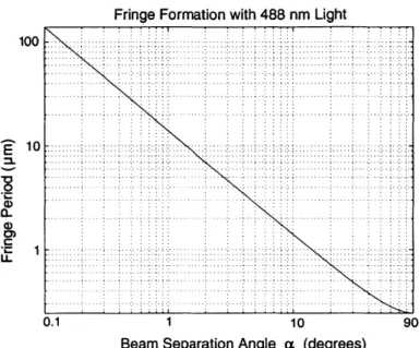
Techniques for generating well-defined fringes have been commonly used in laser interferometry[3]. Fringe patterns are generated by interfering coherent light beams of similar frequencies. Bright areas are formed in the region where the electric fields constructively interfere and dark areas are formed where they destructively interfere. If the beam wave fronts are sufficiently planar and the optical frequencies well-defined, lines of alternating brightness will form at an angle bisecting the angle of intersection (Figure 2-2). The fringe spacing depends on the plane of observation and is given by

s =

A

(2.1)

2n sin a cos q

where A is the optical wavelength, n is the index of refraction of the medium, a is the half angle of beam separation, and

#

is the angle of rotation between the plane containing the beams and the plane containing the bisector of the beams and the axis of fringe variation. This relation is plotted in Figure 2-3. When the beams are of exactly the same frequency, the pattern is a standing wave and the envelope is stationary in time. If the beams are of different frequencies, then the bright and dark bands roll at the rate of frequency separation.

Figure 2-4 illustrates effects of non-planar wave fronts on fringe formation. In order to achieve planar wave fronts, beams are typically overlapped at their waists. The fringes will be significantly distorted if misalignment in optics causes the beams to overlap where the wave fronts differ from planar. Spherical aberration in the optics causes divergence in the beams that leads to non-uniform fringes. Furthermore, if the path lengths of the beams differ by more than the light source coherence length, the

(24)

91

X

Figure 2-2: Fringe formation. When two coherent beams of sufficiently similar fre-quencies (11 and 12) overlap, they form fringes. The figure shows a reference frame

relative to the fringes with the x - y plane as the plane of observation and fringe

intensity varying only along ^. The half beam separation angle, a, is half of the angle between the beams in the plane containing the two beams (dark gray shading). The rotation angle, q, is the angle of rotation between the plane containing the beams (dark gray shading) and the plane that contains the bisector of the beams (dotted centerline) and the x-axis (X) (plane indicated by light gray shading).

(25)

Fringe Formation with 488 nm Light ... ... ............. ... .......... ..... ..... ........... ..... .. ........ .......... ......... .... ....... . ......... ... _.._._....._..._{. .}.... _...._..._..... _._._...._..... _..._. _...._.._...._.._.._.... ...... .... . ........ : ............ ......... ........... .. ........ ..... . ... ........... .... ............ ........ .... ..... ......... ............. .. ........ ..... ....... . ............ ....... ..... ......_... ... ...................... ....... .. ........ ...................... .. .............. .......... ...... .......... ... ........ .. ........ ...... 1 10

Beam Separation Angle a (degrees)

Figure 2-3: Fringe period with beam separation. The relation between fringe period and beam separation is shown for an index of refraction of 1 and rotation angle of 0 degrees.

beams will not fully interfere and the contrast between the light and dark fringes will decrease[3].

2.1.2 Beam Waist Formation

The waist of a beam occurs very close to the location where the beam is in focus. The diffraction limited diameter at the waist is approximately

4Af

7rD (2.2)

where A is the wavelength of light,

f

is the focal length used to focus the beam, and

D is the diameter of the collimated beam before it was focused[6].

100 10 C LL 0.1 90 1

(26)

(a) Ideal fringes.

(b) Fringes from divergent beams.

(c) Fringes from non-planar beams.

Figure 2-4: Illustration of fringe distortion. When two planar beams of the same frequency overlap, the wave fronts interfere to form straight fringes (a). Straight, non-parallel fringes are formed if the overlapping beams are divergent as in (b). If the beam wave fronts are not planar, then fringe patterns may be curved as well as skew (c).

(27)

2.2 Optical Scattering

2.2.1 Mie Scattering

Determining the optical scattering properties of a particle involves calculating the potential function at all points in space due to interaction of the particle with an incident wave. The use of a spherical target greatly simplifies the problem since Mie developed an exact analytical solution for a single beam scattering off of a sphere[9]. The amount of scattered light has been found to depend on the ratio of the index of refraction of the sphere to that of the medium and a sizing parameter given by

27ra

X = (2.3)

where a is the diameter of the target sphere. In general, scattering intensity is a function of scattering angle, orientation angle, and polarization of incident radiation (Figure 2-5). Symmetry constraints for scattering off a sphere dictate that the abso-lute polarization and orientation angles are not relevant. Rather, the polarization as observed in a scattering plane and the scattering angle are sufficient.

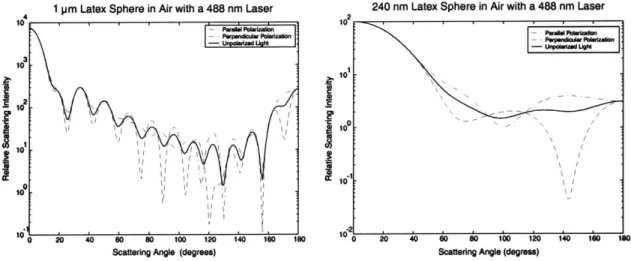
The scattering of more complicated waves may be treated as a superposition of component waves. The scattering function of unpolarized light may be found by averaging the scattering functions for both parallel and perpendicular polarized light. Figure 2-6 illustrates two different scattering functions that were computed with code adapted from Barnett's "Mie Scattering Toolbox" [10].

For small spheres, the greatest scattering intensity is generally in the same direc-tion as the incident light which is represented as higher intensity at the low angles in Figure 2-6. Unfortunately, there is also a large amount of unscattered light at low angles that makes separating the scattering signal from the illumination difficult. Scattering intensities typically decrease with increasing angle in a ripple-like manner, yet increase to local maximum near back scattering angles (180 degrees). The range of scattering intensity increases with the particle sizing parameter (Equation 2.3). Large particle scattering functions tend to vary more with angle than those of smaller ones.

(28)

x

Figure 2-5: Model of scattering off a sphere. Radiation is incident perpendicular to the ^ -

Y

plane in the positive Z direction as indicated by the series of arrows at the base of the figure. Light is scattered in all directions. One particular ray is indicated

by the dark arrow. The scattering angle,

#,

is the angle between ^ and the ray.

The orientation angle, 0, is relative to the coordinate system. The scattering plane (indicated with shading) is the plane defined by the ray and ^ axis.

(29)

1 pim Latex Sphere in Air with a 488 nm Laser

10 2

240 nm Latex Sphere in Air with a 488 nm Laser

3 10 -0

0 t10

10 'II0I ,

0 20 40 60 1 10 120 140 160 10 0 20 40 0 so tooA- 120 14o IGO ISO

Scattering Angle (degrees) Scattedng Angie (degrems)

Figure 2-6: Examples of scattering profiles. The left figure shows the scattering intensity of a 1 /Lm diameter latex particle in air when illuminated with 488 nm light. The size parameter is approximately 12.9 and the index of refraction is 1.59. The right figure shows the scattering intensity of a 240 nm latex sphere in water when illuminated with 488 nm light. The size parameter is approximately 3. The values of the scattering functions represent the relative amount of power scattered per angle when compared the angles from the same target.

The absolute magnitudes of the angular scattering calculations are only meaning-ful when compared to other angles for the same target. To find the absolute amount of power scattered, the scattering cross-section must be computed. The scattering cross-section is the area of the incident beam that contains an amount of light equal to that which is scattered by the sphere. With the relative proportion of scattering per angle and the total amount of energy scattered, the amount of energy scattered per angle can be computed. When using a lens to observe scattering, only a conical section of light may collected. The scattering function may be integrated to compute the total amount of light that can be collected with a lens.

2.2.2 Modulation Effects

In general, scattered light from a bead in a rolling fringe pattern is a combination of fixed intensity signal (the DC component) and an oscillatory signal (the AC compo-nent). As a bead moves in a fringe pattern, the intensity of scattered light changes

(30)

with position. Since light intensity is never negative and a target will never be com-pletely covered in an absolutely dark or bright band, the scattered light will have a

DC offset. The ratio of the peak-to-peak values of the AC signal to twice the DC

offset is defined as the modulation visibility. [3] It is a measure of the amount of signal power that the scattering signal carries. The modulation visibility is estimated from the disc model (Figure 2-1) by averaging the integral of a fringe pattern over a the cross-sectional area of a target. It is found to be

V=

1 2J1(7ra/s)1 (2.4)

ira/s

where J1 is a first order Bessel function of the first kind.

While the intensity of the reflected light is determined by the illumination and the properties of the sphere, the motion signal strength in the light signal depends also on the size of the sphere and spacing of the fringe pattern. If the fringe period is very small compared to the sphere diameter, then many fringes will overlap the sphere and the scattering intensity will only vary slightly with sphere movement because only a small fraction of the illumination will change. If the fringe period is large compared to the sphere, then larger sphere movements are required to generate detectable changes

in the scattering intensity[3] (Figure 2-7).

For a given sphere and cone of observation, the measured intensity of scattered light will be proportional to the total incident light on the sphere. The scattering signal may be characterized by the relationship between the sphere cross-section and illumination pattern. Without loss of generality, the position of the sphere in a sta-tionary fringe pattern is measured from a reference position that is half way between the initially nearest light and dark fringes. The sin function is periodic with 2wr, so any offset in x(t) of a integer multiple of s will not change the scattering intensity. Thus, bead motion, x(t) may referenced from an arbitrary period as long as the po-sition within the period is fixed. For simplicity, we selected the reference popo-sition as the nearest median level of fringe intensity at the initial time. In this context, the

(31)

HS

a

posi01ton

(a) Light modulation by movements of small fringes (a = 4s)

C

CD

a:

position

(b) Light modulation by movements of large fringes (a = s/3)

Figure 2-7: Relation of fringe spacing to scattering intensity. When the fringe pattern is small compared to the sphere, the modulation visibility is small (a). The peak to peak range of the AC signal is small compared to the DC offset. Since many fringes overlap the sphere, movements across fringes introduce relatively little modulation. When the fringe pattern is relatively large, the amount of reflected light changes slowly with movement (b). If the motions are constrained to a narrow range of movement, the modulation index will also be small.

0

S

0c Sphere Position Sphere Position a

(32)

scattering intensity is given by

I(t) = Io[l + V sin (27rx(t)/s)] (2.5)

where Io is the detected signal power from the reference position, V is the modulation visibility, x(t) is the particle position, and s is the period between two consecutive fringe maxima[6].

Notice that the relation between position x(t) and intensity I(t) in Equation 2.5 is nonlinear. One way to characterize the amount of information available in I(t) about

x(t) is to compute the modulation index. The modulation index is the maximum

amount of phase change due to motion. From Equation 2.5, the modulation index is max jx(t) - x(O)I(

A(D = 27r .(2.6)

S

When the fringes are stationary, the variation in scattering intensity changes with the particle's initial position. Since the sinusoidal illumination pattern changes more slowly near extrema than between extrema, particle movement near an extrema will cause less variation than if it were farther away from an extrema.

Quantitatively, the percentage fluctuation in scattering intensity due to motion, 7, for a given modulation index and initial position is defined as the difference between the maximum and minimum scattering intensity divided by the scattering intensity at the initial position. To demonstrate the effects of initial position, we consider a range of motion such that the scattering intensity is monotonic with position. For these modulation indices,

[1 + V sin (27rxo/s + Af)] - [1 + V sin (27rxo/s - A ] (27)

1 + V sin (27rxo/s)

2V Isin (A() cos (27rxo/s) _(2.8)

1 + V sin (27rxo/s)

where 7DC is the maximum percentage intensity fluctuation with a stationary fringe pattern and x0 is the initial sphere position. Since the range of intensity fluctuation

(33)

depends on the relative positions of the sphere and fringes, the ability to determine sphere position will also depend on the initial positions. Intuitively, this is undesirable because controlled placement of the sphere is extremely difficult. Furthermore, the frequency spectrum of the signal would overlap the spectra of common, low frequency noise sources such as changes in background illumination and secondary scattered light. The signal and noise would be hard to disambiguate because their frequency spectra would be similar.

One way to combat these problems is to roll the fringe pattern at a uniform velocity. We generalize Equation 2.5 to include a phase change due to rolling fringe motion, and the resulting scattering intensity is the motion signal phase modulated onto a carrier wave at the frequency of fringe oscillation,

1(t) = lo[1 + V sin (27rft + 27rx(t)/s)] (2.9)

where

f,

is the frequency of fringe oscillation as well as the carrier frequency of the motion signal[6]. The time average of the percentage fluctuation in scattering intensity becomes

I

[1 + V sin (27rft + 27rxo/s + AD)] - [1 + V sin (27rft + 27rxo/s - A(D)] I

7FM _{I + V sin (27wfct}

₊

_27rxo/s)

(2.10) Observe that the right hand side is periodic with period

fg',

so the time average may be computed with one period. An analytic solution may obtained by applying two change of variable operations, u = 27rft + 2-rxo/s and p = 1+ V sin (u), and utilizing the physical constraint that the visibility, V, is in the range of 0 to 1. Applying trigonometric substitution and integrating yields,

_2r1 I[1 + Vsin (U + A4D)] - [1 + Vsin (u -

AD)]|

7FM =du (211)

27r Iu=o 1 + V sin (u)

_ sin (AI)I 2r 2VIcos du (2.12)

21r =o 1 + V sin (u)

sin (AD)| w/2 1 1p + 21r

[ - - -dp

]

3 dp] (2.13)

(34)

2=sin(Ad)) _In _.+V

(2.14)

7r 1-V

The motion of the illumination pattern decouples the time average scattering intensity fluctuation from the initial position. Equation 2.14 shows that the mean percentage fluctuation given visibility is the average of the percentage fluctuation given the same visibility over all initial positions. Under these conditions, position may be determined with no dependence on absolute fringe position. Furthermore, since the signal is modulated up to a higher frequency, a high pass filter may be used to remove low frequency noise without affecting signal content.

Modulating the motion signal by a fringe movement does not lose information content as long as aliasing does not occur. Each frequency component of the motion signal, x(t), produces a series of side-bands around the carrier frequency in the Fourier transform of I(t). These side-bands rapidly decrease outside

AFsideband = A fsideband (2.15)

where fsideband is a specific frequency component of the motion signal. Low motion frequencies are represented by compact side-bands around the carrier while high fre-quencies are more spread out[11]. Thus, if the motion signal may be assumed to be frequency limited to fmax, the carrier frequency must be significantly greater than A'Dfmax to avoid aliasing.

2.2.3 Effective Modulation Index

When investigating the performance characteristics of the system, the change in op-tical power scattered from two different positions of interest is an important consid-eration. If the change is small, then only a small amount of noise can be tolerated while maintaining the ability to distinguish between the two positions. Conversely, a larger amount of noise can be tolerated if the positions are farther apart.

A quantitative measurement, the effective modulation index, is created to

(35)

position divided by the overall average power. By substituting Equation 2.9 into this definition, an expression for effective modulation index is found to be

1I(y+LA)

-+I()

_

IIo[1+ V

sin(2 _(Y+Ax) ₊

_Oo)]

_- _{Io[1 + V}_{sin(2j- +}

ko)]

_I

I() (2.16)

where Y represents the time average of x(t), and Ax is an arbitrary small displacement of interest. By inspection of Equation 2.9, the average power is Io. Through trigono-metric expansion and small angle approximations for g, Equation 2.16 simplifies

to

II(x + AZX) - I(x)I 2V7rAx 27rx

10=| cos( + #0)|. (2.17)

By substituting the position average of Icos (- + o) I with 2/7r and substituting

Equation 2.4, the effective modulation index is found to be

JI(x + Ax) - I(x)l ₈ _rAX ₍₂₁₈

___________= -J(-)--I. (2.18)

I0 7r s a

It is interesting to note that the effective modulation index depends on only two dimensionless parameters: the ratio of the target diameter to fringe size and the ratio of the position change of interest to the sphere diameter. With Equation 2.18, we may conclude that the relative change in power given a position change increases linearly with the percentage of the diameter moved. Furthermore, it generally decreases as the sphere grows large compared to the fringe spacing, but it passes through an infinite series of progressively decreasing maxima.

2.3 Detection Process

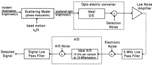
Generally, target spheres are very small, and only a few nanoWatts of scattered power can be collected (Figure 2-8). A photomultiplier tube is used because of its extremely high gain. A low noise amplifier amplifies the detected light signal. Finally, the signal is low-pass filtered and is captured by an analog-to-digital capture board. The data are stored on a computer and processed off-line.

(36)

Scattered Photomultiplier Low Noise Low Pass A/D

Light Tube Amplifier Filter Capture

Figure 2-8: The detection process.

2.3.1 Photomultipliers

A photomultiplier tube (PMT) is a sensitive device used to measure optical radiation.

The device consists of an evacuated cylinder containing a photoelectric cathode, a series of intermediate electrodes (dynodes), and an anode. When light enters through the aperture, it is absorbed by the cathode. This radiation excites electrons from the cathode's surface. These electrons are focused and accelerated through a potential field toward the first dynode. At the dynode, multiple electrons are emitted for each one that is absorbed. The electrons cascade through increasing dynode potentials and amplify the signal current. The anode collects the output power from the dynodes and drives an external load[4].

2.3.2 Noise Mechanisms

The output of a PMT is never perfectly proportional to the incident light due to noise factors. The optical power and dynode currents are carried by discrete carriers, each of whose behavior is governed by a random process. The variations in currents that this randomness introduces are called shot noise. The ratio of shot noise to signal rapidly decreases as the current becomes large because the variance of the mean of a number of independent events decreases with the number of events. Since far fewer carriers pass through the cathode than the dynodes, the cathode shot noise dominates the other sources of shot noise[4].

The current in the cathode is due to photon absorption as well as dark current. Dark current is present in the absence of illumination and is due to thermal noise and external radiation. The noise power observed at the output due to shot noise at the

(37)

cathode is

i = G2 2e(ic+ id)Av (2.19)

where G is the total PMT current gain, i is the signal current at the cathode, id is the dark current, and Av is the observation bandwidth[4]. The rms noise density is found to be

= G2e(iC + id). (2.20)

Another type of noise affects PMT operation because the anode current drives a load. The random motion of carriers in the conductor introduce Johnson (thermal) noise in the output signal. The observed Johnson noise power is

AN2 - 4kT (2.21)

N2

R

where T is the temperature and R is resistance of the external load[4].

2.3.3 Direct Detection

In direct detection, the incident optical power is the desired signal. The PMT pro-duces a signal current that is proportional to the incident optical power. Incident photons on the cathode stimulate electron emission. The quantum efficiency of the material is the average number of electrons emitted per absorbed photon. Consider the case where the time-average intensity of incident light is a raised, modulated cosine. The electric field incident on the detector is

es(t) = E,[1 + V cos(wmt)] cos(27rvt) (2.22)

where E, is the average electric field, V is the degree of amplitude modulation, wm is frequency of the modulation, and v, is the frequency of the incident light[4]. The photocathode current is given by

i~(t) =Pert 2.3

ic (t)

= v[1 + Vcos(Wmt)]2 _(2.23)

(38)

Pej V2

V2

= [(1

+

)+ 2Vcos(wt) + cos(2Wmt)] (2.24)

hv, 2 2

where P is the mean optical power incident on the cathode, 77 is the cathode quantum efficiency, h is Plank's constant, and e is the charge of an electron[4].

The combination of a signal AC frequency on a DC carrier yields three current frequencies at the detector: a DC component, an AC component at the incident frequency, and an AC component at twice the incident frequency. If the frequency range of incident signals is sufficiently band-limited, the undesired high frequency signals may be filtered out. If a PMT has an overall current gain of G, then the signal component of the output current will be

is(t) = Gic(t). (2.25)

The output of a PMT may be viewed as an equivalent circuit where the signal and noise sources appear as parallel current sources. Since the dynode shot noise is much less than the cathode shot noise, it may be neglected without significant error. Combining equations 2.19, 2.21 and 2.25 yields an overall signal to noise ratio at the

incident frequency, win, of

S G2_2V 2_(Pe _/hv

8)2

- = = - Peid 1hv _.G2( _(2.26)

N i2g

+2

G22e(iZc + id)AV + AkT ovIR*

Since the gains of PMT's are typically extremely large, the cathode shot noise dom-inates the thermal noise for ordinary temperatures and resistances. In the limiting case, the signal to noise ratio reduces to

S V2(Per/hv,)2

~: (2.27)

N e(Per/hv, + id)(

2.4 Noise Considerations

The primary sources of noise in the system are the photomultiplier and amplifier. Other electronic noise sources, such as thermal noise, analog-to-digital conversion

(39)

noise, and external EM interference are generally much smaller than the detection noise. Optical sources of noise, such as external light sources, stray radiation, and unwanted reflections, are minimized through a carefully controlled environment and the use of modulation techniques to reduce the influence of low frequency effects. The noise sources are generally white.

An estimate of the effects of noise can be obtained by analyzing the case of ampli-tude modulation. The smallest possible change in position that could be determined is where the change in power due to the position change is equal to that of the noise. Since the photomultiplier shot noise typically dominates the system noise, the min-imum detectable change may be found by analyzing the cathode noise. The noise current in the cathode is representative of the total amount of noise in the system. Additionally, the signal current at the cathode is the amount of detected power. As previously discussed, the effective modulation index of the system is the relative amount of the detected power that represents a small change in position. Setting the noise current (Equation 2.19) equal to the detected signal current (Equation 2.25) times the effective modulation index (Equation 2.18) yields

-8 a Ax

2e(ic + id)AV = ic-IJ(-)-I (2.28)

7r s a

where ic is the required signal current in the cathode to be able to detect a change of Ax in position. Typically, the required signal current is much greater than the dark current, so the id term may be ignored. Squaring both sides and solving for the required signal current results in

- 2r2eA

C = 32[J(ra)"X]2 (2.29)

The amount of detected power depends linearly on the observation bandwidth and inversely with the square of the required detectable percentage change in position. The amount of collected light by the cathode is linearly related to the cathode cur-rent either by the photomultiplier's cathode radiant sensitivity specification or by Equation 2.24.

(40)

As the amount of detected light increases, the photomultiplier's relative noise strength decreases. Therefore, it is important to double check that the amplifier noise and analog-to-digital conversion noise are dominated by the photomultiplier noise. If this assumption does not hold, the representative noise power used in Equation 2.28 must be adjusted accordingly.

(41)

Chapter 3 Application Model

This research describes a scalable detection system that can be adapted to a variety of spatial and temporal resolutions. One area of active research where this would be especially helpful is in the study of the tectorial membrane - a key component of hearing systems. Spherical beads may be unobtrusively attached to the membrane, and the system is optically transparent, so interferometric methods are well suited.

3.1 The Process of Hearing

The process of hearing involves converting acoustic waves from the environment into neural signals for the brain. Humans are sensitive to sound vibrations between approx-imately 20 and 20,000 Hz. In most mammals, the external ear flap, the pinna, collects and directs acoustical waves into the ear canal. The waves travel down through the canal until they reach the tympanic membrane. This membrane is a taught conical structure that separates the external ear from the middle ear.

The middle ear is an air filled cavity that is connected to the respiratory system

by the Eustachian tube. Two membranes, the round window and the oval window,

separate the middle ear from the inner ear. Three middle ear bones (the malleus, incus, and stapes) act as levers to transmit vibrations from the tympanic membrane to the inner ear. The malleus is connected to the tympanic membrane while the stapes is connected to the oval window[12].

(42)

fluid

flu ld

Figure 3-1: Lever model of the inner ear. The last of the middle ear bones, the stapes

(1), transmits pressure waves to two fluid-filled cavities (2). These waves induce

motion in the tectorial membrane (3) and embedded hair bundles (4). The relative motion of the hair bundles allows the sensory cells (5) to detect sound (Freeman [13])

The oval window and round window adjoin opposite apertures of the cochlea. The cochlea is a complex coiled structure that is filled with fluid. Essentially, the cochlea functions as a folded tube (the cochlear duct) with its top half (the scala vestibuli) connected to the oval window and its bottom half (the scala tympani) connected to the round window. A thin gelatinous membrane, the tectorial membrane, rests inside on a bed of sensory cells, the hair cells that rest on the basilar membrane.

As the stapes pushes and pulls on the oval window, pressure waves are transferred to the scala vestibuli, through the organ of Corti, and down the scala tympani to cause opposite motion in the round window. The tectorial membrane and basilar membrane vibrate relative to each other and the motion stimulates the hair cells.

Despite its prominent position in the system that transforms sound into mechan-ical motions of sensory receptor cells, little is known about the mechanics of the tectorial membrane. This is due at least in part to the intrinsic difficulty in experi-mentally testing the tectorial membrane. It is small, fragile, and transparent - which makes it a difficult target of study. Nevertheless, measuring the material properties of the tectorial membrane is important for understanding cochlear mechanics.

(43)

3.2 Determing Material Properties

A gel is essentially a mesh of macromolecules that retains vast amounts of water and

ions. The tectorial membrane is a gel that is approximately 97 percent water and three percent proteins and carbohydrates. When one pushes on the gel, the proteins are forced to distort from their rest positions. In effect, they act as a network of elastic springs. This model is valid as long as the forces on the gel are slow enough that the displacement of elastic springs can follow the forces.

When the motions are very fast, the elastic spring forces exerted by the proteins are much smaller than the dampening viscous forces exerted by the water molecules and ions trapped within the gel. Since audible vibrations vary from 20 Hz to 20 kHz, these viscous properties may play an important role in process of transferring vibrational energy to the hair cells.

There have been several investigations of the stiffness of the tectorial membrane. Abnet and Freeman developed a method of embedding a magnetic bead in the tecto-rial membrane and pushing on it with an electromagnet[8]. With this method, they measured the stiffness of a mouse tectorial membrane to be approximately 0.2 N/m for a 10 pm bead[8]. Yet the direct approach of pushing and watching can require motions that are much larger than those during normal hearing. One way to get around this problem is to not push at all.

Because of thermal energy present in any system, molecules and particles are in constant motion. In the gel structure, bond forces constrain this motion, but over small ranges, particles are still moving randomly about. This motion is called Brownian motion and is the driving force behind diffusion.

In the range where viscous forces dominate, the thermal energy of the system will cause a uniformly random amount of movement during a small time interval. Since viscous forces dampen velocity and do not depend on position, each particle will have a higher probability of moving farther from some initial position as the time interval increases. Yet, this drifting behavior cannot go on forever in a gel. Once a particle drifts a certain distance, the spring forces will be greater than the forces due

(44)

to the thermal bouncing of molecules. The motion of a particle will be constrained to a certain range over long periods of observation. Thus, the stiffness properties can be determined with accurate measurements of the range and variation of randomly driven motion of beads.

3.2.1 Modeling Brownian Motion

A spherical particle embedded in a gel may be modeled as a bead connected to an

elastic spring network immersed in a viscous medium. The average energy of the sphere is its thermal energy,

TE =-kT (3.1)

2

where k is Boltzman's constant and T is the temperature. At a neutral spring position (with no elastic forces), this manifests as kinetic energy. As the sphere moves in the elastic medium, it transfers kinetic energy to potential energy. The potential energy stored as elastic energy by the sphere position is

1

PE = -Kx 2 _(3.2)

2

where K is the elastic spring constant of the system and x is the deviation from a rest position.

The maximum average range of motion of the sphere will occur approximately where the average kinetic energy has been transferred to the elastic network. At this

characteristic point, the elastic forces will dominate and the sphere will not move any farther from its rest position. Combining equations 3.2 and 3.1 yields a characteristic distance of

k1T2

= (3.3)

The characteristic distance is approximately the average maximum distance that a sphere will travel under only the influence of thermal energy.

Sphere movement during Brownian motion is a random processes. A characteristic amount of time for a sphere to move may be thought of as the amount of time that a

(45)

particle will travel a certain distance with probability one half. Under the assumption of only viscous forces, the sphere movement is driven by diffusion. The diffusibility of a sphere in a viscous medium governs how fast the sphere moves and is found by

D = (3.4)

67rawlise

where qisc is the viscosity of the medium and a is the diameter of the sphere[14]. The viscosity of the gel is an unknown material property. Under diffusion, the probability distribution of a sphere is a time varying Gaussian[14],

1

p(x, t) = exp (-x 2_/4Dt). _(3.5)

The probability distribution may be interpreted as the probability that a sphere will move a distance, x, in a time period, t. The time period serves as a characteristic time scale for each bead size and range of movement. Approximately solving Equation 3.5 for the time it would take to move a characteristic distance, X112, with probability

one half yields[14]

2

t1/2 = . (3.6)

3.2.2 Modeled Range of Movement

For the purposes of estimating the range of motion of a bead connected to a spring network, the spring constant was estimated by assuming that it scales linearly with sphere diameter[15]. The reported stiffness of 0.2 N/m for a 10 prm diameter bead was linearly interpolated for each modeled bead size[8]. The viscosity of the surrounding medium was unknown. Since a gel is primarily water, for purposes of estimating characteristic times and distances it was estimated by assuming that the gel had approximately the same viscosity as water. The diffusibility for each bead size was estimated with these parameters from Equation 3.4.

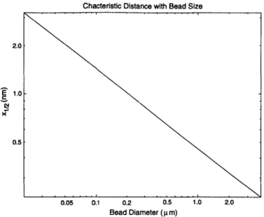
The characteristic distance scales inversely with the square root of bead diameter because the estimated spring constant (Equation 3.2) linearly increases with bead

(46)

Chacteristic Distance with Bead Size 2.0 E 1.0-0.5 0.05 0.1 0.2 0.5 1.0 2.0 Bead Diameter (p m)

Figure 3-2: Approximate range of bead movement at room temperature.

diameter. From Equation 3.3 the characteristic distance for a 0.1 Am diameter sphere was found to be approximately 1.4 nm, while the characteristic distance of a 1 Am diameter sphere was found to be 0.5 nm (Figure 3-2).

From Equation 3.6, the characteristic time depends on the square of characteristic distance, which scales inversely with diameter, divided by the diffusivity, which also scales inversely with diameter. Thus, the mode of characteristic time shows no net dependence on bead size. The characteristic time for this model was found to be approximately 0.4 Ms.

3.3 Modeling a Detection System

The idealized fringe based motion detector consisted of an illuminator, a detector, and a signal processor.

3.3.1 Target Illumination

We modeled the illumination system as two beams that intersect near their waists. Each beam had a wavelength (A, and A2) and a power. It was assumed that the

Broadband nanosensing using heterodyne interferometry