RESEARCH OUTPUTS / RÉSULTATS DE RECHERCHE
Author(s) - Auteur(s) :
Publication date - Date de publication :
Permanent link - Permalien :
Rights / License - Licence de droit d’auteur :
Institutional Repository - Research Portal
Dépôt Institutionnel - Portail de la Recherche
researchportal.unamur.be
University of Namur
Which Regional Policy Makes up for a Productivity Handicap?
Mignolet, Michel
Publication date: 2003
Document Version Peer reviewed version
Link to publication
Citation for pulished version (HARVARD):
Mignolet, M 2003, 'Which Regional Policy Makes up for a Productivity Handicap? Proceedings, ERSA, 2008'.
General rights
Copyright and moral rights for the publications made accessible in the public portal are retained by the authors and/or other copyright owners and it is a condition of accessing publications that users recognise and abide by the legal requirements associated with these rights. • Users may download and print one copy of any publication from the public portal for the purpose of private study or research. • You may not further distribute the material or use it for any profit-making activity or commercial gain
• You may freely distribute the URL identifying the publication in the public portal ?
Take down policy
If you believe that this document breaches copyright please contact us providing details, and we will remove access to the work immediately and investigate your claim.
European Regional Science Association ERSA 2003 Congress
University of Jyvaskyla, Finland 27th-30th August 2003
Which Regional Policy makes up for a
Productivity Handicap?
VERSION 2003.07.14
Michel MIGNOLET * CREW
University of Namur, Belgium
I. INTRODUCTION
Economic development is uneven over space. Regions are characterized by performance disparities in factor productivity: some regions are ahead, whereas others lag behind. The economic literature has stressed two main explanations, both relating to the firms’ location decision: endowments and externalities.1
Locational advantages result from differences in endowments between regions. While some attributes are present (possibly in abundance) in some regions, they are not present in other regions. Producers who value particular features will concentrate in locations with more of these attributes. This first explanation highlights that firms prefer to be near their inputs, either natural endowments (the presence of raw materials, access to sea, etc.) or local non traded infrastructure (roads, equipment in industrial parks, etc.). In any case, the effects of these two inputs mutually interact. Paraphrasing Lall, Shalizi and Deichman (2001), the benefits of a coastal location can be enhanced by the development of efficient seaports, and the costs of being landlocked can be reduced by investments in communication infrastructure, linking the hinterland to regions with access to harbours.
In addition, the concentration of economic activity is due to externalities. The literature distinguishes pecuniary externalities and production externalities. The former are analysed in the “new economic geography” models. Consumers are assumed to prefer a diversity of goods. To satisfy them, firms produce differentiated products in a setting of monopolistic competition and in the presence of increasing returns to scale and transportation costs (see, for example, Fujita and Thisse, 2002). Pecuniary externality models stress the strict preference of firms to be close to their customers and vice-versa.
Conversely, production externalities refer to the benefits to firms of proximity to other firms. These agglomeration economies are external to the firms. Following Marshall (1920) and Hoover (1936), it is now customary to consider two categories of production externalities. The co-location of firms engaged in similar activities generates so-called localization externalities2. These intra-industry benefits are notably attributable to knowledge spillovers
(by observing neighbouring firms and learning about what they are doing, firms acquire tacit and codified knowledge), a larger pool of specialized labour (there may be gains from locating in a “thick” labour market), and opportunities for efficient subcontracting. On the demand side, consumers take advantage of the reduction of information asymmetries and of a better quality/price ratio due to increased competition between suppliers. Of course, the benefits of own-industry concentration can be offset by negative externalities, such as the increased costs of labour, land and transport due to congestion. The empirical literature supports the presence of net positive effects from localization economies (see, for example, Ciccone and Hall, 1996 or Henderson, 2003). In addition, some benefits are expected from locating in close proximity to firms in other industries. These externalities arise from the scale or diversity of local activity outside the own-industry, involving a sort of cross-fertilization between firms (Henderson, 2003). They are called urbanization economies3 and are due to easier access to complementary services (advertising, specialized financial services, and
1 See for example LaFountain (2002).
2 Alternatively, in a dynamic context, Glaeser, Kallal, Scheinkman and Shleifer (1992) refer to these externalities
as Marshall, Arrow, Romer (MAR) externalities.
3 In a dynamic context, Glaeser, Kallal, Scheinkman and Shleifer (1992) refer to these externalities as Jacobs
publishing), and to a larger labour pool with multiple skills, as well as to inter-industry information exchanges and the availability of less-costly general infrastructure (Lall, Shalizi and Deichman, 2001). Again, these economies can be compensated for by costs such as increases in land rents and wage rates or commuting times for workers. Although the literature is not unanimous (see Henderson, 2003), since Sveikauskas (1975) evidence of net positive urbanization economies is most often reported.
The agglomeration process generates a snowball effect. A location with a high demand for a good attracts new producers, which in turn require additional employees. Workers can expect higher wages and a higher demand is then expressed for all goods at that location, making the region more attractive to other firms.
Whatever reasons are at work – differences in locational endowments and/or externalities – a unit of capital is expected to be diversely productive according to the region where it is installed. In addition, spatial disparities in land rents and wages are not bid away by firms and individuals in search of low cost or high income locations (see Henderson, Shalizi and Venables, 2001).
Regional policies have long been implemented in most industrialized countries with the purpose of achieving a better balance in the spatial distribution of economic activity. Generally speaking, regional policy relies on instruments that can be classified into two broad categories. The first range of instruments is aimed at directly increasing regional productivity by improving physical infrastructure (roads, telecommunications capabilities, etc.), human capital (education) or immaterial assets (R&D, consulting, etc.). The second category of instruments is more specifically designed to lessen the costs of factors by granting firms various capital (or labour) subsidies, providing fiscal incentives or lowering corporate tax rates.
A relevant question is whether the policy instruments are effective to offset a productivity handicap. In this paper, I focus particularly on the investment decision and on regional policies aimed at promoting capital formation in backward regions. I leave aside the instruments that affect other factors of production (the labour subsidies, for example). The purpose of this paper is to determine analytically to what extent some of the instruments (public capital stocks, capital grants, fiscal incentives and corporate tax cuts) must be implemented in order to make up for an unfavourable differential of productivity. The productive handicap that is common in lagging regions is considered to result from differences in agglomeration economies or in regional endowments.
The paper is organized as follows. Section II presents the basis model. A general expression is given that links together the cost of capital, investment incentives, public infrastructure, local endowments and agglomeration economies. By totally differentiating this expression, Section III determines analytically how high a particular instrument (an increase in a publicly provided input, a decrease of the tax base or of the corporate tax rate, or a capital subsidy) must be in order to offset an unfavourable differential of productivity. A numerical application is then developed in order to illustrate the approach and its relevance. Section IV addresses the question of the public cost associated with different instruments of regional policy in order to compare their relative performance. Section V concludes.
The private output in a region r is produced according to the following production function [1]: [1] α r r r r r r ) H a K )( G , F(K = Y
This expression is made up of three components. Since I am concentrating on the capital formation decision,4 the first term is a function F that combines privately owned capital, Kr,
and a publicly provided input, Gr. The latter term refers to any public spending (services to
enterprises, maintenance or setting up of infrastructure) that is under the control of government and that affects the firms’ productivity. Following Garcia-Milà and McGuire (2001), Gr, is supposed to be “distributed to firms in proportion to their capital stock” so that
the contribution of publicly provided inputs to the marginal productivity in region r is equal to [2]: [2] r G r r F' K G
where F’Gr represents the partial derivative of the function F with respect to the quantity of
publicly provided goods, Gr,in region r. Production in jurisdiction r is not only determined by
F but also by two other factors respectively linked to agglomeration economies and to endowment differences between regions.5
The first factor, (Kr/ar)α, is supposed to capture any productivity increase due to a greater
concentration of private capital, which arises from attempts to benefit from proximity either to the output market (as in pecuniary externality models), or to other firms in the same industry (to take advantage of the specialized know-how, with reference to localization externalities), or to firms in other industries (in order to exploit higher diversity and the mass effect, in relation to urbanization externalities). With reference to Ciccone and Hall (1996), K/a expresses the density ratio of private capital in an acre of space (symbolized by a) and α indicates the elasticity of output to density.
The second factor, Hr, is a Hicks-neutral shifter term that focuses any efficiency differential
over space that would be due to factors out of the control of the firm and of the public sector. It encompasses any locational advantage (or disadvantage) due to natural endowments (any gift of nature) or attributable to any inter-regional spillover effects. Whereas agglomeration economies due to information diffusion are known to decrease sharply with distance (Jaffe, Trajtenberg and Henderson, 1993) and, accordingly, are expected to produce no inter-regional spillover effect, the same is not true for some public infrastructure that may significantly affect private output outside the region where it is installed. Pereira and Roca-Sagales (2003)
4 All other arguments (notably labour, land and raw materials) are suppressed for simplicity. 5 That may not be totally reflected in factor prices so that market outcomes could be inefficient.
have given prominence to important spillover effects in Spain, with some regions benefiting greatly from public inputs being located elsewhere.6
Through agglomeration economies, each firm’s decision affects all firms outputs, including its own in the region. Following Garcia-Milà and McGuire (2002), none of the firms is assumed to take this into account.7 At the optimum, each firm chooses its capital stock so as to equalize the marginal contributions to production in value8 and the marginal cost of capital, as indicated in [3]: [3]
[
(ρ -π )+(δ-π )]
τ -1 ) A -(1 = H ) a K )( F' K G + (F' P P Kr r jr r r r α r r Gr r r Kr Kr rThe right hand side of equality [3] is the well-known expression of the gross-of-depreciation capital cost (see King and Fullerton, 1984). As Alworth commented, “it captures in addition to the financial cost, all other features of the tax system which might affect the investment decision of the firm, including depreciation allowance and a wide number of possible indirect investment incentives” (Alworth, 1988). It expresses the before-tax minimum rate of return that an investment project must yield in order to provide the saver with the expected net-of-tax return and to account for the loss of capital value due to depreciation. In this expression, πr
and πKr respectively symbolize the expected inflation rate for goods sold by the firm and the
real expected inflation rate on capital goods,9 δ is the exponential rate of economic depreciation,10 ρjr is the financial cost, τr is the corporate tax rate11 and Ar is the present
discounted value of any capital grant, tax credit or tax savings due to the allowances permitted for the asset, when the cost of the project is unity. In expression [3], all variables are possibly different between regions (they are noted with the subscript r) except δ that is supposed to be similar in each region.12
6 Some network infrastructure such as highways or telecommunications for example, is expected to have
important spillover effects. Positive spillover effects are not necessarily expected from some local ports or regional airports.
7 The aggregate amount of private capital is taken as a constant, when a firm makes its choice of capital and
labour (see Garcia-Milà and McGuire, 2001).
8 This is the gain to the firm from hiring an additional unit of capital. It is due to the marginal product of capital,
F’Kr, and to the marginal output from the increase in the publicly provided input, (Gr/Kr)F’Gr (see Oates and
Schwab, 1991). It is also attributable to any locational (dis)advantage, Hr(Kr/ar)α. 9 P is the price of output and P
K is the price of investment goods. πK is equal to
. .
P
Pk− where a dot over the letter indicates its rate of change.
10 (δ−π
k) expresses the effective economic depreciation rate accounting for the expected capital gain on capital
goods if P.k fP. . The literature generally states that δ is equal to 2/Le, where Le is the economic life of the
asset.
11 When the investment is cross-border, τ becomes a composite tax rate including the source and home countries
statutory tax rates on corporations, as well as any dividend withholding taxes, and taking into account the different methods for relieving double taxation.
12 The loss of value due to economic depreciation is clearly expected to be the same wherever the asset is
located. By and large, in this paper, the object is to compare the productivity of some neighbouring regions in a larger administrative entity. Accordingly, I shall consider that the variables concerning the general environment are identical for all regions. Notably, this is the case for the financing mix or, by assumption, for the general rules determining the proportions of the investment expenditure qualifying for tax allowances, which is entitled
The financial cost, ρjr, is the rate at which the firm discounts after-tax cash flows. It differs
according to the source of finance, j.13 Since nominal interest payments are tax deductible for the company, the financial cost for debt finance is ρDr = (1-τr) ir where ir is the interest rate. If
ψr expresses the nominal after-tax rate of return required by existing shareholders on retained
earnings, the financial cost of retaining profits ρRrt is equal to ψrt/ (1-mgr) where mgr is the
shareholders’ personal tax rate on capital gains (transformed into an effective rate on accruals). If one assumes that σr is the required return to new shareholders (which may differ
from ψr for generality), the financial cost associated with a new shares issue ρSr becomes [σr
+ πr (mgr-1+[1-mdr]θr) ] / θr[1-mdr], where θr denotes the opportunity cost of retained earnings
in terms of gross dividends foregone and and mdr symbolizes the personal tax rate on dividend
remittances [See King and Fullerton (1984) and Boadway and Shah (1995)]. θr is higher than
1 when methods of alleviating the economic double taxation of dividends (the imputation regime, for instance) are implemented.14 The term (mgr-1+[1-mdr]θr) is representative of the
net tax penalty attributable to the fact that a purely nominal return is taxed but escapes from any capital gain tax. King and Fullerton (1984) consider an arbitrage mechanism in such a way that the saver is indifferent between the three financing choices. In order to obtain this result the authors impose that ψr = σr + πr (mgr-1 + [1-mdr]θr) = (1-mir) ir where mir is the
personal tax on interest.
Expressions [4a], [4b] and [4c] summarize the financial costs for the three sources of finance: [4a] ρDr =(1-τr)ir when the investment is financed by debt;
[4b] ) m -(1 ) -1 ( gr r ir Rr i m =
ρ when the firm uses retained earnings; and [4c] r r Sr i θ ρ ) m -1 ( ) m -1 ( dr ir
= for new share issues.
If β is the fraction of the investment that is financed by debt, (1-β) is the proportion of equity finance, and ε is the proportion of equity finance from new share issues, the financial cost mix is provided by: [4d] ] ) m -(1 )i m -(1 ε) -(1 + )θ m -(1 )i m -(1 β)[ε -(1 + )i τ -β(1 = ρ gr r ir r dr r ir r r mr to immediate expensing or on which a capital subsidy can be granted. Of course, the degree of public generosity, the grant rate, for example, may vary between regions.
13 The expressions for the financial cost are more complicated when one considers cross-border financing. See
Alworth (1988).
14 Under the classical system of corporation tax, the tax liability of a company is independent of that of its
shareholders. No corporate tax is refunded when dividends are paid out, so the value of θ is unity. The two-rate system is the first method for allowing tax relief on dividends. Distributed profits are taxed at a lower corporate rate, τ, than retained earnings, which are taxed at the rate, τR. In this case, θ = (1+ τ- τR)-1. With the dividend
deduction system, companies are allowed to deduct x percent of gross dividends from the tax base. In this case, θ becomes equal to (1-xτR)-1. Finally, with an imputation system, a part of the company’s tax bill, say c, is imputed
to the stockholders. θ is equal to (1-c)-1. When full integration is granted, θ becomes equal to (1-τ)-1 [See
The left-hand side of expression [3] captures the productive contribution in value of one monetary unit of capital and the meaning of Hr has been explained above. (Pr/PKr)F’Kr and
(Pr/PKr)(Gr/Kr)F’Gr respectively measure the marginal productivity of private capital and the
marginal increase of output due to public inputs, in region r. Both terms are expressed in value per monetary unit.
III. ASSESSING THE IMPACT OF PUBLIC POLICY Expression [3] can be rewritten as follows:
[5] jr r kr Gr r r r r r r K
F
A a K H C [( ) ( )]'
1 1 ) ( 1 − + − − − − = − − ρ π δ π τ αwhere CKr = (Pr/PKr) F’Kr is the gross cost of capital in region r and F’Gr expresses the output
increase in region r due to any augmentation of publicly provided input. F’Gris equal to
(PrGr/PKrKr) F’Gr.
Following King and Fullerton (1984), public (regional) incentives may take one of three following forms: depreciation allowances, f1Adrτr, immediate expensing or any other device
aimed at decreasing the tax base, f2τr, and capital grants, f3sr.
[6] Ar = f1Adrτr + f2τr + f3sr
where f1, f2 and f3 respectively express the proportions of investment expenditure qualifying
for standard depreciation allowances, immediate expensing and grants. For the sake of simplicity, we assume that f1, f2 and f3 are identical whatever the region may be. Adrτr is the
present discounted value of tax savings from depreciation allowances; and sr is the rate of
capital grant, net of any corporate tax. Immediate expensing and tax allowances are devices that are expected to produce a similar effect on tax savings for an identical shock (an equal variation of f2 and of f1Adr). The former can take any continuous value. By contrast, the latter
refers to different patterns such as straight line, declining balance or other schemes allowed for tax depreciation, that yield discontinuous present values in terms of tax exemption. For the sake of simplicity, in the remainder of the paper I shall consider that any variation of f2 in
region r (df2r) is assumed to capture any (continuous) modification of the tax base due to
immediate expensing or tax allowance regimes.
By and large, public authorities use these fiscal (df2r) and financial (dsr) channels to stimulate
investment in lagging regions. Regional policy relies on two further instruments: lowering the corporate tax scale15 and financing public services to enterprises or infrastructure. What regional policy must be implemented in order to make up for an unfavourable differential of productivity? This question may be analytically addressed by examining how the gross capital cost is affected by the four following strategies: lowering the corporate tax rate, dτr,
decreasing the tax base, df2r, granting a capital subsidy, dsr, and providing public inputs, dGr.
Expression [7] gives the total differential of CKr. It measures the sensitivity of the capital cost
15 Temporary tax reductions on the corporate income, such as tax holidays, are a commonly used instrument in
with respect to these economic policies and to a variation of any productivity differential due to regional disparities either in externalities or endowments.
[7] ] ) / ( [ ] ) / ( [ 2 2 α α τ τ r r r r r r Kr r r Kr r r Kr r r Kr r r Kr Kr a K H d a K H C dG G C ds s C df f C d C dC ∂ ∂ + ∂ ∂ + ∂ ∂ + ∂ ∂ + ∂ ∂ =
From [7], it is easy to calculate the extent to which a particular policy is necessary to compensate a regional productivity deficit. In other words, I intend to measure the required variation in policy instruments dτr, df2r, dsr and dGr that maintain a constant capital cost (dCKr
= 0), notwithstanding the productivity differential.
[8a] α α τ τ [ ( / ) ] [ r( r / r) r Kr r r r Kr r C d H K a a K H C d ∂ ∂ ∂ ∂ = [8b] [ ( / ) ] [ ( / ) ] 2 2 α α r r r r Kr r r r Kr r d H K a f C a K H C df ∂ ∂ ∂ ∂ = [8c] [ ( / ) ] [ ( / )α] α r r r r Kr r r r Kr r d H K a s C a K H C ds ∂ ∂ ∂ ∂ = [8d]
[
α]
α ) / ( ] ) / ( [ r r r r Kr r r r Kr r d H K a G C a K H C dG ∂ ∂ ∂ ∂ =What alternative policies (dτr, df2r, dsr and dGr) are required to offset a handicap in the
productivity of a region r? In order to answer this question, we must solve each section of expression [8] to obtain the analytical expressions of dτr*, df2r*, dsr* and dGr*. When an
asterisk is associated with a policy variable, it indicates that the instrument exactly makes up for a regional productivity differential equal to
α ) r a r K ( r H d / )α r a r K ( r
H . Let us notice that this term is negative when the region faces a productivity handicap.
III.1. The analytical expressions of dτr*, df2r*, dsr* and dGr*
After some transformations, one obtains the expressions [9] to [12]:
[9]
[
]
1 3 2 1 1 2 Kr r r r * f -f -f -1 )] ( [ f f -) -( ) -( Ý -1 1 α ) r a r K ( r H α ) r a r K ( r H d − + + ∂ ∂ + ∂ + = r r r dr r dr r dr jr jr r s A A A d τ τ τ τ π δ π ρ τ ρ τ τwhere ρ ∂Ýjr τr,∂Adr ∂τr and some intermediary derivatives are detailed in the Appendix. In order to offset an unfavourable productivity differential in region r, public authorities have to modify the corporate tax rate by dτr*, as shown in expression [9]. The extent of dτr* is a
result of the product of the following two factors.
1. First, the productivity handicap that is to be compensated,
α ) r a r K ( r H d / )α r a r K ( r H ; and
2. Second, the inverse of the tax base on which the corporate tax is calculated. This tax base is obtained by algebraic summation of three terms: the required profit before corporate tax that yields one euro after tax, 1/(1-τr), adjusted to take into account the expected effect of
the variation of the corporate tax rate on the financial cost, ( ρÝjr ∂τr)/(ρjr -π r +δ -πKr), and on tax savings from immediate expensing and tax allowances, -r r r dr r dr r dr s A A A 3 2 1 1 2 f -f -f -1 )] ( [ f f τ τ τ τ ∂ ∂ + + .
In regard to df2r*, dsr* and dGr*, expressions [10] to [12] indicate the extent to which tax
incentives, capital subsidies or publicly provided inputs have to be implemented to offset a regional productivity handicap.
[10] 1 3 2 1 * 2 f -f -f -1 -α ) r a r K ( r H α ) r a r K ( r H d − = r r r dr r r A s df τ τ τ [11] 1 3 2 1 3 * f -f -f -1 f -α ) r a r K ( r H α ) r a r K ( r H d − = r r r dr r s A ds τ τ
[12]
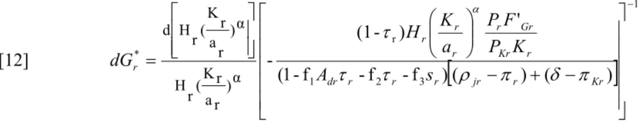
[
]
1 3 2 1 r * ) ( ) ( ) f -f -f -1 ( ' ) -(1 -α ) r a r K ( r H α ) r a r K ( r H d − − + − = Kr r jr r r r dr r Kr Gr r r r r r s A K P F P a K H dG π δ π ρ τ τ τ αExpressions [10] and [11] can be easily interpreted in the same way as [9]. The second factor expresses the corporate tax burden on which fiscal incentives are applied in [10] and the proportion of the asset qualifying for grants in [11], both being expressed by net euro invested.16 In expression [12], the last term indicates the after-corporate-tax additional output from the increase in the publicly provided input, taking into account the productivity differential, per net euro invested.
A numerical example will help us go further in the analysis. III.2. A numerical example
In order to illustrate the approach and its relevance, I shall consider the following scenario. The tax parameters are as simple as possible: a corporate tax rate, τ, is in force for distributed profits as well as for retained earnings and there is no double tax relief for dividends (the system is classical, with θ = 1). The corporate (τ) and personal (mi, mg, md) tax rates are close
to those used in some European countries or recommended by the European Commission (2001) or are used in some European countries and the pattern allowed for tax depreciation is the straight-line method. In this starting scenario, neither special fiscal provisions (such as a tax credit, f2) nor discretionary public aid (such as a capital grant, sr) is considered. The
investment is financed in equal portions by debt, undistributed profits and new share issue. The parameters characterizing the productivity disparities over space are calibrated so as to be neutral: Hr(Kr/ar)α is put equal to unity. The value assigned to the ratio Gr/Kr comes from a
statistical observation in the occidental economies and that attributed to F’Gr is inspired by
Pereira and Roca-Sagales (2003).
More precisely, the parameters take the values presented in Table 1. Table 1: The value of parameters in the starting scenario
The general tax parameters
f1 f2 f3 sr L τr mir mgr mdr θr
1 0 1 0 10 0.33 0.15 0 0.25 1
The parameters determining productivity disparity over space
Hr (Kr/ ar)α Gr/Kr F’Gr
1 0.04 0.085*
* This is the arithmetic average of the estimates of marginal products with respect to public capital inside the 17 regions in Spain (Pereira and Roca-Sagales, 2003, Table 3, p 250).
16 The cost of the investment is unity, minus the present discounted value of any tax allowances or grants given
The parameters characterizing the financing policy, inflation and depreciation rates
β ε Pr PKr πr πΚr Le i
1/3 1/2 1 1 0 0 L 0.05
In this scenario, the firm has a cost of capital net-of-depreciation that is equal to 6.39% and a financial cost of 4.42%. If region r faces a productivity handicap equal to 1% (that is d[Hr(Kr/ar)α]/[Hr(Kr/ar)α] = -0.01), what regional policy must be implemented in order to
make the firm equally profitable when location r is compared to other locations?
Table 2 shows to what extent the corporate tax rate must be changed, dτr*, or to what degree
an investment tax credit, df2r*, a capital grant, dsr*, or publicly provided inputs, dGr*, have to
be implemented in order to make up for this unfavourable productivity differential.
Table 2: The regional policy that must be implemented in order to make up for a productivity handicap equal to 1%
dτr df2r dsr dGr
- 0.024 + 0.0222 + 0.0073 + 0.0314
The productivity handicap in region r is fully offset when the corporate tax rate decreases by 2.4% to 30.6%, or if a tax credit of 2.22% is brought into play, a net-of-corporate-tax capital subsidy of 0.73% is granted or further public expenditures of 3.14 cents per unit of private capital are implemented.
IV. COMPARING REGIONAL POLICIES
In order to compare policies whose effects are rather different in kind and which are costly in various ways, let us measure the impact of each incentive on the public treasury.17 Accordingly, this brings to the fore the amount of public resources that have to be spent to balance a negative differential in productivity. For an investment project of one monetary unit, the cost associated with a capital grant or with publicly provided inputs is just equal to the amount of the capital subsidy itself or to the public expense per unit of private capital:
[13] Cs =dsr and CG =dGr
The cost of lowering tax rates, Cτ, corresponds to the tax revenue foregone on the income
from newly installed capital, throughout its whole lifetime:
[14] [ ] ) ( ) ( ) ( ) ( 0 Kr r gr Kr r u Kr r C d du e C d C gr r Kr π δ π ρ τ τ ρ π δ π τ − + − − = − =
∫
∞ − − + −where CKr e−[(ρgr−πr)+(δ−πKr)] expresses the nominal profits that increase with inflation, decrease
in value at the rate of depreciation, and are discounted at the public opportunity cost, ρgr.
Similarly, the cost of an investment credit (or of an immediate expensing), Cf2r, may be
expressed in terms of tax revenue foregone on the marginal investment income:
[15] Cf2 =τrdf2r
Which policy is less costly to be implemented in order to make up for a regional productivity handicap equal to 1%? Table 3 shows how costly are the four instruments of regional policy that have been considered, namely lowering the corporate tax rate, decreasing the tax base, granting a capital subsidy, and providing new public infrastructures. In order to measure Cτ, the public opportunity cost, ρgr, has been set at 4%.
Table 3: The costs associated with the four instruments of regional policy
Cτ Cf2 Cs CG
0.0264 0.0073 0.0073 0.0314 What are the main results? As shown in Table 3, granting financial aid or an investment credit
are the least costly policies. Both instruments require a public expense of 0.73 cents per euro of private capital, in order to make the firm equally profitable in spite of a 1% productivity handicap in region r.
Conversely, a lowering of the tax base appears to be a bad choice for the policy maker. It provides a weaker yield than the first two instruments. This outcome is easily explained. The benefits of a tax cut are actually lessened by the following double effect. On the one hand, a lower corporate tax rate proportionally reduces the tax savings due to the depreciation allowances and accordingly, lowers the net present value of Ar. On the other hand, it produces
a higher financial cost for the proportion of investment that is financed by debt.
Publicly provided inputs are even costlier. However, because they have the attributes, at least partly, of non-excludability and non-rivalness attributes18, these instruments may benefit a (potentially large) number of firms. Accordingly, it is impossible to conclude whether publicly provided inputs are a worse or a better public device in order to offset a regional productivity handicap.
V. CONCLUSIONS
Lagging regions are characterized by unfavourable differentials of productivity. This paper has investigated ways in which regional policies can make up for a regional productivity handicap. More precisely, four main categories of public aid have been examined: a lower corporate tax rate, an investment tax credit, a capital subsidy or publicly provided inputs. The results suggest that lowering the corporate tax rate is not an efficient policy tool. A subsidy net-of-corporate-tax and a decrease of the tax base produce similar effects for the
same cost. The setting up of new public infrastructure is costlier but generates productive externalities for a number of firms. It is difficult to determine a priori whether it is more effective than the other public instruments of policy.
In this paper, the opportunity of implementing a regional policy in order to offset some productivity handicaps has not been questioned. This matter is directly linked to some considerations in terms of equity and of optimal allocation. The former consideration brings to the fore the inter-regional distribution of wealth and is concerned with reducing disparities over space. The latter consideration is related to agglomeration economies. All firms experience productivity growth as the number or density of geographically concentrated firms increases. In order to achieve an efficient allocation, it is urged that these externalities be internalised by an adequate public policy.
REFERENCES
ALWORTH, J.S. (1988), The Finance, Investment and Taxation Decisions of Multinationals, Oxford: Basil Blackwell.
ASCHAUER, D. (1989), Is Public Expenditure Productive?, Journal of Monetary Economics, 23, 177-200. BOADWAY, R.W. and SHAH, A. (1995), Perspectives on the Role of Investment Incentives in Developing Countries, in A. SHAH, ed., Fiscal Incentives for Investment and Innovation, Oxford: Oxford University Press. CICCONE, A. and HALL, R.E. (1996), Productivity and the Density of Economic Activity, American Economic Review, 86, 1, 54-70.
EUROPEAN COMMISSION (2001), Company Taxation in the Internal Market, Brussels: European Commission.
FUJITA, M. and THISSE, J.-F. (2002), Economics of Agglomeration, Cambridge UK: Cambridge University Press.
GARCIA-MILA T. and McGUIRE T. (2002), Tax Incentives and the City, Brooking-Wharton Papers on Urban Affairs, 95-132.
GLAESER, E., KALLAL, H., SCHEINKMAN J. and SHLEIFER, A. (1992), Growth in Cities, Journal of Political Economy, 100, 1126-1152.
HENDERSON J.V. (2003), Marshall’s Scale Economies, Journal of Urban Economics, 53, 1-28.
HENDERSON J.V., SHALIZI, Z. and VENABLES A.J. (2001), Geography and Development, Journal of Economic Geography, 1, 81-105.
HOOVER, E. M. (1936), Location Theory and the Shoe and Leather Industries, Cambridge, MA: Harvard University Press.
JAFFE, A., TRAJTENBERG M. and HENDERSON, R. (1993) Geographic Localization of Knowledge Spillovers as Evidenced by Patent Citations, Quarterly journal of economics, 63, 577-598.
KING, M.A. and FULLERTON D. (1984) The Taxation of Income from Capital: A Comparative Study of the United States, the United Kingdom, Sweden, and the West Germany, Chicago Ill.: University of Chicago Press. LaFOUNTAIN, C. (2002), Where Do Firms Locate? Testing Competing Models of Agglomeration, Washington University, Mimeo.
LALL, S., SHALIZI, Z. and DEICHMANN U. (2001), Agglomeration Economies and Productivity in Indian Industry, Policy Research Working Paper 2663, The World Bank, August.
MARSHALL, A. (1920), Principles of Economics, 8th edition, London: Macmillan.
OATES, W.E. and SCHWAB R.M. (1991), The Allocative and Distributive Implications of Local Fiscal Competition, in D.A. KENYON and J. KINCAID, eds, Competition among States and Local Governments, Washington DC: The Urban Institute Press.
PEREIRA, A.M. and ROCA-SAGALES, O. (2003), Spillover Effects of Public Capital Formation: Evidence from the Spanish Regions, Journal of Urban Economics, 53, 238-256.
SVEIKAUSKAS L.A. (1975), The Productivity of Cities, Quarterly Journal of Economics, 89, 392-413.
APPENDIX
The sensitivity of financial cost with respect to the corporate tax rate The financial costs for the three sources of finance are equal to:
r )i -1 ( r Dr τ
ρ = , when the investment is financed by debt; ) m -(1 ) -1 ( gr r ir Rr i m =
ρ , when the firm uses retained earnings;
r r Sr i θ ρ ) m -1 ( ) m -1 ( dr ir
= , for new share issues where θr is equal to 1, r c -1 1 , r τ -1 1 , r gr τ τ + -1 1 or r xτ -1 1
, respectively under the classical, the partial or total imputation, the split-rate (or two-rate) and the deduction systems.
Let β be the proportion of new investment that is financed by debt. (1-β) is the fraction of equity finance. If ε is the proportion of equity finance from new share issues, the financial cost mix is provided by:
] ) m -(1 )i m -(1 ε) -(1 + )θ m -(1 )i m -(1 β)[ε -(1 + )i τ -β(1 = ρ gr r ir r dr r ir r r mr
The sensitivity of the financial cost with respect to the corporate tax rate is equal to: -i
= τÝ ρÝ
r
Dr , for debt issue and to =0
τÝ ρÝ
r
Rr , when the firm uses retained earnings. In case of
new share issue, the sensitivity of the financial cost with respect to the corporate tax rate is equal to =0
τÝ ρÝ
r
Sr , when the classical system or the partial imputation system is implemented;
and to ) m -(1 )i m -(1 -dr r ir , ) m -(1 )i m -(1 dr r ir and x ) m -(1 )i m -(1 -dr r
ir , for the total imputation regime, the
The sensitivity of tax allowances with respect to the corporate tax rate
Different patterns are allowed for tax depreciation. The present discounted value of tax allowances is given by the following expressions:
) e -(1 L ρ 1 = A -ρ L jr dl
jr , for the straight-line depreciation (L is the lifetime for tax
purposes); and jr dd ρ + u u =
A , for the declining-balance depreciation (u is the exponential rate at which the asset is depreciated).
Other schemes are allowed for tax depreciation, notably the declining-balance system with a switch to the linear regime. In this case,
] e -[e )ρ L -(L e + ] e -[1 b) + (ρ b = A -ρ L -ρ L jr s -bL b)L + (ρ -jr dz jr s jr s s jr , where L B = b , B is the
declining balance rate (equal to two for the double declining balance) and L B 1) -B ( =
Ls is the switchover point.
The sensitivity of tax allowances with respect to the corporate tax rate is given by the following expressions: ) τÝ ρÝ ( ρ L ) e -(1 -) τÝ ρÝ ( ρ ) (e = τÝ AÝ r jr 2 jr 2 L -ρ r jr jr L -ρ r dl jr jr
, for straight-line depreciation; ) τÝ ρÝ ( ) ρ + u ( u -= τÝ AÝ r jr 2 jr r dd
, for the declining balance; and
[
]
] ρ L) ρ -1 ( e -) L ρ -1 ( e ρ ) L -(L e + b) + (ρ 1] -1)e + b]L + [([ρ b) + (ρ b [ ) τÝ ρÝ ( - = τÝ AÝ jr jr L ρ -s jr L ρ -jr s bL -jr b)L + -(ρ s jr jr r jr r dz jr s jr s s jrfor the last depreciation scheme associating the declining balance and the linear regime.
The sensitivity of the capital cost with respect to the corporate tax rate, tax incentives, capital grants, publicly provided inputs and the regional productivity differential
α τ ρ τ τ τ τ τ τ τ π δ π ρ τ -1 -3 2 r 1 2 2 1 3 2 1 K ) ( )] Ý Ý ( ) -1 ( ) f -f -f -1 ( 1 ) ] ) Ý Ý ( [ ( 1 1 -( r r r r jr r r r dr r r dr r dr r r r r dr r r r jr r Kr a K H s A ) -τ ( f A A f ) -τ )-( s -f τ -f τ A -f ( ) =[ Ý ÝC + + + + α -r r 1 -r r K r jr r r 2 Kr ) a K ( H ) τ -1 ( )] π -δ ( + ) π -ρ [( τ -= fÝ CÝ r α -r r 1 -r Kr r jr 3 r Kr ) a K ( H ) τ -1 ( )] π -δ ( + ) π -ρ [( f -= sÝ CÝ r r r G Kr r r Kr K F' P P -= GÝ CÝ