Comparison of CFD simulations with experimental Jet Erosion Tests results

HAL Id: hal-01294936

https://hal.archives-ouvertes.fr/hal-01294936

Submitted on 30 Mar 2016

HAL is a multi-disciplinary open access

archive for the deposit and dissemination of sci-entific research documents, whether they are pub-lished or not. The documents may come from teaching and research institutions in France or abroad, or from public or private research centers.

L’archive ouverte pluridisciplinaire HAL, est destinée au dépôt et à la diffusion de documents scientifiques de niveau recherche, publiés ou non, émanant des établissements d’enseignement et de recherche français ou étrangers, des laboratoires publics ou privés.

P. Philippe

To cite this version:

Florian Mercier, Stéphane Bonelli, P. Pinettes, Frederic Golay, F. Anselmet, et al.. Comparison of CFD simulations with experimental Jet Erosion Tests results. Journal of Hydraulic Engineering, American Society of Civil Engineers, 2014, 33 p. �10.1061/(ASCE)HY.1943-7900.0000829�. �hal-01294936�

Postprint accepted - Journal of Hydraulic Engineering ASCE

Comparison of CFD simulations with

experimental Jet Erosion Tests results

Mercier F.(1),(2), Bonelli S.(1), Pinettes P.(2), Golay F.(3), Anselmet F.(4), Philippe P.(1)

(1)_{Irstea, 3275 Rte Cézanne, CS 40061, 13182 Aix-en-Provence Cedex 5, France}

(2)_{GeophyConsult, Savoie Technolac, 12 allée du lac de Garde, BP 231, 73374 Le Bourget du}

Lac Cedex, France

(3) _{Université de Toulon, IMATH, EA 2134, 83957 La Garde, France}

(4)_{IRPHE, Technopôle de Château-Gombert, 49 rue Joliot Curie, BP 146, 13384 Marseille}

Cedex 13, France

Abstract: The Jet Erosion Test (JET) is an experimental device increasingly used to quantify

the resistance of soils to erosion. This resistance is characterised by two geotechnical parameters: the critical shear stress and the erosion coefficient. The JET interpretation model of Hanson and Cook (2004) provides an estimation of these erosion parameters. But Hanson’s model is simplified, semi-empirical and several assumed hypotheses can be discussed. Our aim is to determine the relevance of the JET interpretation model. Therefore, we developed a numerical model able to predict the erosion of a cohesive soil by a turbulent flow. Our numerical model is first validated on a benchmark: erosion of an erodible pipe by a laminar flow. The numerical results are satisfactorily compared with the theoretical solution. Then, three JETs are modelled numerically, with values of erosion parameters obtained experimentally. A parametric study is also conducted to validate the accuracy of the numerical results and a good agreement is observed. The erosion parameters found experimentally permit to predict numerically the evolution of the erosion pattern within good accuracy. This result contributes to the validation of the JET’s semi-empirical model. The numerical model also gives a complete description of the flow, including vortices which can be observed in the cavity created by erosion. The whole erosion pattern evolution is given by the numerical results. Our numerical model gives information that is not available otherwise.

Keywords: Erosion, Jet Erosion Test, critical shear stress, erosion coefficient, turbulent flow,

Introduction

The Jet Erosion Test (JET) is a testing apparatus used to study soil resistance to erosion. The erosion is induced by a submerged circular turbulent jet impinging a sample of soil. This test was developed by Hanson (1990) and Hanson and Cook (2004). It enables quantifying the resistance of a soil to erosion via two geotechnical parameters. The first is the critical shear stress τc (Pa), which is the erosion threshold. The second is the erosion coefficient kd (m.s-1.Pa

-1

), that quantifies the erosion kinetics. The erosion rate of a soil is therefore equal to kd(τ −τc)

where ! is the shear stress exerted by the flow on the soil. The JET is currently the only test allowing the estimation of erosion parameters both in laboratory and in situ. In particular it has been used intensively, first in the USA and then in other countries for about ten years (Allen et al. 1997; Chang et al. 2011; Hanson and Hunt 2007; Karmaker and Dutta 2011; Lee et al. 2009; McClerren et al. 2012; Midgley et al. 2012; Pollen-Bankhead and Simon 2010; Thoman and Niezgoda 2008). The model interpreting the JET by Hanson and Cook (2004) uses the analytical approach of Stein et al. (1997) and the identification method of both erosion parameters has been recently refined by Pinettes et al. (2011). This is a simplified model which can be qualified as semi-empirical. It is especially based on the maximum shear stress exerted by a submerged jet impinging perpendicularly on a non-erodible flat plate. Hanson and Cook (2004) established a master equation which links geotechnical parameters, scour depth evolution and hydraulic parameters. This master equation is based on semi-empiric relations. During a JET, the evolution of the scour depth in function of time is measured. So, after the test, the pressure applied at the inlet of the experimental device and the scour depth evolution in function of time are known. Two unknowns are still remaining: the geotechnical parameters of the soil (the critical shear stress and the erosion coefficient).

parameters which permits to fit the best the experimental data is chosen. Geotechnical parameters are chosen so that the scour depth evolution obtained with the model fits the experimental data, they are fitted on the experimental results. To validate the accuracy of the erosion parameters found with the master equation, the development of a numerical model is needed. This model must be able to predict the erosion of a cohesive soil by a turbulent jet flow. As an input, the erosion parameters will be implemented and the evolution of the scour depth found numerically will be compared to the experimental results. If the final scour depths reached numerically and experimentally are within 30%, we will infer that the erosion parameters found with the Hanson’s semi-empirical model are relevant. The numerical modelling will then contribute to the validation of the JET interpretation model. Modelling numerically the erosion of a cohesive soil by a turbulent flow is a major challenge. Several studies present numerical models of erosion of granular soils by laminar flows (Papamichos and Vardoulakis 2005; Ouriemi et al. 2009), but none of them is suitable to cohesive soils submitted to turbulent flows. However, submerged impinging circular water jets have been vastly studied experimentally (Beltaos et al. 1974; Hanson 1990; Looney et al. 1984). A large number of semi-empirical formulas have been formulated on the basis of simplified models and measurements to characterise the evolution of different flow variables of a jet impinging on a non-erodible flat plate: the shear stress on the plate, the velocity field, and the static pressure. Nonetheless, although the geometry of this configuration is simple, it comprises highly complex physics due to the fluid mechanics involved, especially regarding the turbulence and flow close to the wall (Craft et al. 1993; Gibson et al. 1978). In addition, erosion modifies the surface of the soil by scouring it, forming a shape that depends on the jet and the resistance of the soil.

The purpose of present article is to contribute to the evaluation of the relevance of the model interpreting the JET. The method includes CFD (Computational Fluid Dynamics) numerical

simulations of JET, with the two erosion parameters τc and kd as input data. The numerical

results obtained are then compared to the experimental measurements that have been used to identify the erosion parameters. The system of equations used relies on the works of Bonelli and Brivois (2008), Bonelli et al. (2012), Golay et al. (2011). These works have shown that when the flow is strong enough, and when the soil is cohesive, erosion is sufficiently slow in comparison to the flow to allow neglecting the diphasic character of the phenomenon. Our numerical model addresses two major challenges: i) modelling the shear stress of a complex turbulent flow at the wall with accuracy; ii) modelling changes in geometry caused by the erosion.

In this paper, we first describe the numerical model. Then, our numerical model is validated on a benchmark: erosion of a pipe by a laminar flow with a constant pressure drop. The results obtained for the numerical modelling of three JETs are presented in the next section. Eventually, a discussion is proposed in the last section.

Numerical model

Modelling flow/erosion coupling

The intensity of erosion is characterised by the erosion number (Bonelli and Brivois 2008; Bonelli et al. 2012) in the same way as the Reynolds Number is used to characterise flow intensity. The erosion number is equal to ρkdV, where ρ is the density of the soil (kg.m-3

), kd

(m2

.s/kg) is the erosion coefficient and V is the average velocity of the flow causing erosion and transport. When this number is low (ρkdV! 1), the following hypotheses can be made:

i) If external conditions are such that the flow is stationary without erosion, then it remains stationary during erosion.

ii) The flow can be considered as a diluted suspension. The concentration of soil particles in the fluid is negligible and does not influence the flow.

In practice, cohesive soils have a density about 103 kg.m-3 with a JET erosion coefficient less than 10-4 _{m².s/kg. The average flow velocity close to the soil is of the order of 1 m.s}-1

. Consequently the erosion number is less than 10-1

. We can therefore make the assumption of slow erosion kinetics. It is then possible to simplify the model, since the only significant effect of erosion on the flow is the evolution of the soil-flow interface geometry (Bonelli et al, 2012).

Modelling a singular soil/water interface is a particularly complex task, since each medium is usually described using very different approaches: fluids are more naturally described by an Eulerian type model while solids are described by a Lagrangian type model. As it is necessary to determine the flow with accuracy close to the interface, especially the shear stress, a combined Euler-Lagrange method was chosen.

After performing temporal discretization, the computation is carried out in two stages at each time step:

i) The stationary flow is computed with a fixed flow/soil interface and the shear stress ! is evaluated,

ii) The geometry is then updated for the following time step as a function of the erosion law, which gives x(t+Δt )=x(t)+c_!Δt, where x(t) is a point of the flow/soil interface at the instant t, Δt is time step, and c_! is the celerity of the mobile interface noted !. The time step is estimated by a kind of CFL (Courant, Friedrichs, Lewy) method. It is calculated so that the maximal displacement of the nodes composing the interface can not exceed 10% of the adjacent cell size. This percentage was chosen to ensure a good stability of the numerical model.

Equations related to the flow

The flow is described by incompressible Navier-Stokes equations integrated by the finite volume method. The fluctuations of the unsteady flow are averaged statistically in order to obtain a stationary flow in conformity with the RANS (Reynolds Average Navier Stokes) method.

()

()

µ the molecular viscosity and _{10 kg m}3 -3

w= .

! the density of water, p the static pressure, T the Cauchy stress tensor,

w!"#u'u'

the turbulent stress tensor, often denoted Reynolds stress tensor R. The turbulent stress tensor is determined from the velocity fluctuations u' in relation to the average velocity u and ()Du, the symmetrical part of the average velocity gradient. Direct Numerical Simulations or Large Eddy Simulations are still too costly in terms of calculation time to model such an extended domain with high Reynolds numbers, added to remeshing problems.

The RANS closure problem is solved by a k -! turbulence model (Wilcox 1998). This turbulence model is known to be well adapted to impinging jet flows and to wall flows with streamwise pressure gradient or wall curvature.

The pressure/velocity coupling is solved by the use of the SIMPLE (Semi-Implicit Method for Pressure-Linked Equations) algorithm (Patankar and Spalding 1972). Spatial discretization is based on a second order accuracy upwind scheme (Barth and Jespersen 1989). Gradients are calculated with the Green-Gauss node based method (Rauch et al. 1991).

Erosion model

The erosion law is written in terms of the mobile interface celerity c_! which is related to the rate of local erosion:

( ) if 0 else d c c k c! ! ! ! ! " > = on ! (3)

with k the erosion kinetics coefficient, d c!

the critical shear stress and ! the norm of the shear stress on the interface defined by:

! _{= (T n? )}2 _{!(n T n? ? )}2 ₍₄₎

where n is the unit normal to ! oriented towards the soil.

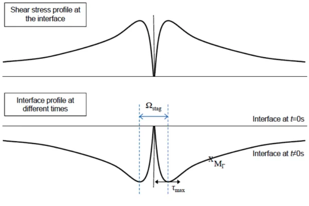
According to the erosion law Eq. (3), the displacement of a point of the interface depends only on the shear stress exerted by the fluid on the material at this point. In the case of a normal flow at the surface of the soil, the shear stress is null at the point of impingement, increases to its maximum and then decreases again by moving away from the stagnation zone (Fig. 1). As shown in Fig. 1, a geometric singularity appears in the stagnation zone that should be indicated by a peak of non-eroded soil. However, when carrying out the JETs, experimental observations relating to the shape of the eroded area showed that it did not fit the theoretical shape induced by the erosion law Eq. (3). Depending on the test, erosion was more or less deep and the diameter of the eroded area was more or less wide, but in no case was a central peak or a singular point at the center observed.

We assume that in the case of erosion by turbulent jet flow, the fluctuations of instantaneous values associated with the flow at the jet stagnation zone, as well as the pulse of the jet in 3D geometry, enable smoothing the peak of non-eroded soil in practice.

This stagnation zone of the jet flow Ωstag at the water/soil interface is defined between the jet

τmax is the shear stress at the outlet of the stagnation zone and the erosion law (1) can be

modified as written by Eq. (5).

max max stag

stag ( ) if in ( ) if out of 0 else d c c d c c k c k ! ! ! ! ! ! ! ! ! " > # = " > # (5)

This form of the erosion law remains valid whatever the configuration of the flow. Therefore in the case of a non-normal flow at the water/soil interface, Ωstag=Ø and Eq. (5) remains the

same as Eq. (3).

The numerical model is first validated on a benchmark. The erosion of a channel by a laminar flow with a constant pressure drop is modelled and the results are compared with the theoretical solution. Then three JETs performed on different soils are modelled. The numerical results are compared with the experimental and the semi-empirical ones.

Validation of the numerical model on a laminar case

The erosion of a cohesive soil by a laminar flow, in the well-known 2-dimensional Poiseuille flow configuration (Fig. 2), can be used as a benchmark to test our numerical modelling. The theoretical solution for the horizontal velocity of the flow u reads:

( )

_{( )}

( )

_{( )}

with R(t) the channel diameter at time t, u_av the average horizontal velocity and p the pressure field. The wall shear stress is deduced from the horizontal velocity:

( )

( )

For a constant pressure drop, the resolution of the erosion law in Eq. (3) gives (Bonelli et al. 2012):

( )

with R0 being the initial diameter of the erodible channel, t_er a characteristic erosion time

scale and L the length of the channel.

We set the following boundary conditions: R0=0.5 mm, L₂ =1 m and " =P 10 Pa!2 . The

erosion parameters are: k_d =10 m .s/kg!6 2 , !c=0 Pa. To ensure the independence of the

results from the mesh density, the mesh used is a uniform grid of 20x20,000 cells.

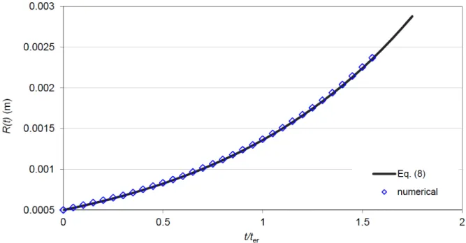
The numerical results obtained are compared with the theoretical solution of Eq. (8). As the pressure condition is imposed at the inlet, the erosion process never stops. On the contrary, the erosion accelerates exponentially through time, as described by the Eq. (8). Fig. 3 shows the evolution of the channel diameter as a function of dimensionless erosion time. A good agreement between numerical and theoretical results is obtained: in any time, the relative error is lower than 2%. These results validate our fluid-structure interactions numerical model. The Lagrangian interface movement model with remeshing is able to predict satisfactorily the erosion phenomenon. This validation is established for a laminar pipe erosion case, theoretical solution for turbulent impinging jets remains unknown. Therefore in the next section, we compared our numerical results obtained for turbulent flows to the experimental ones.

Jet Erosion Tests modelling

Characteristics of the soils tested

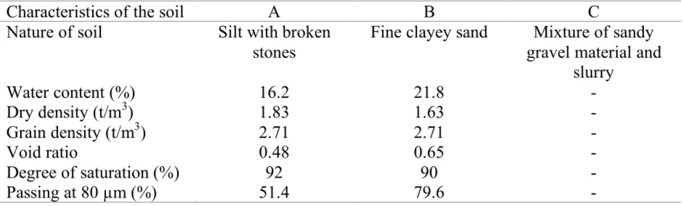
The three different soils tested with the JET tests, labelled respectively A, B and C were taken from existing dikes. The test protocol followed for these different erosion tests conformed to that of Hanson et al. (2004). Soil A is a clayey soil with a dry density of 1 83 10 kg m, . 3 . -3 and a water content of 16.2% volume. Soil B is a sandy soil with a dry density of 1 63 10 kg m, . 3 . -3

and a water content of 21.8% volume. The full results of the identification tests performed on test materials A and B are presented in Table 1. Soil C is a mixture of a sandy-gravel material and a mud composed of 69% water, 25% cement and 6% bentonite. The test was performed after 24h drying. No other characteristics of soil C are available.

The initial conditions applied for each test are presented in Table 2 and the notations used are explained in Fig. 4. The photographs of soil samples before and after the JET tests are shown in Fig. 5. The mould is 11.6 cm depth and its radius is 5.6 cm. The test data were interpreted using the equations of Hanson et al. (2004) and the identification method by Pinettes et al. (2011). The results obtained for the characteristic erosion parameters (erosion coefficient and critical shear stress) are given in Table 2.

These three tests were chosen for their differences in terms of soil type, final scouring depth and duration of the erosion process. However, the erosion parameters, critical shear stress and erosion coefficient of the materials tested are quite similar. Fig. 6 illustrates the differences observed experimentally on the scouring depths and erosion kinetics between the three tests. In the case of test B, the final scour depth is reached 10 times more rapidly than for test A. Their final scouring depths are about 5 and 6 cm respectively. In the case of test C the bottom of the mould in which the material was placed is reached rapidly. Fig. 6 also presents the

Results obtained for the three JETs

Whatever the JET modelled, the independence of the results regarding the mesh density is ensured to within 10%. At t=0 s, the meshes contain almost 70,000 cells. The soil/water interface is divided into almost 350 faces, whose lengths are about 10-4 m.

The results obtained numerically on the scour depths at the jet centerline are also shown in Fig. 6. The numerical results of the three tests are in good agreement with the experimental and semi-empirical results for the three tests. It can be seen in Table 3 that whatever the considered test, the error on the scour depth is lower than 25% for the comparison with the experimental results. The numerical results differ from the semi-empirical ones to 20% at maximum. Results obtained for the JET performed on soil B present the highest relative error on final scour depth and results on soil A the lowest. Concerning the erosion coefficient, the numerical results are also close to the experimental and the semi-empirical ones, especially given the time scale of the test. For the three tests, the time required to reach the final scour depth numerically is quite higher than the experimental one. With the erosion parameters found experimentally, our numerical model permits to find an evolution of scour depths within a good accuracy.

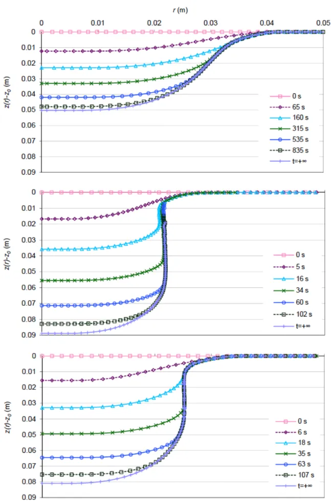
The evolution of the interface as a function of time for the three tests is presented in Fig. 7. The numerical results obtained for tests A, B and C are compared. The current experimental device does not allow the measurement of the whole interface position. Only the scour depth at the jet centerline is available. On the contrary, our numerical model gives the complete evolution of the erosion pattern and permits to visualize the flow inside and outside the eroded area. The curves show the evolution of the interface at some erosion times. For each graph in Fig. 7, the curves located at the greatest depths give the final state of the water/soil

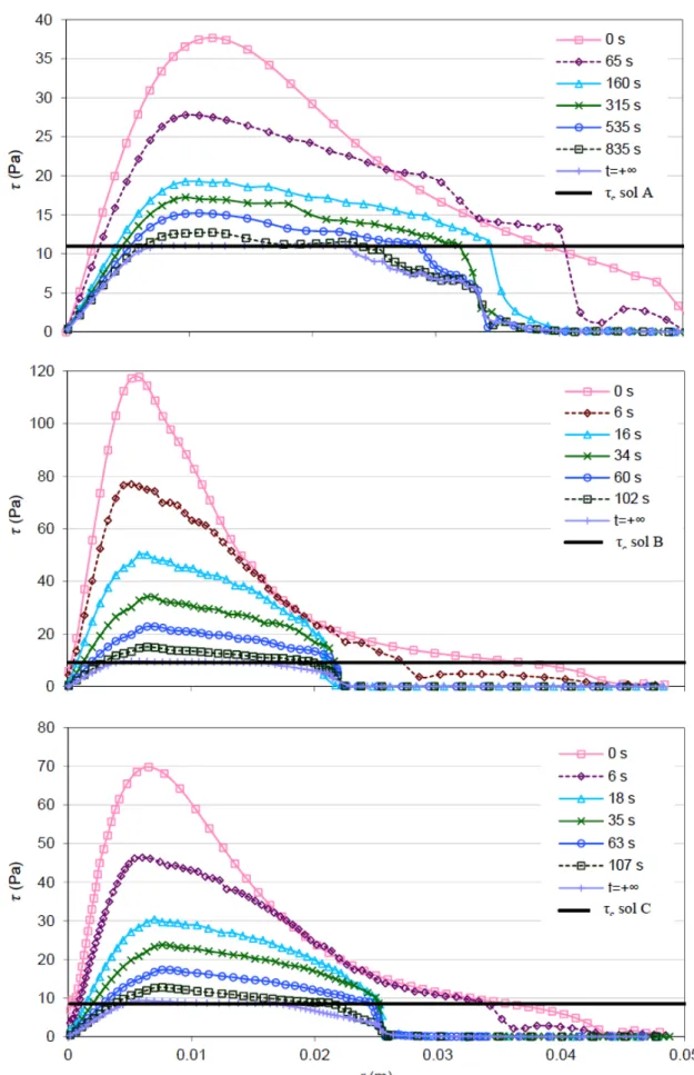
with the critical shear stress at every point of the interface. This can be seen in Fig. 8, which shows the results obtained for the evolution of the shear stress at the water/soil interface. Fig. 7 also shows in straight lines the threshold stresses specific to each test. The times selected correspond to those presented in Fig. 7.

Erosion developed differently for each of the three cases (Fig. 7). This difference can be attributed to the erosion parameters, as well as to the test conditions: pressure differential and initial distance between the nozzle and the soil, as given in Table 2. Although the soil erosion parameters are close for the three tests, the differences on pressure drops and nozzle/interface distances explain why scour depth evolutions are not similar for the three JETs. In the case of test A, the erosion affects a much larger zone than in cases B and C. In case A, the affected zone extends approximately up to r!4 cm, in case B, up to r!3 5 cm. and in case C only up to r!2 8 cm. . As shown in Fig. 8, the distribution of the shear stress at the water/soil interface at initial time points out the superposition of the areas affected by erosion and the areas for which c!!" in cases A and B. A difference is observed for case C, as the area where the shear stress is such that

c!!"

is larger than the area affected by erosion in reality. This can be explained by the fast reduction of the shear stress at the water/soil interface, as shown in the third graph of Fig. 8. Starting from the second curve of the evolution of shear stress on the water/soil interface, at a stage where erosion had hardly begun, the area for which c!!" is immediately reduced to r!2 8 cm. instead of r!3 8 cm. for the initial time. Similar reductions of shear stress can also be observed for the two other cases, but the intersection between curve

c!!=

and the first two evolution curves remains almost the same. As observed in Fig. 8, the values of the shear stress at the water/soil interface differ greatly from one test to another. The maximum shear stresses at the initial time are, for test A, about 37 Pa, for test B about 70 Pa, and for test C about 120 Pa. The pressure gradients imposed in

jet nozzle from the surface of the soil follow the same trend: for test C, the distance between the nozzle and the material is nearly 4 times less than that for test A, while for B it is nearly 2 times less than that for test A. The velocity of the fluid at the jet nozzle is about 7.8 m.s-1 in the case of test A and about 5.3 m.s-1 for the other two tests. The deceleration of the flow after the potential core of the jet (zone adjacent to the jet nozzle in which the velocity at the jet centerline remains constant) is inversely proportional to the distance between the nozzle and the considered ordinate. The velocity of the fluid just after the impact on the interface is nonetheless higher in case C in comparison to case B, and higher in the case of the latter than case A. The values of the different flow variables that are non-null at the water/soil interface, notably the shear stress exerted by the fluid on the material, are necessarily higher for test C compared to test B, and higher for test B than for test A.

The eroded areas of tests B and C are deeper than for test A. The maximum depth is about 5 cm for test A, about 8 cm for test B and about 9 cm for test C (see Fig. 6). As can be seen in Fig. 8, the maximum shear stress at the initial time in the case of test A is lower than that of test B, and lower in the case of the latter than that of test C. The highest shear stress values at the initial time lead to deeper scouring depths in the case where the critical shear stresses used for the different tests have very similar values. The distance of the nozzle from the water/soil interface increases progressively as the material erodes, leading to a decrease of shear stress on the interface. The erosion process stops when the shear stress becomes lower than the critical shear stress. Therefore for almost equal critical shear stress values, the higher the shear stress is at the beginning, the deeper the final erosion.

Fig. 9 shows the final shapes of the samples after erosion which are obtained numerically. A 2D view of the error made between the numerical and experimental results at the end of the erosion process for the JET performed on soil A is also shown. The difference is represented by the hatched zone between the two curves. The experimental results were obtained by direct

measurements on the soil sample after the test. In the most unfavourable case, i.e. at the jet centerline, the numerical results are still close to the experimental ones, with the error on scouring close to 14%. Although the erosion parameters are fitted with a flat plate semi-empirical model, the numerical results obtained for the entire erosion pattern are satisfactory. Also, the erosion shapes obtained numerically in the case of test B agree quite well with the photographs taken at the end of the test (Fig. 5). However, for test C the error is greater for the final scouring depth. We do not provide a numerical representation of reaching the bottom of the mould, at which point the side walls of the cavity formed by scouring usually collapse, as shown in Fig. 5. Nonetheless, Fig. 9 clearly shows the conclusions relating to the influence of the distribution of shear stress and the critical shear stress described previously.

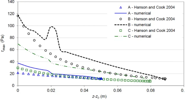
Fig. 10 shows the comparison between the numerical results and the semi-empirical model for the evolution of the shear stress for tests A, B and C as a function of the distance between the jet nozzle and the interface reached at the jet centerline. At initial time for tests A and B the numerical model gives results relatively far from those of the semi-empirical model of (Hanson et al. 2004). However, the results of the latter model are very close to those of our model at the initial time in the case of test C. For the three tests, an instability occurs at a depth of about 2 cm. It causes a substantial difference between the numerical and semi-empirical results in the case of test C. Whatever the considered test (after the instability in test C), we observed that the error between the numerical and semi-empirical results lessened as scouring depth increased. The curves related to tests A and B show a very similar stall at

0 2 cm

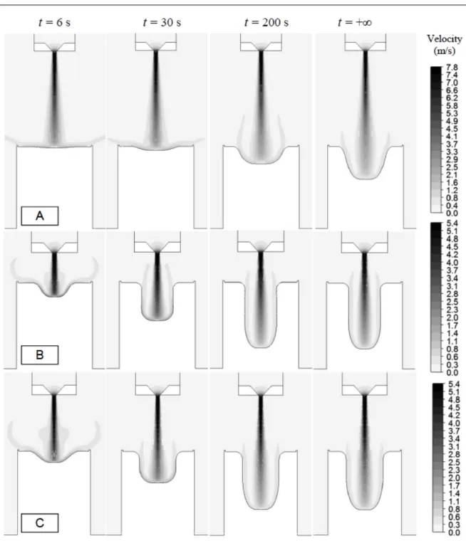
z z! = whereas test C presents a slightly different form of instability. The fact that the initial distance between the jet outlet and the water/soil interface is very close to the length of the theoretical potential core could also explain the formation of a slightly different instability in the case of test C. The numerical results obtained for tests A, B and C are also compared in Fig. 11, which presents the evolution of the velocity fields and the shape of the water/soil

interface as a function of time. The times are the same for each test in order to compare easily the different erosion kinetics. For each test of Fig. 11, the image at time t=15 000 , s gives the

final state of the water/soil interface. For a flat surface and for a slightly eroded water/soil interface, the impinging jet is deviated radially and in parallel to the surface, as shown by the first two pictures of the JET performed on soil A. The hollower the interface becomes, the more the flow at the outlet of the cavity is disturbed. Considerable zones of turbulence giving rise to the creation of vortices can be seen clearly on the first picture of tests B and C. For each of the tests, when the relative maximum depth reached is close to about 2 cm, the flow undergoes a change of regime and this time rises vertically and in parallel to the jet at the outlet of the cavity formed by erosion. This might explain the considerable disturbances at around 2 cm depth for the three tests shown in Fig. 10. Our numerical model permits to access flow characteristics which are not available elsewhere. The prediction of flow regime in the eroded areas and its evolution in function of time is first provided. Quantitative estimation of the role played by these vortices in the erosion process, in a way similar to the work performed by Hopfinger et al. (2004), will be the objective of more detailed analysis of the data obtained with the present numerical model.

Parametric study

To estimate the range of the erosion parameters for which numerical results are in good agreement with the experimental ones, a parametric study is carried out for test A. It permits to verify that the final scour depth is only dependent on the critical shear stress and that the erosion kinetics are a function of both erosion parameters. The parametric study also shows that the lower the erosion parameters, the higher the errors induced on the erosion kinetics or on the final scour depth are. An error of 50% on the erosion coefficient can lead to a

Likewise, an error of 100% on the critical shear stress leads to an error higher than 100% in asymptotic scouring depth. This demonstrates that the range of the erosion parameters for which numerical results are in good agreement with the experimental ones is narrow. Erosion parameters which are not at least of the same order of magnitude as those found with the interpretation model of Hanson can not permit to find a good agreement between numerical and experimental data. The erosion parameters found with the JET interpretation model within a range of few percent permits to track down the experimental results with a complex CFD numerical model. Our entry data were only the JET hydraulic parameters and the erosion coefficients obtained with Hanson’s fitting method. We implemented the entry data in our numerical model. And then we obtained the scour depth evolution in function of time. We compared this numerical data to the experimental ones, a good agreement is obtained. We also verified its reliability by a parametric study. The numerical model matches the experimental results; the Hanson and Cook (2004) model fits them. Our model takes the erosion parameters found by the semi-empirical method and verifies their accuracy. Therefore these results are a validation of the Hanson and Cook (2004) master equation.

Another approach is to find the numerical best fit of the experimental results. This study was performed with soil A. The entry data of the numerical model are then only the hydraulic parameters of the JET. We implement several sets of erosion parameters chosen arbitrary in our numerical model. We obtain then several scour depth evolutions in function of time. We compare them to the experimental data and we choose the set whose scour depth evolution fits the best the experimental data. And we found that the best set, which permits to obtain numerically the closest scour depth evolution to the experimental data, is very similar to Hanson’s optimal set: !c =9 Pa and

6 2

5 10 m .s/kg

d

k = . ! . Therefore we can deduce from these results that Hanson’s interpretation model of the JET is relevant, at least in terms of orders of magnitude and for this class of soils. Moreover, its shows that the semi-empirical

model gives accurate results within a very short calculation time. The numerical approach does not aim to replace the Hanson and Cook (2004) model nor to be more efficient. But it was needed to validate the objectionable assumptions on which the Hanson and Cook (2004) model is based.

Discussion

First, the discussion concerns the change in the flow regime, depending on the scour hole dimensions. The accuracy of this numerical result is supported by the experimental observations made by Aderibigbe and Rajaratnam (1996), Hollick (1976), Moore and Masch (1962). Depending on the scour hole observed at the end of the erosion process, two flow regimes are observed: the weakly deflected regime (WD) and the strongly deflected regime (SD). If the scour hole is wide and shallow, the WD regime is observed. On the contrary, if the scour hole is narrow and deep, the flow turns back to itself and SD regime is observed. At the current state of art, the transition between these two regimes is not yet clearly established. Then, Hanson’s semi-empirical model only takes into account the maximum value of the shear-stress on the interface. The shear stress model used is based on a flat plate assumption. Therefore, when the interface is eroded, digging the scour hole, it is expected that the error between numerical and semi-empirical results increases. On the contrary, the numerical results get closer to the semi-empirical ones with increasing erosion time. Despite the discrepancies observed in Fig. 10, the accuracy of the shear stress seems sufficient to obtain a good agreement of the results concerning the scour depth.

It is now possible to model the erosion of a cohesive soil by a turbulent flow with a simplified model and with reasonable computation requirements. This study shows that the characteristic parameters dk and c! , at least in terms of magnitude orders, permit to model the erosion

process within a good accuracy. This result is a validation of Hanson’s interpretation model, at least in terms of orders of magnitude and for this class of soils. Determining the range of the erosion parameters for which the model is validated requires additional cases modelling. Moreover, this study does not permit to validate the physical meaning of the erosion parameters. We imposed the erosion law in our numerical model. The implementation of another erosion law, with properly adjusted coefficients could also lead to numerical results in good agreement with the experimental ones. Considering the erosion law based only on the shear stress influence may not be justified and needs further considerable works to be validated or discredited.

Conclusion

A numerical model able to predict the erosion of a cohesive soil by a turbulent flow has been developed. It is first validated on a benchmark: the erosion of a channel submitted to a laminar flow, for which theoretical solution is known. Good agreement is obtained. Then, three JETs were simulated. The erosion parameters implemented in the CFD model were obtained from experimental data interpreted by Hanson’s semi-empirical model. The numerical results agree satisfactorily with the experimental results. The variations observed were of the same order of magnitude as the uncertainties usually encountered in soil mechanics with geotechnical parameters. A parametric study has been conducted to estimate the range of the erosion parameters for which numerical results are in good agreement with the experimental ones. Depending on the erosion parameters values, this range is always less than an order of magnitude. Therefore we deduce that despite its simplicity, the model of Hanson and Cook (2004) to interpret the JET results is relevant. Further work is still needed to determine the range for which erosion parameters are relevant and to determine the

physical meaning of the erosion parameters found with this erosion law. Moreover, our numerical model allows to access flow characteristics which are not provided with the semi-empirical model or with experiments. It leads to a better understanding of the flow regime inside and outside the erosion pattern. It can also provide access, in the future, to more detailed understanding of the phenomena involved in erosion, such as the specific role played by large-scale coherent vortices.

Acknowledgements

This study has benefit from support from the Hydraulic Engineering Centre of EDF. The authors of this publication would like to express special thanks to Messrs Jean-Robert Courivaud (EDF) and Jean-Jacques Fry (EDF) for their support and confidence. This work was also funded by the French National Research Agency (ANR) through the COSINUS program (project CARPEINTER No. ANR-08-COSI-002).

References

Aderibigde, O., and Rajaratnam, N. (1996). “Erosion of loose beds by submerged circular impinging vertical turbulent jets.” J of Hydraulic Research, 34(1), 19-33.

Allen, P. M., Arnold, J., and Jakubowski, E. (1997). “Design and testing of a simple submerged−jet device for field determination of soil erodibility.” Environmental and

Engineering Geoscience, 3(4), 579-584.

Barth, T. J., and Jespersen, D. (1989). “The design and application of upwind schemes on unstructured meshes.” Technical Report AIAA-89-0366, AIAA 27th Aerospace Sciences

Beltaos, S., and Rajaratnam, N. (1974). “Impinging circular turbulent jets.” J. Hydraulic Div., 100(10), 1313-1328.

Bonelli, S., Brivois, O. (2008). “The scaling law in the hole erosion test with a constant pressure drop.” International Journal for Numerical and Analytical Methods in

Geomechanics, 32, 1573-1595.

Bonelli, S., Golay, F., and Mercier, F. (2012). “Chapter 6 - On the modelling of interface erosion.” Erosion of Geomaterials, Wiley/ISTE, 187-222.

Chang, D. S., Zhang, L. M., Xu, Y., and Huang, R. Q. (2011). “Field testing of erodibility of two landslide dams triggered by the 12 May Wenchuan earthquake.” Landslides, 8(3), 321-332.

Craft, T., Graham, L., and Launder, B. (1993). “Impinging jet studies for turbulence model assessment – II. An examination of the performance of four turbulence models.” Int. J.

Heat Mass Transfer, 36(10), 2685-2697.

Gibson, M. M., and Launder, B. E. (1978). “Ground effects on pressure fluctuations in the atmospheric boundary layer.” J. Fluid Mech., 86, 491–511.

Golay, F., Lachouette, D., Bonelli, S., and Seppecher, P. (2011). “Numerical modelling of interfacial soil erosion with viscous incompressible flows” Computer Methods in Applied

Mechanics and Engineering, 200, 383-391.

Hanson, G. J. (1990). “Surface erodibility of earthen channels at high stresses part II – developing an in situ testing device” Transactions of the ASAE, 33(1), 132−137.

Hanson, G. J., and Cook, K. R. (2004). “Apparatus, test procedures and analytical methods to measure soil erodibility in situ.” Engineering in Agriculture, 20(4), 455-462.

Hanson, G. J., and Hunt, S. L. (2007). “Lessons learned using laboratory JET method to measure soil erodibility of compacted soils.” Applied Engineering in Agriculture, 23(3), 305-312.

Hollick, M. (1976). “Towards a routine test for the assessment of critical tractive forces of cohesive soils.” Transactions of the ASAE, 19(6), 1076−1081.

Hopfinger, E. J., Kurniawan, A., Graf, W. H., Lemmin, U. (2004). “Sediment erosion by Görtler vortices: the scour-hole problem.” Journal of Fluid Mechanics, 520, 327-342. Karmaker, T., and Dutta, S. (2011). “Erodibility of fine soil from the composite river bank of

Brahmaputra in India” Hydrological Processes, 25(1), 104-111.

Lee, L. T., Wibowo, J. L., Taylor, P. A., and Glynn, M. E. (2009). “In situ erosion testing and clay levee erodibility.” Environmental and Engineering Geoscience, 15(2), 101-106. Looney, M. K., and Walsh, J. J. (1984) “Mean-flow and turbulent characteristics of free and

impinging jet flow.” J. Fluid Mech, 147, 397-429.

McClerren, M. A., Hettiarachchi, H., and Carpenter, D. D. (2012). An investigation on erodibility and geotechnical characteristics of fine grained fluvial soils from lower Michigan.” Geotechnical and Geological Engineering, 30(4), 881-892.

Moore, W. L., and Masch, F. D. (1962). “Experiments on the scour resistance of cohesive sediments.” J. Geophysical Research, 67(4), 1437−1446.

Midgley, T. L., Fox, G. A., and Heeren, D. M. (2012). “Evaluation of the bank stability and toe erosion model (BSTEM) for predicting lateral retreat on composite streambanks.”

Geomorphology, 145, 107-114.

Ouriemi, M., Aussillous, P., and Guazzelli, E. (2009). “Sediment dynamics. Part 2. Dune formation in pipe flow.” Journal of Fluid Mechanics, 636, 321-336.

Papamichos, E., and Vardoulakis, I. (2005). “Sand erosion with a porosity diffusion law.”

Computers and Geotechnics, 32, 47–58.

Patankar, S. V., and Spalding D. B. (1972). “A calculation procedure for heat, mass ant

momentum transfer in three-dimensional parabolic flows.” Int. J. Heat Mass Transfer, 15, 1787-1806.

Pinettes, P., Courivaud, J.-R., Fry, J.-J., Mercier, F. and Bonelli, S. (2011). “First introduction of Greg Hanson’s « Jet Erosion Test » in Europe : return on experience after 2 years of testing.” Proc, 31st USSD Annual Meeting and Conference, 21st Century Dam Design -

Advances and Adaptations, San Diego, CA.

Pollen-Bankhead, N., and Simon, A. (2010). “Hydrologic and hydraulic effects of riparian root networks on streambank stability: Is mechanical root-reinforcement the whole story?”

Geomorphology, 116(3), 353-362.

Rauch, R. D., Batira, J. T., and Yang, N. T. Y. (1991). “Spatial Adaption Procedures on Unstructured Meshes for Accurate Unsteady Aerodynamic Flow Computations.”

Technical Report AIAA-91-1106.

Regazzoni, P.-L., Marot, D., Wahl, T., Hanson, G. J., and Courivaud, J.-R. (2008). “Soils erodibility: a comparison between the Jet Erosion Test and the Hole Erosion Test.” Proc.,

Inaugural International Mechanics Institute (EM08), ASCE, Minneapolis, MI.

Stein, O. R., and Nett, D. D. (1997). “Impinging jet calibration of excess shear sediment detachment parameters”. Transactions of the ASAE, 40(6), 1573−1580.

Thoman, R.W., Niezgoda, S. L. (2008). “Determining erodibility, critical shear stress, and allowable discharge estimates for cohesive channels: Case study in the powder river basin of Wyoming.” Journal of Hydraulic Engineering, 134(12), 1677-1687.

Wan, C. F., and Fell, R. (2004). “Investigation of rate of erosion of soils in embankment dams.” Journal of Geotechnical and Geoenvironmental Engineering, 30(4), 373-380. Wilcox, D. C. (1998). “Turbulence Modeling for CFD.” DCW Industries, Inc., La Canada,

Table 1. Identification tests on different soils subjected to JET tests.

Characteristics of the soil A B C

Nature of soil Silt with broken

stones Fine clayey sand gravel material and Mixture of sandy slurry Water content (%) 16.2 21.8 - Dry density (t/m3_{) 1.83 1.63 -} Grain density (t/m3) 2.71 2.71 - Void ratio 0.48 0.65 - Degree of saturation (%) 92 90 - Passing at 80 µm (%) 51.4 79.6 -

Table 2. Characteristic parameters of the Jet Erosion Tests modelled.

Parameters settled for the JETs numerical models A B C

Pressure differential (Pa) 30,000 15,000 14,000

Initial distance of jet nozzle from soil surface (cm) 14.6 4.1 7.8

Critical shear stress τc (Pa) 11.0 9.1 8.5

Erosion coefficient kd (m².s/kg) 1.0×10-5 4.5×10-5 7.2×10-5

Table 3. Relative error of numerical results in comparison to experimental results for the three tests.

Error on the final scour

depth in comparison to: A B C

Experimental results 14.5% 24.0% 20.1%

Fig. 1. Shear stress profile at the water/soil interface and erosion figure at different times calculated with Eq. (3).

Fig. 3. Results obtained for the numerical modelling of the erosion of a channel by a laminar flow.

Fig. 5. Surface of the soil sample before (a) and after (b) the Jet Erosion Test in the case of test A, B and C.

Fig. 6. Numerical results of JET tests A, B and C compared to the Hanson’s semi-empirical model fit and to experimental results, scour depth in function of time.

Fig. 8. Evolution of the shear stress along the water/soil interface as a function of time: test A at the top, test B in the middle and test at the bottom.

Fig. 9. Comparison of numerical results on the shape of the scour hole, case of tests A, B and C, experimental results are provided for test A.

Fig. 3. Comparison of numerical results and the Hanson’s semi-empirical model on the evolution of the norm of the shear stresses for tests A, B and C.

Fig. 11. Velocity field and profile of the water/soil interface as a function of time, in the case of JET tests A (top), B (middle) and C (bottom).