HAL Id: inria-00070194
https://hal.inria.fr/inria-00070194
Submitted on 19 May 2006
HAL is a multi-disciplinary open access archive for the deposit and dissemination of sci-entific research documents, whether they are pub-lished or not. The documents may come from teaching and research institutions in France or abroad, or from public or private research centers.
L’archive ouverte pluridisciplinaire HAL, est destinée au dépôt et à la diffusion de documents scientifiques de niveau recherche, publiés ou non, émanant des établissements d’enseignement et de recherche français ou étrangers, des laboratoires publics ou privés.
A library of Taylor models for PVS automatic proof
checker
Francisco Cháves, Marc Daumas
To cite this version:
Francisco Cháves, Marc Daumas. A library of Taylor models for PVS automatic proof checker. [Re-search Report] RR-5831, INRIA. 2006, pp.18. �inria-00070194�
ISRN INRIA/RR--5831--FR+ENG
a p p o r t
d e r e c h e r c h e
Thème SYM
A library of Taylor models for PVS automatic proof
checker
Francisco Cháves — Marc Daumas
N° 5831
Francisco Ch´aves, Marc Daumas Th`eme SYM — Syst`emes symboliques
Projet Ar´enaire
Rapport de recherche n 5831 — Jan 2006 —18pages
Abstract: We present in this report a library to compute with Taylor models, a technique extending interval arithmetic to reduce decorrelation and to solve differ-ential equations. Numerical software usually produces only numerical results. Our library can be used to produce both results and proofs. As seen during the devel-opment of Fermat’s last theorem reported by Aczel 1996, providing a proof is not sufficient. Our library provides a proof that has been thoroughly scrutinized by a trustworthy and tireless assistant. PVS is an automatic proof assistant that has been fairly developed and used and that has no internal connection with interval arithmetic or Taylor models. We built our library so that PVS validates each result as it is produced. As producing and validating a proof, is and will certainly remain a bigger task than just producing a numerical result our library will never be a replacement to imperative implementations of Taylor models such as Cosy Infinity. Our library should mainly be used to validate small to medium size results that are involved in safety or life critical applications.
Key-words: PVS, program verification, interval arithmetic, Taylor models.
This text is also available as a research report of the Laboratoire de l’Informatique du Paral-l´elisme http://www.ens-lyon.fr/LIP.
Une biblioth`
eque sur les mod`
eles de Taylor pour
l’assistant automatique de preuves PVS
R´esum´e : Nous pr´esentons une biblioth`eque sur les mod`eles de Taylor, une exten-sion de l’arithm´etique d’intervalles. Les logiciels num´eriques produisent usuellement des r´esultats num´eriques. Notre biblioth`eque peut ˆetre utilis´ee pour produire `a la fois des r´esultats et des preuves. Nous l’avons vu pendant le d´eveloppement du dernier th´eor`eme de Fermat retrac´e par Aczel 1996, fournir une preuve n’est pas suffisant. Notre biblioth`eque fournit une preuve qui a ´et´e contrˆol´ee dans les moin-dres d´etails par un inlassable assistant digne de confiance. PVS est un assistant automatique de preuve qui a ´et´e largement d´evelopp´e et utilis´e et qui n’a aucune re-lation interne avec l’arithm´etique d’intervalles ou les mod`eles de Taylor. Nous avons construit notre biblioth`eque de fa¸con que PVS valide chaque r´esultat au moment o`u il est produit. Comme produire et valider une preuve, est et restera certainement travail beaucoup plus important que produire uniquement un r´esultat num´erique, notre biblioth`eque ne saurait ˆetre un repla¸cant des implantations imp´eratives des mod`eles de Taylor comme Cosy Infinity. Notre biblioth`eque devra ˆetre r´eserv´ee `a la validation de codes petits `a moyens utilis´es dans des applications critiques ou qui pourraient compromettre des vies humaines.
Mots-cl´es : PVS, v´erification de programme, arithm´etique d’intervalles, mod`eles de Taylor.
A library of Taylor models for PVS automatic proof
checker
1Francisco Ch´aves2 and Marc Daumas3
Laboratoire de l’Informatique du Parall´elisme UMR 5668 CNRS–ENS de Lyon–INRIA email: [email protected]
Laboratoire d’Informatique, de Robotique et de Micro´electronique de Montpellier UMR 5506 CNRS–UM2
email: [email protected]
Visiting Laboratoire de Physique Appliqu´ee et d’Automatique EA 3679 UPVD
email: [email protected]
1
Introduction
Taylor models, see for example (Makino and Berz[2003]) and references herein, have recently emerged as a nice and convenient way to reduce decorrelation in interval arithmetic (Moore [1966];Neumaier [1990]; Jaulin et al.[2001]). Taylor models are even more attractive when one solves initial value problems ODEs as they provide a validated built-in integration operator.
Yet, it is now beyond doubt that programs and libraries contain bugs, no matter how precisely they have been specified and how thoroughly they have been tested (Rushby and von Henke [1991]; Ross [2005]). As a consequence, the highest Com-mon Criteria Evaluation Assurance Level, EAL 74, has only been awarded so far to
products that provide validation using a formal tool, specifically an automatic proof checker in first or higher order logic.
1
This text is also available from HAL https://hal.ccsd.cnrs.fr/ccsd-00018529 and arXiv
http://fr.arxiv.org/abs/cs.MS/0602005repositories.
2
This material is based on work supported by the Mathlogaps (Mathematical Logic and Appli-cations) project, an Early Stage Research Training grant of the European Union.
3This work has been partially supported by PICS 2533 from the French National Center for
Scientific Research (CNRS).
4
4 Francisco Ch´aves and Marc Daumas
We present here our library of Taylor models in PVS (Owre et al.[1992]). Work-ing with an automatic proof checker, we had to manage two tasks. The first task was to create a data type and operations on this new type to allow users to de-fine and evaluate expressions using Taylor models. The second task was to provide proofs that each operator is correct and a strategy to recursively analyze compound expressions. Both tasks rely on the recently published library on interval arithmetic for PVS (Daumas et al. [2005]). As many mathematical developments are not yet available in PVS, we also had to develop an extended library on polynomials and prove a few theorems of analysis and algebra.
Our library on Taylor models can be used to derive quickly more or less accurate bounds. For example, users of formal tools have to provide proofs that radicals are non negative for all expressions using square roots. Some proofs use intricate analysis but most of them are very simple and interval arithmetic or low degree evaluations with Taylor models can produce appropriate proofs. Our library can also be used to expertly derive computer validated proofs of difficult results through an expert use of Taylor models.
The library will be available freely on the Internet as soon as it is stable. Side developments are integrated as they are produced to NASA Langley PVS libraries5.
Meanwhile, all files can be retrieved from the author’s website.
http://perso.ens-lyon.fr/francisco.jose.chaves.alonso/pvs-files/
1.1 Working with an automatic proof checker
Software is used extensively for a wide array of tasks. Some pieces of software should never fail. The ones used by transportation means (planes, buses, cars. . . ), for medical care (controlling pumps, monitors, prescriptions. . . ) or in the army (parts of weapons, alarms. . . ) belong to the fast lengthening list of life or safety critical applications. A mindless modification of one parameter reportedly caused human losses in the Instituto Oncologico Nacional on Panama where eight people died and twenty others were hurt (Gage and McCormick [2004]). Many lethal and costly failures (Information Management and Technology Division[1992];Lions and others[1996]) show beyond reasonable doubts that traditional software verification is not sufficient to guarantee correct behavior.
PVS6 (Prototype Verification System) byOwre et al. 1992;2001a;2001bis one environment for the development and analysis of formal specifications that allows
5
http://shemesh.larc.nasa.gov/fm/ftp/larc/PVS-library/pvslib.html.
6
http://pvs.csl.sri.com/.
the elaboration of theories and proofs. The system deals with theories where users develop definitions, axioms and theorems. To verify that theorems are correct, PVS uses a typed higher order logic language where new types are defined from a list of basic types including booleans, natural numbers, integers. . . The type system allows the definition of functions, registers, tuples and abstract data types.
PVS uses predicate subtypes, subtypes where all objects satisfy a given predicate. For example {x : real|x 6= 0} is the set of non–zero reals. Subtype predicates are used for operations that aren’t defined for all possible inputs. This restriction is therefore visible in the signature of the operation. For example the division is an operation of real numbers such that the type of the denominator is a real number different from zero. As a result, all functions of PVS are total in the sense that the domain and the signature must exclude explicitly any input where a function could not be defined.
As predicates used by the system to define types are arbitrary, type verification is undecidable and it usually generates proofs obligations named type correctness conditions (TCCs). Users have to provide proofs of generated TCCs with the help of PVS.
In PVS the λ operator defines anonymous functions. Expression λx.e is a func-tion that has parameter x and returns expression e. For example, the funcfunc-tion that returns 0 for any value of its single parameter could be defined as λx.0 and identity function that returns the same element that is given as parameter is λx.x. Function λ k : nat. if k = 0 then 1 else 0 is the sequence that for input 0, returns 1, and returns 0 for any other input.
Nowadays, systems such as PVS are fully able to certify that programs are cor-rects (Ross[2005]) but programmers scarcely use them. Providing a formal proof of correct behavior is a difficult task, it requires a specific training and user interfaces of proof assistants are of little help for all the work that is not done automatically. Hope is that as more and more work is done automatically, users will need only limited interactions with automatic proof checkers down to the point where no interaction is required at all. This trend was recently coined as invisible formal methods (Tiwari et al. [2003]).
1.2 A few words about interval arithmetic
In interval arithmetic scalar variables x are replaced by pairs (a, b) with the semantic that x lies in the interval [a, b]. Later on, we compute bounds rather than values. We use operators commonly found in programming languages such as addition,
6 Francisco Ch´aves and Marc Daumas
subtraction, multiplication and so on (Jaulin et al.[2001]). [a, b] + [a0, b0] = [a + a0, b + b0]
[a, b] − [a0, b0] = [a − b0, b − a0]
c · [a, b] = [c · a, c · b] c ≥ 0
[a, b] · [a0, b0] = [min{aa0, ab0, ba0, bb0}, max{aa0, ab0, ba0, bb0}]
Working with automatic proof checkers, we convert operations into properties (Daumas et al.[2005]).
For all x ∈ [a, b], y ∈ [a0, b0] and c ∈ R
x + y ∈ [a, b] + [a0, b0] x − y ∈ [a, b] − [a0, b0] c · x ∈ c · [a, b] x · y ∈ [a, b] · [a0, b0]
Decorrelation is a problem intrinsic to interval arithmetic. There is decorrelation on interval evaluation of any expression where one or more variables appear more than once. For example, the most simple scalar expression
x − x
where x ∈ [0, 1], is replaced in interval arithmetic by
[0, 1] − [0, 1] = [−1, 1].
Everyone agrees that x − x lies in the interval [0, 0] but interval arithmetic pro-duces the correct but very poor [−1, 1] interval. Decorrelation and other problems lead interval arithmetic to overestimate the domain of results. Techniques are used intensively to produce constrained results.
One of such techniques is based on Taylor’s theorem with Lagrange remainder where f is n times continuously derivable between x0and x, f is n+1 times derivable
strictly between x0 and x and 0 < θ < 1.
f (x) = f (x0) + (x − x0)f0(x0) +(x−x0) 2 2! f00(x0) + · · · + (x−x0)n n! f(n)(x0) + (x−x0)n+1 (n+1)! f(n+1)(x0+ (x − x0)θ) INRIA
Adapting Taylor’s theorem to interval arithmetic, we obtain the formula below ( Dau-mas et al.[2005]) for x and x0 in I.
f (x) ∈ f (x0) + (I − x0)f0(x0) +(I−x0) 2 2! f00(x0) + · · · + (I−x0)n n! f(n)(x0) + (I−x0)n+1 (n+1)! f(n+1)(I)
Using Taylor’s theorem was appropriate in (Daumas et al. [2005]) but it has many drawbacks:
It is difficult to hide the use of Taylor’s theorem in order to provide invisible formal methods. This is due to the large number of quantities involved in instantiating the theorem in its generic form. Progress has been achieved by Mu˜noz after the publication of Daumas et al..
To use Taylor’s theorem, one has to express the derivatives of function f . For large expressions, f alone might be too large to be expressed in PVS. Taylor models presented in the rest of this text overcome all the previous draw-backs to the price of a less accurate approximation. We have developed a set opera-tions for PVS that includes addition, negation, scalar multiplication, multiplication, reciprocal and exponential. We present our developments in PVS, first quickly on polynomial functions and then on Taylor models. We finish with concluding remarks and a few toy examples.
2
Implementing polynomials in PVS
For the implementation of polynomials we considered a finite list of monomial func-tions, a finite sequence of coefficients and an infinite power series with finite support. Finite lists or sequences usually imply the construction of a new inductive type `a la Coq7 (Bertot and Casteran [2004]). We implemented polynomials as power series with finite support. This scheme is appropriate for a proof system like PVS and is compatible with NASA series libraries8.
Working with sequences of coefficients rather than monomial functions means that we need the powerseries function to evaluate polynomial P on input x. It
7
See for examplehttp://www.lfcia.org/staff/freire/phd-gilberto/gilberto_phd_html/.
8 Francisco Ch´aves and Marc Daumas
also means that some theorems can be established on finite support series rather than polynomial functions.
2.1 Finite support series
Our implementation of polynomials is outlined in Figure 1. It mostly describes mathematical objects (definition, function, theorems...) with common words except for the notions introduced in Section1.1
We define predicate finite_support (a,N) just after the preamble. Addition of sequences was already defined and is imported from previous work in the preamble. We had to define a product operator and a composition operator. The first operator applies to generic series. The second operator requires that the first sequences a returns zero for indices above input d.
In the second half of Figure1we proved that negation, addition, multiplication by a scalar, multiplication and composition return finite support series provided (both) inputs are finite support series. We also proved that Cauchy’s product is meaningful for finite support series. The meaning of composition can only be assessed in regard to polynomial functions.
2.2 Polynomial
As we have mentioned earlier, we use polynomial (a, n) function to create a power series from finite support sequence a based on powerseries(a)(x)(N) function im-plemented in previous work. Extended results on polynomial functions are presented in Figure2 based on NASA libraries.
polynomial(a, n)(x) =
n
X
k=0
ak· xk
We proved in this file that Cauchy’s multiplication applies to finite support series as well as polynomial functions. We also proved that the series obtained from com-posing two finite support series as defined in Section2.1defines the same polynomial function as the one that would be obtained by composing the polynomial functions associated to the two initial series.
Technical results are also presented in this file to provide more insights to our development.
finite support: theory begin
importing series@series, reals@sqrt, series@power series
a, b, c: var sequence£real¤
N , M , L, n, m, l, i, j: var nat x: var real
finite support(a: sequence£
real¤
, N : nat): boolean = ∀ (n: nat): n > N ⇒ a(n) = 0
cauchy(a, b: sequence£real¤)(n: nat): real = Σ(0, n, λ (k: nat): if n ≥ k then a(k) × b(n − k) else 0 endif) comp(a, b: sequence£ real¤
, d: nat): recursive sequence£
real¤
= if d = 0
then (λ n: if n = 0 then a(0) else 0 endif)
else let c = (λ n: if n = d then 0 else a(n) endif) in a(d) × pow(b, d) + comp(c, b, d − 1)
endif measure d
neg fs: lemma
finite support(a, N ) ⇒ finite support(−a, N ) add fs: lemma
finite support(a, N ) ∧ finite support(b, M ) ∧ L ≥ max(N , M ) ⇒ finite support(a + b, L)
scal fs: lemma
finite support(a, N ) ⇒ finite support(x × a, N ) finite support mult: lemma
finite support(a, N ) ∧ finite support(b, M ) ⇒ finite support(cauchy(a, b), N + M )
finite support cauchy: lemma
finite support(a, N ) ∧ finite support(b, M ) ⇒ series(a)(N ) × series(b)(M ) =
series(cauchy(a, b))(N + M ) finite support comp: lemma
finite support(a, N ) ∧ finite support(b, M ) ⇒ finite support(comp(a, b, N ), N × M ) end finite support
10 Francisco Ch´aves and Marc Daumas
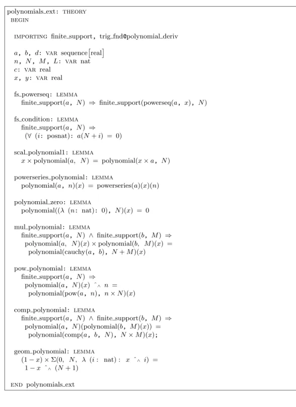
polynomials ext: theory begin
importing finite support, trig fnd@polynomial deriv
a, b, d: var sequence£real¤ n, N , M , L: var nat c: var real
x, y: var real fs powerseq: lemma
finite support(a, N ) ⇒ finite support(powerseq(a, x), N ) fs condition: lemma
finite support(a, N ) ⇒
(∀ (i: posnat): a(N + i) = 0) scal polynomial1: lemma
x × polynomial(a, N ) = polynomial(x × a, N ) powerseries polynomial: lemma
polynomial(a, n)(x) = powerseries(a)(x)(n) polynomial zero: lemma
polynomial((λ (n: nat): 0), N )(x) = 0 mul polynomial: lemma
finite support(a, N ) ∧ finite support(b, M ) ⇒ polynomial(a, N )(x) × polynomial(b, M )(x) =
polynomial(cauchy(a, b), N + M )(x) pow polynomial: lemma
finite support(a, N ) ⇒ polynomial(a, N )(x) ˆ∧ n =
polynomial(pow(a, n), n × N )(x) comp polynomial: lemma
finite support(a, N ) ∧ finite support(b, M ) ⇒ polynomial(a, N )(polynomial(b, M )(x)) =
polynomial(comp(a, b, N ), N × M )(x); geom polynomial: lemma
(1 − x) × Σ(0, N , λ (i : nat) : x ˆ∧ i) =
1 − x ˆ∧ (N + 1)
end polynomials ext
Figure 2: Abridged extensions to the theory on polynomial (see file polynomi-als_ext.pvs)
taylor model£
N : nat, (importing interval@interval) domInterval: Interval¤
: theory begin tm: type = £ #P : fs type, I: Interval#¤ tm equal: axiom t = u ≡
polynomial(t‘P , N ) = polynomial(u‘P , N ) ∧ t‘I = u‘I; t + u : tm: tm = (#P := t‘P + u‘P , I := t‘I + u‘I#); −t: tm = (#P := −t‘P , I := −t‘I#);
c × t: tm = (#P := c × t‘P , I := ££c¤¤×t‘I#)
t × u: tm = (#P := trunc(cauchy(t‘P , u‘P ), N ), I := ... #) inv(t: {t: tm | same condition as below tm_inv_sharp }):
tm = (#P := ... , I := ... #) containment(f : £
domIntervalType → real¤
, t: tm): bool = ∀ xu: (f (xu) − polynomial(t‘P , N )(xu)) ## t‘I tm add sharp: lemma
containment(f , t) ∧ containment(g, u) ⇒ containment(f + g, t + u) tm scal sharp: lemma
containment(f , t) ⇒ containment(x × f , x × t) tm neg sharp: lemma
containment(f , t) ⇒ containment(−f , −t) tm mult sharp: lemma
containment(f , t) ∧ containment(g, u) ⇒ containment(f × g, t × u) tm inv sharp: lemma
∀ (f : £ domIntervalType → nzreal¤ , t: {t: tm | t‘P (0) 6= 0 ∧ (t‘I/intervalFromRealSeq(t‘P , N ))‘lb 6= 0 ∧ (t‘I/intervalFromRealSeq(t‘P , N ))‘ub 6= 0 ∧ (t‘I/intervalFromRealSeq(t‘P , N )) > −1}): (∀ xu: polynomial(t‘P , N )(xu) 6= 0 ∧
(f (xu) − polynomial(t‘P , N )(xu))/polynomial(t‘P , N )(xu) 6= 1 ∧ polynomial(λ (i: nat):
if i = 0 then 0 else −t‘P (i)/t‘P (0) endif, N ) (xu) 6= 1) ∧ Zeroless?(££ t‘P (0)¤¤ ) ∧ Zeroless?( ... ) ∧ Zeroless?(intervalFromRealSeq(t‘P , N )) ∧ containment(f , t) ⇒ containment(1/f , inv(t))
12 Francisco Ch´aves and Marc Daumas
3
Taylor models
Taylor models (Makino and Berz [2003]) are pairs t = (P, I) where P are polyno-mial functions of fixed degree N and I are intervals. N is a constant that cannot be changed during the evaluation of expressions. In PVS, pairs are defined using components between (# and #). Components can be addressed independently using quotes ‘, that are t‘P and t‘I.
Taylor model t is a correct representation of function f if it satisfies the con-tainmentpredicate stated Figure3,
∀x ∈ J f (x) − t0P (x) ∈ t0I
where J is usually [−1, 1].
Our first task was to define operations on Taylor models. Addition, negation and multiplication by a scalar are straight forward and can be read directly from Figure 3. Naive multiplication of Taylor models creates polynomials of degree 2N . The high order terms of the polynomials must be truncated and are accounted for in the interval part.
The inv reciprocal operator uses the following equality where r ∈ I, p(0) 6= 0 and p(x) has the same sign as p(0).
1 p(x) + r = 1 p(0)· p(x) p(x) + r · 1 1 −³1 −p(x)p(0)´ (1) We define q(x) = 1 −p(x)p(0) and we expand the last fraction of (??) using the geomet-rical seriesPN
i=0qi truncated to keep only a polynomial of degree N .
Decorrelation forbids to evaluate the penultimate fraction of (??) directly and we defined a new operator based on the lower bound and the upper bound of I/p(J) that returns directly
1 1 +lb0(I/p(J))1 , 1 1 +ub0(I/p(J))1 .
This operator cannot be replaced by a direct implementation of 1
1 + p(J)/I or
1 1 +I/p(J)1
because I usually contains 0 preventing anyone to use it as a divisor.
We also implemented the exponential of Taylor models using the following equal-ity where r ∈ I and ˆex is a rational approximation of ex.
ep(x)+r = ˆep(0)· ep(x)−p(0)·e
p(0)
ˆ ep(0)· e
r
The polynomial part of the result is obtained by developing and truncating the exponential series composed with p(x) − p(0). The interval part is set accordingly to account for all discarded quantities.
The five _sharp lemmas of the second part of Figure 3, show that the con-tainment predicate is preserved by our operators. It means that we can deduce properties from evaluations of expressions using Taylor models.
In addition to prove mathematical theories, PVS provides a ground evaluator. It is an experimental feature of PVS that enables the animation of functional specifi-cations. To evaluate them, the ground evaluator extracts Common Lisp code and then evaluates the code generated on PVS underlying Common Lisp machine.
Uninterpreted PVS functions can be written in Common Lisp. PVS only trusts Lisp codes generated automatically from PVS functional specifications, then one can not introduce inconsistencies in PVS. However, codes are not type-checked by PVS and can break inadvertently.
PVSio9 is a PVS package developed by Mu˜noz that extends the ground evalua-tor with a predefined library including imperative programming language features. PVSio loads in emacs interface using M-x load-prelude-library PVSio and then executes with M-x pvsio.
4
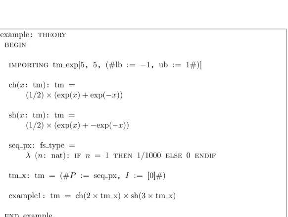
Toy example, concluding remarks and future work
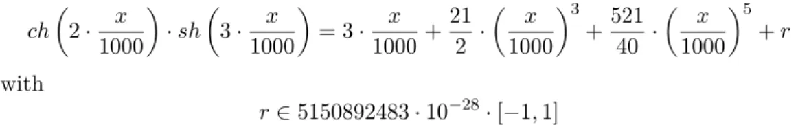
Figure 4 show how easily we can define expressions. PVSio is used to evaluate Taylor model expressions and Figure 5 shows the polynomial and interval parts of the Taylor model of degree 5 of
ch µ 2 · x 1000 ¶ · sh µ 3 · x 1000 ¶ = 3 · x 1000+ 21 2 · µ x 1000 ¶3 +521 40 · µ x 1000 ¶5 + r with r ∈ 5150892483 · 10−28· [−1, 1]
Coefficients are obtained from expressions example1‘P(0), P(1) down to P(5). The interval part is example1‘I.
14 Francisco Ch´aves and Marc Daumas example: theory begin importing tm exp[5, 5, (#lb := −1, ub := 1#)] ch(x: tm): tm = (1/2) × (exp(x) + exp(−x)) sh(x: tm): tm = (1/2) × (exp(x) + −exp(−x)) seq px: fs type =
λ (n: nat): if n = 1 then 1/1000 else 0 endif
tm x: tm = (#P := seq px, I := [[0]]#)
example1: tm = ch(2 × tm x) × sh(3 × tm x)
end example
Figure 4: A toy example of Taylor models (see file example.pvs)
<PVSio> example1‘P(0); ==> 0 <PVSio> example1‘P(1); ==> 3/1000 <PVSio> example1‘P(2); ==> 0 <PVSio> example1‘P(3); ==> 21/2000000000 <PVSio> example1‘P(4); ==> 0 <PVSio> example1‘P(5); ==> 521/40000000000000000 <PVSio> example1‘I; ==> (# lb := -1996666003792920908077809559596469417049924988435 67542489125827927772468257695416279793105352103584647/38763 49604747870233132233643700469577302245603256513727240130672 32422339563866364336668581220000000000000000000000000000, ub := 1996666003792920908077809559596469417049924988435 67542489125827927772468257695416279793105352103584647/38763 49604747870233132233643700469577302245603256513727240130672 32422339563866364336668581220000000000000000000000000000 #)
16 Francisco Ch´aves and Marc Daumas
To conclude, we would like to say that they have three goals in presenting this report:
Present an accurate report of the work involved including the train-ing of a PhD student to PVS. Though this development is significant, PVS validated projects can be achieved in a reasonable time-frame provided appropriate tutoring is available.
Provide a simple tutorial to our library on Taylor models. Readers should be able to start validating their own results as soon as they have finished reading this paper.
Offer a first easy step to the usage of automatic proof checkers. It is always frustrating to spend time on questions than can easily be solved by more or less elaborate techniques. As we now provide a PVS library for interval arithmetic and for Taylor models, one should be able to answer quickly to most of the easy questions about round-off, truncation and modeling errors. Concentrating only on intricate questions is rewarding from the academia and ensures financial support from the industry.
In the future, we will implement more operations on Taylor models like square root, sine, cosine, and arctangent. We will also create PVS strategies to hide more and more details of Taylor models to users. Our main goal remains to help provide invisible formal methods.
Acknowledgements
The authors wish to express all their gratitude to Cesar Mu˜noz from the National Institute of Aerospace in Hampton, Virginia, for his tutoring and help in the many manipulations around PVS. The authors would also like to thank NASA Langley Research Center for its free PVS Class held on May 24-27, 2005.
References
Amir D. Aczel. Fermat’s last theorem: unlocking the secret of an ancient mathemat-ical problem. Four Walls Eight Windows, 1996.
Yves Bertot and Pierre Casteran. Interactive Theorem Proving and Program Devel-opment. Springer-Verlag, 2004.
Marc Daumas, Guillaume Melquiond, and C´esar Mu˜noz. Guaranteed proofs using interval arithmetic. In Paolo Montuschi and Eric Schwarz, editors, Proceedings of the 17th Symposium on Computer Arithmetic, Cape Cod, Massachusetts, 2005. Debbie Gage and John McCormick. We did nothing wrong. Baseline, 1(28):32–58,
2004.
Information Management and Technology Division. Patriot missile defense: software problem led to system failure at Dhahran, Saudi Arabia. Report B-247094, United States General Accounting Office, 1992.
Luc Jaulin, Michel Kieffer, Olivier Didrit, and Eric Walter. Applied interval analysis. Springer, 2001.
Jacques-Louis Lions et al. Ariane 5 flight 501 failure report by the inquiry board. Technical report, European Space Agency, Paris, France, 1996.
Kyoko Makino and Martin Berz. Taylor models and other validated functional inclu-sion methods. International Journal of Pure and Applied Mathematics, 4(4):379– 456, 2003.
Ramon E. Moore. Interval analysis. Prentice Hall, 1966.
Arnold Neumaier. Interval methods for systems of equations. Cambridge University Press, 1990.
Sam Owre, John M. Rushby, and Natarajan Shankar. PVS: a prototype verification system. In Deepak Kapur, editor, 11th International Conference on Automated Deduction, pages 748–752, Saratoga, New-York, 1992. Springer-Verlag.
Sam Owre, Natarajan Shankar, John M. Rushby, and David W. J. Stringer-Calvert. PVS Language Reference. SRI International, 2001. Version 2.4.
Sam Owre, Natarajan Shankar, John M. Rushby, and David W. J. Stringer-Calvert. PVS System Guide. SRI International, 2001. Version 2.4.
Philip E. Ross. The exterminators. IEEE Spectrum, 42(9):36–41, 2005.
John Rushby and Friedrich von Henke. Formal verification of algorithms for critical systems. In Proceedings of the Conference on Software for Critical Systems, pages 1–15, New Orleans, Louisiana, 1991.
18 Francisco Ch´aves and Marc Daumas
Ashish Tiwari, Natarajan Shankar, and John Rushby. Invisible formal methods for embedded control systems. Proceedings of the IEEE, 91(1):29–39, 2003.
Unité de recherche INRIA Futurs : Parc Club Orsay Université - ZAC des Vignes 4, rue Jacques Monod - 91893 ORSAY Cedex (France)
Unité de recherche INRIA Lorraine : LORIA, Technopôle de Nancy-Brabois - Campus scientifique 615, rue du Jardin Botanique - BP 101 - 54602 Villers-lès-Nancy Cedex (France)
Unité de recherche INRIA Rennes : IRISA, Campus universitaire de Beaulieu - 35042 Rennes Cedex (France) Unité de recherche INRIA Rocquencourt : Domaine de Voluceau - Rocquencourt - BP 105 - 78153 Le Chesnay Cedex (France)