Phase transformations and microstructure evolutions in metastable beta titanium alloy Ti-B19

(1)

HAL Id: tel-01749447

https://hal.univ-lorraine.fr/tel-01749447

Submitted on 29 Mar 2018

HAL is a multi-disciplinary open access archive for the deposit and dissemination of sci-entific research documents, whether they are pub-lished or not. The documents may come from teaching and research institutions in France or abroad, or from public or private research centers.

L’archive ouverte pluridisciplinaire HAL, est destinée au dépôt et à la diffusion de documents scientifiques de niveau recherche, publiés ou non, émanant des établissements d’enseignement et de recherche français ou étrangers, des laboratoires publics ou privés.

metastable beta titanium alloy Ti-B19

Hui Chang

To cite this version:

Hui Chang. Phase transformations and microstructure evolutions in metastable beta titanium alloy Ti-B19. Other. Institut National Polytechnique de Lorraine, 2010. English. �NNT : 2010INPL053N�. �tel-01749447�

(2)

AVERTISSEMENT

Ce document est le fruit d'un long travail approuvé par le jury de

soutenance et mis à disposition de l'ensemble de la

communauté universitaire élargie.

Il est soumis à la propriété intellectuelle de l'auteur. Ceci

implique une obligation de citation et de référencement lors de

l’utilisation de ce document.

D'autre part, toute contrefaçon, plagiat, reproduction illicite

encourt une poursuite pénale.

Contact : ddoc-theses-contact@univ-lorraine.fr

LIENS

Code de la Propriété Intellectuelle. articles L 122. 4

Code de la Propriété Intellectuelle. articles L 335.2- L 335.10

http://www.cfcopies.com/V2/leg/leg_droi.php

(3)

(4)

ACKNOWLEDGEMENTS

The present work would have been impossible without the support of the Sino-French Doctoral College Program and the PRA program (MX05-01).

Here, first of all, I would like to express my great gratitude to my supervisors, Prof. Lian ZHOU and Prof. Elisabeth GAUTIER, from the deep of my heart due to their much more attention paid on my whole Ph.D works. It was through their encouragement and understanding that I could continue to finish my works till today. Special thanks also go to Prof. Gautier for her kindly revision of all the documents and the instructive discussions in skype-meeting during the past days in spite of her column sickness. When I was in Nancy for the doctoral work, she gave me a lot of cares not only in the work but also in life. From all the doctoral process, I have learned a lot of intensive knowledge about titanium and titanium alloys even though I have already worked in this field for many years. Thank you very much for all that you have done for me.

My work would not have been possible without the collaboration and assistance from many individuals. I owe lots of love to all of my colleagues and friends in China and France. Prof. Jinshan LI, Prof. Xiangyi XUE, Prof. Rui HU Mr. Yichuan WANG and Dr. Hongchao KOU have given me great support not only from minds but also from actions, especially, allowing me more free time so that I could write the thesis. A special note of thanks also goes to Dr. Fabien Bruneseaux, who helped me to finish the analysis of the X-ray diffraction results to get the correct data. Here, I would like to thank Dr. Benoît Appolaire for the instructive discussion on the phase theory. The thanks should also be given to Madam Martine Tailleur as well as other colleagues in LSG2M Nancy. During writing the thesis, Dr. Bin TANG and

(5)

Guoqiang SHANG as well as Xiangbo DAI also give me helpful support. Thanks for Prof. Weimin BIAN who helps to do the TEM observations.

Finally, I would like to express my deepest gratitude to my mother, farther in law, and mother in law, they give me strong support during those past days wherever I was. Great thanks should also be given to my wife Ms. Liang FENG and my lovely daughter Miss Shuwen CHANG for their unconditional love and encouragement, which makes me possible to finish all the work and I would like to share all of these with them.

(6)

I. INTRODUCTION

I.1.

Brief introduction of titanium alloys

As an important structural and functional family of material, titanium and titanium alloys have been widely used in many fields such as aerospace, chemical industry, biomechanical applications etc due to the low density, high strength, good corrosion resistance as well as high temperature performances [1~6]. Generally, titanium and titanium alloys can be divided into three different classes, such as α, β and α+β according to the phases present at room temperature. With the development of titanium alloys, a more detailed classification has been made with 5 different classes corresponding to α, near α, α+β, metastable β as well as stable β titanium alloys as shown on a pseudo binary phase diagram in Figure 1-1[2, 5, 14].

Figure 1-1 The pseudo binary phase diagram of Ti alloys and different classes of Ti Alloys.

The alloying elements of titanium are classified as α-stabilizers, β-stabilizers and

T emperature α phase α+β phase β phase Ms β Stabilizer Concentration Near α alloy α alloy _α₊_β_alloy Metastable β alloy Stable β alloy

(10)

neutral according to their influence on the β transformation temperature (T_β). The

α-stabilizers addition stabilizes the α phase and increases the β transformation

temperature, while the β-stabilizers stabilize the β phase and decrease the β

transformation temperature[2,5,6]

. Table1-1 shows the alloying elements and their function in titanium alloys.

Table 1-1 Classification and effect of alloying elements in Titanium alloys [4]

In order to compare the alloys, and the relationships between the chemical composition, the phases present and the mechanical properties in titanium alloys, the

aluminum-equivalent (expressed as [Al]Eq.) and molybdenum-equivalent (expressed

as [Mo]Eq.) have been used to describe the stability and strengthen ability of an alloy [1~4, 6]

, and can be calculated with the following formulations:

Alloying elements category Phase diagram

Interstitial elements Main elements α-stabilizers Beta Alpha+Beta Alpha 882C T X(% massive) O,N,B,C Al β-stabilizers Isomorphous elements T 882C Alpha Alpha+Beta Beta X(%) Mo, V, Nb, Ta Eutectic elements Alpha Alpha+Beta Beta Beta+TiX Alpha+TiX T 882C H Mn, Fe, Cr, Co,

W, Ni,Cu, Au, Ag,

Si Neutral Beta Alpha+Beta Alpha T 882C X(%) Sn, Zr

(11)

% 10 % 6 / 1 % 3 / 1 % [Al]_Eq = Al + Sn + Zr + O₂

[ ]

Mo Eq.=Mo% 1 1.5 % 1 0.6+ V + Cr% 1 0.35+ Fe% 1 1.3+ Cu% 1 3.6+ Nb%

By now, more than 100 different titanium alloys are known, in which only 20~30 alloys have been used as commercial alloys [3, 5, 6, 15]. According to the performances, different kinds of alloys have been developed for different application fields. For the

α and near α alloys, the microstructure at room temperature is mainly composed of

only α phase or a mixture of α+β phases with very low β phase amount (normally not exceeding 15%). Those kinds of alloys can be used for high temperature parts due to its combination of suitable strength, good weldability, good creep properties as well as thermal stability, such as IMI834 alloy [3, 15]. Meanwhile, some of those alloys can be used in the lower temperature ranges for their nice low temperature properties, for example Ti-5Al-2.5Sn [6]. The α+β class alloy contains α phase and β

phase at room temperature, and normally the α phase volume fraction exceeds 50%,

and the alloys are one of the structural material with excellent mechanical properties. This class can be strengthened by heat treatment and even the strength can be adjusted through the heat treatment. Ti-6Al-4V is a typical α+ß alloy which has been developed in the 1950s [6,15~26], and now it is most widely used, as a structural material. Metastable and stable β titanium alloys contain more β stabilizer elements. For metastable titanium alloys, the amount of ß stabilizer is sufficient to avoid any diffusive or displacive (martensitic) transformation during quenching. The martensitic transformation temperature is lower than the room temperature, and the high temperature ß phase can be remained at room temperature by quenching from solution temperature. Such kinds of alloys have good cold deformability, and can be strengthened by heat treatment by precipitation of α phase from metastable β phase. So these alloys can be used for high strength structural parts, such as Ti-1023 alloy[10,12,13,27~29].

(12)

I.2.

Phase transformation in titanium alloys

I.2.1. Main phase transformations in titanium alloys

As for other metallic alloys [30~34], different solid/solid phase transformations may occur during the thermal treatments in titanium alloy controlling the microstructure and in consequence the properties of the alloy. The study of the solid phase transformations during heat treatments have thus been a necessary research field for the material scientists [29, 34, 35]. In titanium alloy, the basic phase transformation is theα ↔β transformation. The crystal structures of α and β phases are shown in

Figure 1-2 a and b, respectively. The α phase has a hexagonal close packed (HCP)

lattice structure; there are two atoms in each cell with 12 near neighbor atoms.

(a) lattice structure of α-Ti (hcp) (b) lattice structure of β-Ti (bcc) Figure 1-2 Crystal structure of α-Ti (a) and β-Ti (b).

The lattice parameters of α are a= b=2.95Å and c= 4.68Å, giving the c/a ratio of 1.587, that is a little smaller than that of the ideal HCP lattice (c/a=1.633). The β phase has a body-centered cubic (BCC) structure and there are also 2 atoms in each

cell, surrounded by 8 near neighbor atoms. The lattice parameter of bcc β phase is

a=b=c=3.206Å. In titanium alloys, the solid phase transformations can be classified into different kinds and Tingjie Zhang has summarized it as show in Table 1-2 [30].

(13)

Table 1-2 The main phase transformations in titanium alloys

Phase transformation Transformation processing

1 Decomposition of β phase during cooling 1) β →α +β_remains_. 2) Martensite: β→ ′ α + ′ ′ α 3) β →ω_an₋_iso +β_remains 2 Decomposition of ß phase during isothermal processing

1) β_metastable →α +β_remain, β_remains→α +β_transforme_d 2) β β

(

+α

)

→ ′ ′ α (α ′ ′ _rich+ ′ ′ α _poor), β′, βrich, βpoor, 1α, 2α

3) β →ω_iso+β_transforme_d

4) β_remains→β_remains+β_transformed 5) β_remains →α₂+β

6) Isothermal martensite transformation

3

α phase formed via transition phases d transforme remains Metastab ω α β β / → → + , d transforme remains Metastab β α β β / → ′→ + 4 Decomposition of martensite 1) α′→α +β_transforme_d,α′→α +compounds 2) α″( Ms>>Troom) →α +β_transforme_d, α″( Ms≤Troom) →βtransformed 5 Eutectoid decomposition

1) Active eutectoid: pearlite type microstructure 2) No-active eutectoid: mass type microstructure

6

Decompose of α solid solution

Compounds, ordered α2 phase

7 Interface phase α/β interface phase forming at a lower cooling rate.

All these transformations are not observed in all titanium alloys. As the research is mainly focused on β-metastable alloys, the transformations occurring in those alloys will be detailed in the following. At first we will detail the transformations occurring at the lower temperatures.

(14)

I.2.2. Martensitic phase transformation

Martensitic phase transformation is an important solid phase transformation in titanium alloys; it is a first order, non diffusive phase transformation, and the growth is controlled by the movement of the interface. The martensitic phase transformation has an important influence on the mechanical properties and it results in complex microstructure changes. Thus more and more researchers have paid more attention in this field [2, 5, 6, 30, 34, 36~48].

Martensitic phase transformation in titanium alloy can be classified into three different types according to its formation conditions, which includes quenching martensite, isothermal martensite as well as stress induced martensite[30, 34, 48]. Quenching martensite is formed during the cooling from high temperature with an enough quick cooling rate avoiding diffusion of solute elements, isothermal martensite is formed during an isothermal period. Stress induced martensite may be formed for example during tensile tests of a metastable beta phase; martensitic transformation is assisted by stresses including outside loading stress as well as internal stress.

According to the crystal structure, martensite can be classified into four different types[30]: they are {334} hexagonal martensite, {344} hexagonal martensite, orthorhombic martensite as well as FCC martensite. But anyway, the hexagonal Martensite (α′) and orthorhombic martensite (α′′) are familiar in industrial titanium alloys. Normally, α′ martensite exists in the alloys that contain the lower amounts of alloying elements; its crystal structure is HCP. The martensite morphology is plate shaped without internal twins and with a habit plane of

{ }

334 _β, meanwhile the

orientation relationships with the β matrix is:

( ) ( )

111_M //110 _β, 1120 //

[ ]

111_β M     − .

The orthorhombic martensite α′′, is observed in the alloys with higher amounts of alloying elements. Their morphology is needle-like. In those morphologies, there are

(15)

possible internal twins, and the orientation relationships with the β matrix is:

( ) ( )

111M //110 β,

[ ] [ ]

110 M //111β. During further heat treatments, the martensite will

decompose into stable α phase due to its metastable state. The α′ martensite

decomposes directly into stable α phase. However, for α′′ martensite, the

decomposition process is a little more complex; the α′ martensite will be formed first followed by the stable α phase.

The martensite formation conditions in titanium alloy are dependent on the alloy chemical composition (the category and amount of alloying elements) as well as the heat treatment conditions, especially the cooling rate when the alloy is cooled from the high temperature. The influence of the elements position in the periodic table on the martensitic transformation temperature (Ms) have been investigated by A.V. Dobromyslov et al.[40] using more than 150 different binary titanium alloys which content different amount of alloying elements such as V? Cr? Mn? Fe? Co? Ni? Cu? Nb? Mo? Ru? Rh? Pd? Ta? W? Re? Os? Ir? Pt etc.. The results indicated that the alloying elements above mentioned should be added within the critical lowest amounts in order to retain the metastable phase during quenching from high temperature. For the binary alloys for which the added elements have a BCC crystal structure, the Ms point of the alloy will be greatly elevated, and the Ms point increased with the family position of the added element increase in the element periodic table. When the crystal structure of the added elements is FCC, the Ms point of the alloy will be elevated with the family position of the added element decrease in element periodic table.

The research results of Ti-35Nb-7Zr-5Ta alloy by J.I. Qazi et al. [41] shows that α′′ phase forming conditions are nearly related with the alloy chemical composition as

well as the cooling rate. The α′′ phase will be formed in the alloy at the water

(16)

the volume fraction of α′′ phase decreased with the addition amount of Nb+Ta

increase, and the formation of α′′ phase will be inhibited completely when the

addition amount of Zr element is between 4.1~ 4.6%. However the addition of the interstitial elements will counteract such effects of Zr addition.

The results of research on the kinetics of martensite formation in Ti-6Al-4V alloy containing hydrogen reveal that the Ms point of the alloy will be decreased with the

addition of hydrogen[41], and the Ms point will be lower than 500oC when the

additional amount of hydrogen is 30at%. It is also shown that the volume fraction of

α′′ formed during quenching changes from 0% to 80% when the hydrogen addition

amount change from 0at% to 30at%, and the temperature “nose” for the martensitic

transformation decreased from 800oC to 625oC during the following aging treatment

processing. In another point, the starting time of α′′ martensite decomposition is lagged from 6 seconds to 10 minutes when 10at% hydrogen is added in the alloy.

I.2.3. ω Phase transformation

The ω phase is a transition phase in titanium alloy, and often appears in the

metastable beta titanium alloys that contain high amounts of beta stabilizing elements. Two different sorts of ω phase are reported in the literature, one is the quenching or an-isothermal ω phase, and the other one is the isothermal ω phase.

The forming mechanism of an-isothermal ω phase can well be explained by the

theory model of {111}β plane collapse[31,39,49~53]. It is said that the crystal lattice of ω phase is formed by one {111}β plane in the β matrix that collapses to the middle and while the neighbor {111}β planes keeps the original position. The isothermal ω phase is formed during isothermal treatment at low temperatures (300-350°C) and is controlled by diffusion.

(17)

for the detailed crystal structure, there are three different comments. Some researchers consider it is BCC structure[31], and some of them think it is a HCP structure[31]. There are also some authors that take it for a “triangle” structure which is a kind of aberrant HCP structure and normally appears in the alloy which contain high volume fraction of alloying elements[31]. By now, most researchers are apt to

consider the crystal structure as HCP[49~55]. The two kinds of ω phase show

differences in the diffraction patterns, and there are dispersion stripes appearing for an-isothermal ω phase, but not for the isothermal ω phase.

Normally, an-isothermal ω phase shows particle-like shape[27,34,49], and precipitates are dispersed in the β matrix. For the isothermal ω phase, the shape of the precipitates is ellipsoidalwith a size of a few nanometers. Precipitates are dispersed in the β matrix. Moreover, an ω phase with lamellar-liked shape has been reported by Japanese researchers when investigating martensite transformation during

quenching in shape memory alloy of Ti-30Nb-3Pd(wt%)[35]. The crystal structure of

this ω phase is HCP and the precipitate size is of a few nanometers. The orientation relationships between the lamellar-liked ω phase and the β matrix is the same as for the particle-like ω phase. The different morphologies of the ω phase are shown in Figure 1-3a,b[43,46].

Figure 1-3 Dark field TEM image of ϖ phase for ellipsoidal-shaped (a) and lamellar-shaped (b).

D.H. Ping[35] et al., have related the formation mechanism of lamellar-liked ω phase.

(18)

The interface of the lamellar-liked ω phase and β matrix are very plain observed in

the experiment, and the habit plane is close to {112}_β crystal plane where phase

transformed due to shear stress occurred along( 111) crystal orientation.

The ω phase is a transition phase and is not stable, so it will disappear or transform when the alloy is reheated at higher temperatures. The role of the ω phase on the formation of the α phase has been studied in detail [49,51]. In the different studies, the authors have reported that the ω phase favors the nucleation of the α phase. Three different explanations have been proposed. At first [51], it has been proposed that α phase nucleates in the β matrix, at some distance from the ω/β interface, enriched in Al. For other authors [51] the α phase nucleates at the ω / β interface, and grows in β and ω phases consuming the ω phase. During this period, the three different phases

keep the orientation relationship as: ( 1100 )ω//( 1010 )α//( 211 )β,

(1120 )ω//(0001)α//(011) β, (0001)ω//(1210 )α//(111)β. At last, Prima et al[46] have

proposed that α nucleates in the ω phase keeping the following orientation

relationships: (210 )_ω//(002)α, [001]ω//[110]α. Their schematic model is shown in Figure 1-4.

Figure 1-4 Nucleation and growth model of α phase in inner ω phase [46]

.

(a) ω phase act as nuclear site for α phase;(b) α growth in inner ω phase by consuming ω phase; (c) ω phase disappear; (d) α phase growth with the β phase exhaust.

(19)

Anyway, the detail about isothermal ω phase formation mechanisms and phase transformation kinetics is still in research and related experimental data as well as models are still lacking. Uniform answers are not yet obtained. Nevertheless, in order to gain a fine and dispersed distribution of α phase, the processing route with a

low aging temperature leading to ω precipitation followed by high temperature

treatment leading to α formation has been used to reduce the size of α precipitates.

I.2.4. Decomposition of metastable β phase

Depending on the chemical composition of the alloys, the decomposition of the β

phase may occur during the cooling from the high temperature β phase range, or for

β-metastable alloys during reheating processes after high temperature solution

treatment as well as during isothermal aging treatments. Different authors have paid

attention to the formation of α phase during isothermal aging to understand its

mechanism of nucleation and growth, and the related kinetics and crystallography of the phases. Some progresses focused on those aspects will be presented considering at first the transformation on heating and further aging of mainly beta metastable alloys, and in a second part the transformation on cooling of different titanium alloys.

Transformation on heating and aging of beta metastable alloys.

The decomposition of the β phase on aging can lead to the formation of different phases: β′, ω, martensite as well as α. β′, ω, and martensite are not stable phases,

and they will further decompose or transform into stable α phase during the

following thermal process[5,32,56~84]. The transformation of β′ and α phases will be

introduced in detail. Martensite and ω phase transformation have been introduced

above.

(20)

temperature(200~500°C) in titanium alloy which is rich in β stabilizer elements (such as Ti-15-3 ) [51,65]. The β′ phase has the same crystal structure as the parent

phase, and also takes coherent structure with the β phase, but has a lower

concentration of alloying elements as compared with the parent phase. The morphology of β′ phase is very fine (several nanometers) and with short bar-shape or crescent-shape. The stability and transformation kinetics of β′ phase are strongly dependent on the chemical composition of the alloy, and it will be decomposed with

the aging time prolongation until the stable α phase formed. It is very hard to

distinguish the β′ phase and β phase by the X-ray diffraction technology because the difference in lattice parameter is very little, so the film TEM technology should be used to observe the precipitated β′ phase in titanium alloy.

For the direct formation of α phase from the metastable β phase during isothermal aging, the transformation mechanisms, precipitates distributions, volume fraction, appearance as well as the transforming kinetics are strongly influenced by the chemical composition of the alloy, the transformation temperature, the grain size of the parent β phase and the heating rate to the aging temperature[64,65,79,82].

The isothermal phase transformation in Ti-15-3 alloy has been investigated in detail

by Guiqin SHEN[51]. The results related that, when aging at 700°C for 4 hours (the

heating rate to 700°C is not reported), the α phase is first formed at grain boundaries. After 12 hours holding at 700°C, intragranular α precipitates are observed and the transformation is completed after nearly 48 hours. The final α volume fraction is

about 22%. Decreasing the aging temperature, the β→α transformation kinetics is

accelerated. At 600oC, the α phase begins to precipitate after 15 minutes holding, and is finished after 24 hours holding, and the final volume fraction of α phase is

about 41%. Meanwhile, at 550 and 500°C, the beginning of the transformation is

(21)

finished after 12 hours. The volume fractions of α phase are 50% and 62% (measured by X-ray diffraction), respectively. TEM observations have been performed for a Ti-15-3 alloy by Furuhara[79]. The observations revealed that the α phase formed during aging at temperatures above 450oC (Figure 1-5) has a lath morphology. For an aging temperature of 300oC (3600s), α is present and has an aggregated morphology, composed with thin twinned laths (Figure 1-5).

Figure 1-5 Variations of α phase morphology and crystallography with aging temperature in Ti-15-3 [79].

Different studies report the existence of alpha phases presenting two different orientation relationships. THOMAS J. et al.[31] have observed these two different

kinds of α phase formed in Ti-38644 alloy during aging treatment at 350oC~400oC

and above 450°C, respectively, named 1α and 2α. The orientation relationships between 1α and β are the Burgers one, i.e.:

{ }

110 // 0001 ; 111 // 1120

{ }

_α

[ ]

_β

α

β   1α

morphology is lens-liked and is twinned with a habit plane of

{ }

0111 . 2α and the matrix do not obey to the Burgers orientation relationships; the morphology of 2α shows raft-liked shape. 2α presents also a twinned structure and the twin plane is the same as for 1α phase. C.G. Rhodes and J.C. Williams[47] considered that there are no difference in crystal structure between the two kinds of α phase, but the 2α is more

stable than 1α and during its growth it consumes 1α. Moreover, they proposed that

there are two possible different mechanisms for the formation of 2α: one mechanism

(22)

formation of 2α by nucleation and growth. R. Jeffrey et al[24] have also reported the formation of 1α and 2α in Ti-10-2-3 alloy. 1α has been observed in the alloy during aging at temperature above 550oC, while for aging at temperature lower than 550oC, 1α phase and 2α can be observed after decomposition of β.

Isothermal Transformation during cooling from the high β temperature range.

Characterizations of transformation have also been performed during isothermal treatments after direct cooling from the stable beta temperature range. Studying metastable alloys such as βCEZ or Ti17 [80~82] three different morphologies of α phase have been identified depending on their nucleation sites, and the condition of transformation. The first called αGB morphology is formed at first at the β grain boundaries; the second one defined as αWGB morphology grows from αGB and is observed as colonies of lamellae with a same crystallographic orientation [80]. The last one called αWI or αWM precipitates in the β grains and present a Widmanstätten

morphology; the precipitates arrangement look as a basketweave. For βCEZ and Ti17,

the results indicate that αGB and αWGB are mainly formed at temperatures above 750°C; the average width of αGB is about 2.3µm, the maximal length of αWGB phase is about 40µm[109]; when the isothermal temperature is 700oC, the three kinds of morphologies are observed, that is to say αGB, αWGB and αWI phase. At that transformation temperature, the average width of αGB phase is about 1.3µm, the length of αWGB phase is less than 0.5µm; when the isothermal temperature is 600oC, and the average width of αGB is about 0.2µm.

The authors also consider that the β phase between the αWGB lamellae is enriched in

β stabilizer elements, while its chemical composition ahead of the lamellae tip is modified on a shorter distance. The length of the αWGB lamellae is decreased with the

decrease of the transformation temperature for example, it is 10~20µm when the

(23)

750oC. A numerical model describing the formation sequences of the α phase at high isothermal temperatures has been proposed according to the experimental observations, and has been schematized as the sequence shown in Figure 1-6.

Figure 1-6 Sequence of the phase transformation modeling established based on βCEZ alloy at high

temperature isothermal treatment [101].

(a) nucleation of αGB, (b) growth of αGB, (c) appearance of αWGB, (d) growth of αWGB.

Studies performed by S.Malinov et al[84,85] on Ti-6-4, Ti-811 and Ti-6242 alloys have led to similar observations but at different temperature ranges. Above 900oC the α phase is first formed at the β grain boundaries and the lamellar α phase nucleates and grows in the β grain; at lower temperatures, lamellar α grains nucleate and grow uniformly in the β grains.

I.3.

The phase transformation kinetics of titanium alloys

The solid phase transformation kinetics in alloys can be established by a continuous characterization of changes of physical properties which are sensitive to the structural evolutions leading to a relationship of the relative change of property with temperature and time[86~90]. These properties can be expansion coefficient, volume, hardness, electrical resistivity as well as enthalpy changes etc.. Assuming a linear relationship between those relative properties and the relative structural change, the

(24)

equation between the phase transforming degree (f) and those changes of physical parameters can be given as:

0 1 0 p p p p f − − = , 0≤ f ≤1 ( 1-1)

where, P is the value of the measured physical parameters at time t; P1 and P0 are the values of the measured physical parameters at the beginning and at the end of the phase transformation, respectively.

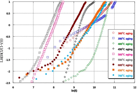
The isothermal kinetics of the transformation will be expressed as f = f(t). For diffusive transformations, the transformation kinetics often presents a sigmoid shape that is expressed by JMAK law (Equation 1-2).

(

( )

)

) exp 1 ( max 0 1 0 n b t t k f p p p p f = − − − − − = ( 1-2)

Here, k means the temperature coefficient which is sensitive to the variation of temperature; n is the Avrami exponent; t is time at transformation temperature and tb is the beginning time for the transformation. The Avrami coefficient is dependant on the nucleation and growth mechanisms.

In order to model the transformation during cooling, different models have been established. Considering additive characters for both the incubation time and the progress of the transformation, the an-isothermal processing can be treated as series of different very short isothermal steps [91,95]. The beginning of the transformation will be calculated according to Scheil law:

dt t_b

( )

T =1

0

t

(25)

Here, tb(T) is the time at which transformations begins at the isothermal temperature T, and t is the time. The JMAK equation can be expressed as formula 1-4 for the

an-isothermal processing: 1 / 0 0 1 ( ) 1 exp ( ) ln( ) 1 m t m f t k T dt f  _ _    = − _−_ + _ _ −     

∫

 _{( 1-4)}

Here, f0 is the volume fraction of new formed phase at the phase transformation start,

and m is the Avrami exponent for an-isothermal treatment.

Then the relationship between phase transformation degree and time or temperature can be calculated for the isothermal and an-isothermal processing according to JMAK law based on the experimental results. Generally, the an-isothermal phase transformation kinetics can be investigated and calculated based on the research or calculated results of isothermal ones [4, 91~95]. For the titanium alloy, research and calculation on the phase transformation kinetics in Beta CEZ, Ti-17, Ti-6-4, Ti-6242, Ti-811, Ti-1023 as well as Beta21s have been done by E. Laude, J. Da Costa Teixeira and S. Malinov etc. [84,85,91,102,109], and the research results indicated that the JMAK equation can be used to describe the isothermal phase transformation kinetics in titanium alloy.

I.4.

The aim of the present research work

Excellent combination of mechanical properties can be obtained in titanium alloys by controlling the heat treatment process. So it is very important to understand in detail the phase transformations occurring during the process in order to improve the mechanical properties by controlling the microstructure formation and design the deformation and heat treatment. Anyway, it is also an important guide to design and

(26)

develop new alloys.

Ti-B19 is a kind of new metastable beta titanium alloy developed by China. Remarkable combination of mechanical properties as strength, ductility and toughness can be obtained by appropriate heat treatments. The microstructure of the alloy is strongly depended on the parameters of the heat treatment, that is to say the difference of temperature, time and the rate of heating and cooling will lead to differences in volume fraction, shape, size as well as distribution of the formed phase, which introduce differences in mechanical properties. So the aim of the present work is to study the phase transformation kinetics in Ti-B19 alloy during heating and cooling as well as isothermal periods, and to understand the phase transformation behaviors. The results of this work will provide some important data to understand the microstructure evolution as well as some guides to design the processing route (deformation and heat treatment) for a new composition of titanium alloys.

(27)

II. RESEARCH SCHEME AND

EXPERIMENTAL PROCEDURE

II.1.

Research contents

The phase transformation kinetics during isothermal and an-isothermal processing (continuous cooling) in the metastable beta titanium alloy Ti-B19 have been investigated systematically considering the influence of several processing parameters. The nature of the formed phase is analyzed as well as the microstructure evolutions. According to the results, the TTT diagram has been determined for the Ti-B19 titanium alloy for transformation of beta metastable phase during aging. Additional results have been obtained for precipitation during cooling allowing establishing a part of the CCT diagram. These results are a basic work for establishing the relationships between mechanical properties, heat treatment and microstructure. All the work was performed on TiB19 alloy. Our research focused on the following points:

( 1) The isothermal phase transformation kinetics during aging for temperatures in the range of 300~700oC.

( 2) The structure and microstructure evolutions for the given temperatures. ( 3) The influence of heating rate on the phase transformation kinetics and

microstructure evolutions.

( 4) The an-isothermal phase transformation kinetics and microstructure evolution during continuous cooling from the beta temperature range. ( 5) The influence of plastic deformation on isothermal phase transformation

kinetics and microstructure evolution during aging.

( 6) The relationships between mechanical properties, microstructure evolution and heat treatment.

(28)

II.2.

Researching routes

The researching routes of the present work are designed as Fig.2-1. Firstly, in-situ electrical resistivity measurements have been used to get the relationships between kinetics of resistivity variations and treatment temperature, time and processing parameters. Then the phase transformation kinetics has been analyzed, considering a global modeling approach as the JMAK law, and the TTT diagram has been designed. Meanwhile, the nature of the phases, the nucleation and growth of the phases as well as microstructure evolutions have been investigated through synchrotron high energy X-ray diffraction, optical microscopy (OM), electron microscopy (SEM and TEM). Finally, the relationships between mechanical properties, aging temperature and microstructure parameters have been analyzed.

Figure 2-1 Scheme for research route of the present works

The phase transformation kinetics and microstructure evolutions in Ti-B19 alloy

Isothermal processing An-isothermal

processing Relationships of resistivity-temperature-time Phase transformation kinetics Analysis of the phases formed Microstructure observation

α Phase nucleation Microstructure evolution TTT Diagram CCT Diagram Relationships of resistivity-temperature-time Phase transformation Kinetics Microstructure observation Microstructure evolution Mechanical properties Relationship of properties-phase transformation-microstructure

(29)

Based on the designed research routes and results, the research plan of isothermal kinetics, influence of heating rate and plastic deformation on isothermal phase transformation kinetics and phase transformation process during continuous cooling have been designed and described as following, respectively.

II.2.1. Study of isothermal phase transformation kinetics

In order to investigate systematically the isothermal decomposition of β metastable

phase in Ti-B19 alloy a wide range of temperature has been selected. The temperature is ranging from 300oC to 700oC. The holding time at the transformation temperature is varying, depending on the end of the transformation time. The treatment applied to the specimens is schematized in Figure 2-2. For all specimens, a first solution treatment in the β temperature range is realized to control the initial state and the β grain size. The heating rate is 5°C/s, the temperature is 900oC, with

10 minutes holding time and a cooling rate of 20oC/s is used to freeze the

microstructure obtained after the solution treatment at high temperature and keep a metastable β state.

Figure 2-2 Program for isothermal phase transformation behaviors investigation

700? 650? 600? 550? 500? 450? 400? 350? 300? T _β T t 900? ,10 min 5 ? /s >20? /s 10? /s >20? /s

(30)

As transformation kinetics is obtained during aging, and in order to avoid or limit

any transformation on heating before the isothermal decomposition of the β phase, a

heating rate of 10°C/s has been applied.

After isothermal transformation during the aging treatment, specimens have been quenched at a rate higher than 20°C/s, avoiding thus a further precipitation and allowing freezing the microstructure obtained after transformation during aging. The microstructure observations and synchrotron X-ray diffraction analysis have been performed after those treatments. In order to analyze the isothermal phase transformation sequences, samples have been quenched at different holding time

during isothermal treatment at 400oC, 500oC, and 600oC, according to the

transformation kinetics obtained by electrical resistivity. For the sample transformed

at 400oC, specimens have been quenched after 11,000s and 21,000s, holding time;

for the sample treated at 500oC, the holding times have been 1,000s and 2,000s;

while for the sample treated at 600oC, the holding times have been 2,500s, 6,000s

and 10,800s.

II.2.2. Study of the influence of heating on isothermal phase transformation

Heating rate may influence the isothermal phase transformation kinetics and microstructure evolution remarkably. So the influence of heating rate on isothermal phase transformation behaviors have been studied as schematically shown in Fig.2-3. The first solution treatment in the beta temperature range is the same as previously leading to a similar beta metastable state. A single aging temperature is selected as 500oC and the holding time for all conditions is four hours. Three heating rates have been applied 10oC/s, 1oC/s and 0.1oC/s, respectively. After transformation, a rapid cooling rate is applied to freeze the microstructure formed during aging. The cooling rate was more than 20oC/s.

(31)

samples were quenched from 350oC, 450oC and 500oC, respectively, in order to analyze the structure and microstructure evolutions.

Figure 2-3 Applied treatments to study the influence of heating rate on

the isothermal phase transformation

II.2.3. Study of the phase transformation kinetics during continuous cooling.

For the previous conditions, we applied a cooling rate from the beta temperature range leading to a beta metastable state. However, during cooling processes phase transformation may occur depending on the local cooling rate in the material. So the phase transformation kinetics and microstructure evolutions have been studied in

Ti-B19 alloy during cooling from 900oC to room temperature according to the

programs showed in Fig.2-4. The solution temperature of all samples are 900oC and

holding time was 10 minutes with a heating rate of 5oC/s. The cooling rates

considered were the following: 1oC/s, 0.2oC/s, 0.1oC/s, 0.06oC/s and 0.03oC/s, respectively. 500 ? T_β T 900 ? ,10 min 10o C/s 1o_C/s _0.1o C/s t 5 ? /s > 20 ? /s > 20 ? /s

(32)

II.2.4. Influence of plastic deformation of the beta metastable phase on isothermal phase transformation kinetics during aging.

At last, we analyzed the influence of plastic deformation of the beta metastable phase on isothermal phase transformation during aging. The aging temperature considered was 500°C. Two levels or pre deformation of 43% and 52% were considered.

Figure 2-4 Applied cooling rates to study the phase transformation during continuous cooling.

II.3.

Experimental materials

II.3.1. Brief introduction of Ti-B19 alloy

Ti-B19 is a metastable beta titanium alloy developed by China, with a good combination of properties: high strength, high toughness and reasonable ductility as well as a good stress corrosion resistance [102]. The nominal chemical composition of Ti-B19 is Ti-3Al-5Mo-5V-4Cr-2Zr (wt%), and the typical physical properties are listed in Table 2-1. The T_β temperature is 790°C.

Previous studies have shown that [103] Ti-B19 alloy is a kind of alloy which integrates the α/β Ti alloys and β Ti alloys. The molybdenum equivalent of the alloy is

[Mo]eq=15 and the alloy presents enhanced heat treatments capacities. Ti-B19 alloy

1? /s 0.2? /s 0.1? /s 0.06? /s 0.03? /s T t T_β 5? /s 900? ,10min.

(33)

forging can be realized in the β and metastable β temperature range, and further

aging treatments in the α+β range may lead to tensile strength higher than 1250MPa;

the elongation can be maintained at a level higher than 6% with K1C higher than

70MPa⋅m1/2; more favorable matching among strength-plasticity-tenacity can be

gained in metastable alloy.

Table 2-1: Some physical properties of Ti-B19 alloy

Phase transformation point(oC) Density g/cm3 Thermal expansion coefficient ×10-6·? Coefficient of thermal conductivity W/m.k Thermal diffusion coefficient ×10-6m2/s 790±5 4.77 8.2~8.9 (100~300? ) 6.9~11.8 (25~300? ) 2.78~4.09 (25~300? )

II.3.2. Preparation of materials and samples

The Ti-B19 alloy used for this thesis comes from finely forged bars sized in Φ20mm.

The alloy is obtained by a triple VAR process. The preparation and manufacturing processes are the following: sponge-structured Ti and master alloy are combined according to the nominal composition of the alloy and prepared to make an electrode;

then, the material is made into ingot (Φ296mm) through Vacuum Arc Remelting

process. The chemical composition of the alloy is given in Table 2-2.

Table 2-2 Chemical composition of Ti-B19 alloy used in present work. (wt.%)

Elements Al Mo V Cr Zr C N H O Fe Si Ti

Content 3.3 4.7 5.1 4.0 1.92 0.01 0.08 0.01 0.01 0.08 <0.04 Balance

The ingot is further forged in the β-phase range to breakdown the solidification

microstructure and it size is reduced to a forged billet of 60mm in diameter; finally, the billet is transformed into bars of 20 mm diameter on KF-16 precision forger.

(34)

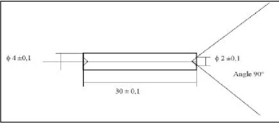
Cylindrical samples, 4 mm in diameter and 30 mm length as shown in Figure 2-5, are machined from the bar by linear cutting. No heat treatment has been done on the specimens.

The β transus temperature of the Ti-B19 alloy is 760±5oC. This value has been

obtained by metallographic observations as well as by differential thermal analysis. The wrought microstructure of the alloy is typical of a deformed microstructure, as shown in Figure 2-6. A certain amount of α-phase is present.

Figure 2-5 Size of the Ti-B19 alloy sample used in the present work (mm)

Figure 2-6 The microstructure of Ti-B19 alloy after forging 100 µm 100 µm

(35)

II.4.

Experiment methods and devices

II.4.1. In-situ resistivity measurement method and device

The tests have been performed at LSG2M (Institut National Polytechnique de Lorraine Nancy) on an in house dilatometer able to characterize simultaneously the electrical resistivity changes.

The phase transformation kinetics is analyzed thanks to electrical resistivity measurements. The basic principle of the resistivity measurement is as follows: during phase transformations in the alloy different changes will occur (variations in the lattice structure, nature, density of interfaces, differences in chemical compositions of the phases) resulting in changes in the electrical resistivity [84,101]. Therefore, it is possible to determine the dynamical changes by measuring the variation of the resistivity of the material in the thermal-mechanical process, so as to determine the kinetics of the structure evolutions.

Figure 2-7 is the diagram of the resistivity measurement method used. The samples

used are usually cylindrical shape sized (diameter of Φ3~4mm and the length of

30~40mm); moreover, sheet-shaped samples are also often utilized in the dimensions of (0.5~0.8) × (3~4) × (20~30) mm. To reach changes in electrical resistivity, the most frequent way is to apply constant current on the sample and to measure the voltage variations. The calculation formula for the resistivity ρ is as follows:

ρ=( )U / I ×( )A L (2-1) Wherein, A is the sectional area (m2) of the sample; L is the distance (m) between the two voltage measurement points; I is the loading current (A), which is a constant value; U is the voltage (V) measured during the experiment.

(36)

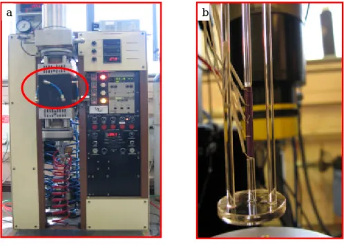
treatment process as a function of time. A further analysis of the obtained data will lead to a dynamical description of the phase transformation kinetics. Test equipment is shown in Figure 2-8. The system mainly includes the following parts:

? A sample heating chamber. This unit is connected with a vacuum system and the dynamic vacuum is as high as 10-5Pa.

? A heating furnace. This unit comprises four infra-red lamps mounted inside the heating chamber. The power applied to the lamps is computer controlled; the

heating rates may vary in the range 0.001~100oC/s; the temperature difference

between interior and exterior of the sample is ±2oC.

? A sample cooling system. It utilizes a computer to control the flow rate of inert gas, so as to control the cooling rate (0.001~150oC/s) of the sample.

? An acquisition and treatment system for the experimental data. It includes sample temperature measurements using thermocouples (Pt/Pt-10%Rh), resistivity variation data acquisition (platinum wire), computer hardware and software for all system control and data process. An electronic treatment is realized to amplify (9000x) the electrical tension variations in order to gain in sensitivity.

Figure 2-7 The schematic diagram of resistivity measurements for phase transformation

To lower oxidation of the sample during the heat treatment, the sample chamber

? ? ? ? ? ? ? ? ? - ? ? ? ? ? ? ? Sa m p l e S a mp l e Computer Control Center

(37)

should be under vacuum during the whole process.

For our experiments, the current applied to the sample is constant, with a value of 2A supplied by an external battery; the connection wires are made of Pt with a diameter of 0.4mm. The voltage variation of the sample during the treatment is measured with two Pt wires (or Pt/Rt-Rh) 0.2mm in diameter.

Figure 2-8 Test equipment (a) and sample connection (b) for the phase transformation study with the

resistivity /expansion method

(j current wire, k voltage measuring wire, l temperature measuring wire)

Figure 2-9 Sketch map of wires connection on the sample in resistivity /expansion method.

a b

I

U

T. Measure

Sample ? ? _?

(38)

The connection of all wires is shown as Figure 2-9. All the wires are spot welded on the sample surface; the thermocouple is welded on the sample mid length; the current wires are welded on both ends of the sample; the voltage measurement wires are welded between the thermocouple and the current leads. It is necessary to record the following data prior to the test: The distance l between the welding points of the two voltage test wires; the starting voltage value U after amplification through ₁

the amplifier, as well as the starting voltage value U without amplification ₂

through the amplifier; the current I applied on the sample and the diameter D of the sample. All these parameters are used to calculate the resistivity ρt during the

test and the calculation formula is as follows:

ρt= π⋅ D 2     _ 2 ÷( )l×I ×

(

(Ut−U1) 9000+U2

)

          ÷1000 (2-2)

Wherein, U is the voltage value that is measured during the test; all the parameter _t

units are international standard units, and the resistivity unit that is gained as Ohm.m

II.4.2. High energy synchrotron X-ray diffraction

The synchrotron X-ray refers to a synchronous radiation X-ray source emitted from electronic accelerators or storage links; the X-ray is a bremsstrahlung created by high-speed moving electrons through field deflection acceleration; wherein, the wavelength electromagnetic radiation on the X-ray wave band is used as an effective

X-ray source [106]. The synchrotron X-ray has the following main characteristics: j

Flux rate – It is approximately 3~4orders of magnitude higher than the flux rate of

common X-ray; k Perfect collimation – The energy resolution can reach 10-4; l

Wide radiation spectrum – It can be used to record absorption edges of K series and L series of most of elements; m Specific time structure – The synchrotron X-ray is a pulse source and the pulse duration is about 10~1ns, and especially adapts to the analysis on instant spectrums or structure; n Excellent polarity – It is basically

(39)

100% linear polarization on the electronic track plane for convenience in the polarization X-ray research and anisotropic measurement for objects; o Pure spectrum – The synchrotron X-ray is the pure continuous wave spectrum without influence of stray radiation; p Accurate calculation for the wave spectrum characteristics – calculation required light sources according to a few parameters. Therefore, the synchrotron X-ray diffraction technology is considered as the most effective measure of accurate analysis on material structure and phase transformation at present [78,102].

High energy synchrotron X-ray diffraction has been used to determine the structure of the phases, the crystal parameters, the amount of each of phase in the samples. The tests were performed on ID15B beam line at ESRF (Grenoble) using transmission X-Ray diffraction. Unfortunately, no time resolved experiments could be done. The principle is shown in Figure 2-10. The incident X-ray energy is E=

89.283KeV; the wavelength is λ= 0.13893nm and the radiation time is 5~15s. The

samples (3 or 4 mm in diameter) are placed on a rotating sample holder. The high energy allows collecting the transmitted diffraction X-ray with a CCD detector to obtain Debye diffraction patterns. A circular integration leads to more usual (I-2θ) diffraction data. These data are further analyzed using Fullprof software, so as to obtain phase types in the samples, their volume amounts and their lattice parameters.

Figure 2-10 Schematic diagram of synchrotron X-ray diffraction

? ? ? ? X? ? ? ? ? ? ?

X-ray Generator Inpu t X-r ay Sample Transmission X-ray Detector

(40)

The samples analyzed are the ones for which the transformation kinetics were characterized by electrical resistivity measurements. Additional X-Ray characterizations were realized using laboratory SIEMENS X-Ray, and using the

Cobalt anode ( ? =1.78897 Å), 35 kV, 20 mA. The diffraction peaks of the α and β

phases were analyzed in a 2? range of [35°,110°].

II.4.3. Other research methods

Microstructure observations for the samples have been performed with PHILIPS optical microscopes, PHILIPS XL30S-FEG scanning electronic microscope (SEM)

and TECNAI G220 transmission electronic microscope (TEM) (with a camera length

of 1.73nm⋅mm). The sample preparation for SEM observations is the same as for the

OM observations involving standard procedures. The TEM samples are thin foils, which are prepared by cutting to pieces with a thickness of 1mm from heating treated specimen and handle polished to about 0.1mm thickness and final thinning was performed by jet polishing at 223K in a solution of 99ml butyl alcohol, 186ml methyl alcohol and 15ml perchloric acid.

Hardness measurements were performed with Emco · TEST M4U025 with a load of 10g. Mechanical properties were realized with an INSTRON 5581 testing machine.

(41)

III. ISOTHERMAL PHASE TRANSFORMATION

KINETICS AND MICROSTRUCTURE

EVOLUTIONS OF TI-B19 ALLOY

Ti-B19 alloy is a metastable ß titanium alloy, whose metastable ß phase can be maintained at room temperature in air-cooled conditions after solid solution

treatment. This metastable ß phase will decompose into stable α phase or other

metastable phases. Previous studies have demonstrated that the precipitation of α

phase increase significantly the mechanical properties of Ti-B19 alloy [88,97,98]. Thus, the aim of the study is to get the relationships between thermal treatments and

microstructure in order to control the precipitation of α phase and adjust the

microstructure to optimize the properties concerning strength and ductility. The microstructure of the alloy is characterized by different parameters: the nature of the phase, their amount, shape and distribution. These parameters are strongly dependant on the alloy phase transformation kinetics.

In this chapter, we report the study of the isothermal transformation kinetics using in-situ resistivity measurements. We recall that the initial microstructure is a beta metastable phase obtained after solution treatment in the beta phase temperature range and quenched to room temperature. The isothermal transformation temperatures are ranging from 300oC to 700oC and in all cases the heating rate to the holding temperature is 10oC/s.

(42)

III.1.

Variations of electrical resistivity with time and further

analysis method

III.1.1. Variation of electrical resistivity with time generally

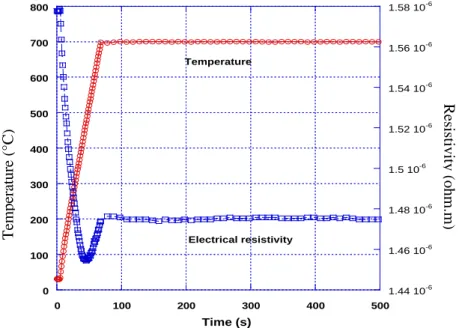
Before analyzing the transformation kinetics during isothermal treatments, we present the variations of electrical resistivity measured on heating and further holding at constant temperature. As an example, the variations obtained during

heating and the beginnings of the holding at 700oC are shown in Figure 3-1. A first

decrease in electrical resistivity is observed during heating from room temperature to 400-450oC, followed by an increase in resistivity. During the holding at 700oC, the electrical resistivity is nearly constant for the time considered in Figure 3-1.

Figure 3-1 Variations of electrical resistivity and temperature versus time during heating

to and holding at 700oC with 10oC/S heating rate

The electrical resistivity variations with time during heating is quite complex. From room temperature to nearly 400oC, a negative dependence of electrical resistivity with temperature is measured, commonly observed for different beta-metastable alloys[80,82,95,99]. At higher temperature the electrical resistivity raises with the

0 100 200 300 400 500 600 700 800 1.44 10-6 1.46 10-6 1.48 10-6 1.5 10-6 1.52 10-6 1.54 10-6 1.56 10-6 1.58 10-6 0 100 200 300 400 500 Temperature( o C) Resisitivity(oh m .m) Time (s) Temperature Electrical resistivity Resistivity (ohm.m) Temperature (°C)

(43)

increase of temperature.

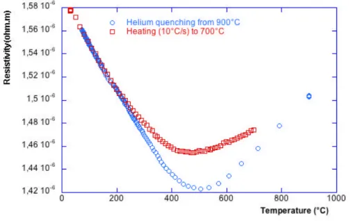
In Figure 3-2 we compare the variations in electrical resistivity measured during rapid cooling from beta temperature range to the variations in electrical resistivity

measured during heating up to 700oC. The variations on cooling present a first

decrease as temperature decreases from 900oC to 500oC. At lower temperature the

electrical resistivity increases. During cooling, no major transformation happens. Formation of an-isothermal ? phase cannot be excluded. Thus these variations are considered as a base line for the resistivity behavior on cooling without transformation. The comparison of the variations on cooling and heating leads to

similar evolution between 20oC and 200oC. At higher temperature, we do not have a

clear superposition for the two evolutions, but the global evolutions are similar. It is difficult to establish a clear correspondence of the observed variations with structural changes in the alloy. Changes in the vacancies density can for example lead to differences in the resistivity variations. In the present case, as the resistivity on heating behaves nearly similarly to the previous one on cooling we consider that the precipitation is negligible for the considered heating rate of 10oC/s. The occurrence of precipitation during heating is further discussed in Chapter 4

Figure 3-2 Variations in electrical resistivity measured on cooling from beta temperature

(44)

III.1.2. Variations of electrical resistivity with time during isothermal treatment

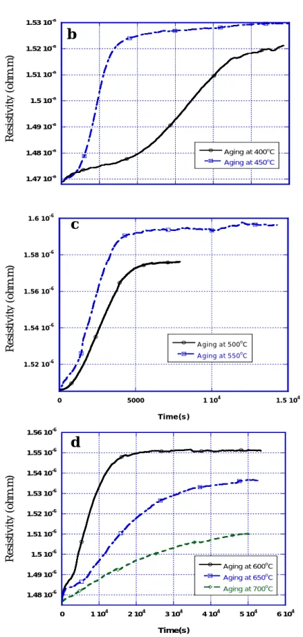
Figure 3-3 shows the variations of electrical resistivity versus time during aging

treatment for different temperatures ranging from 300oC to 700oC. It can be found

from the figure that:

(1) For each temperature, the resistivity increases with the duration of the aging time

until it reaches the maximum value and maintains constant (excepting 300oC and

350oC), which means that the phase transformation process is completed for the

corresponding isothermal aging treatment condition.

(2) For temperature varying from 650oC to 400oC, the curve has a nearly sigmoid

shape. It can be divided into different stages. The first stage is the beginning of the phase transformation. When the isothermal treatment temperature is below

550oC, the resistivity increases lowly with time while above 550oC (including

550oC) the resistivity increases at a higher rate. The required time for finishing the beginning stage of phase transformation varies with the isothermal

temperature, with a minimum of about 500s (500~550oC) and a maximum about

15000s (400oC).

a

1.42 10-6 1.43 10-6 1.44 10-6 1.45 10-6 1.46 10-6 1.47 10-6 1.48 10-6 0 1 104 2 104 3 104 4 104 5 104 6 104 7 104 8 104 Aging at 300oC Aging at 350oC Res istivity (oh m .m) Time (s) Resistivity (ohm.m)

(45)

Figure 3-3 Variations of resistivity with time during aging at different temperatures:

300~ 350°C(a), 400~ 450°C(b), 500~ 550°C(c), 600~ 700°C(d), respectively. 1.48 10-6 1.49 10-6 1.5 10-6 1.51 10-6 1.52 10-6 1.53 10-6 1.54 10-6 1.55 10-6 1.56 10-6 0 1 104 2 104 3 104 4 104 5 104 6 104 Aging at 600oC Aging at 650oC Aging at 700o_C Resistivity(ohm. m) Time(s)

d

c

b

1 . 5 2 1 0-6 1 . 5 4 1 0-6 1 . 5 6 1 0-6 1 . 5 8 1 0-6 1 . 6 1 0-6 0 5 0 0 0 1 1 04 1.5 104 A g ing at 500oC A g ing at 550o_C Resistivity(ohm.m) Tim e ( s ) Resistivity (ohm.m) Resistivity (ohm.m) 1.47 10-6 1.48 10-6 1.49 10-6 1.5 10-6 1.51 10-6 1.52 10-6 1.53 10-6 Aging at 400oC Aging at 450o C Res istivity(oh m .m) Resistivity (ohm.m)

(46)

In the second stage the electrical resistivity increases rapidly with time. The third stage is the ending stage of phase transformation during which the phase transformation is nearly finished and the trend that resistivity increases with time slows down and holds after reaching a maximum value. For the lower

(300~350oC) and higher (650oC~700oC) temperatures, the variations of

resistivity with time have more a parabolic shape.

(3) The time required to reach the maximum value for the resistivity change is dependant on the temperature: the shortest time to reach the maximum is for

550oC; the duration of the transformation increases for transformation

temperatures above 550oC as well as below 550oC.

III.1.3. Method to obtained phase transformation kinetics from in-situ resistivity variations

Resistance is a physical property of materials, which has close relation with the chemical elements and microstructure, etc. The variation trend of resistivity evolution with time corresponds to the phase transformation kinetics of the alloy during isothermal process. Previous results obtained for several titanium alloys by

Laude, Bein, Malinov, Gautier and Bruneseaux[83,100~102] for isothermal

transformation on cooling from beta range indicated a linear relationship between the variation of resistivity (relative change of resistivity) and the relative amount of α phase. This was clearly established by Bruneseaux et al comparing in-situ electrical resistivity variations with amount of alpha phase obtained by in-situ high energy X-ray diffraction[103]. A link can thus be established between the relative changes in electrical resistivity and the transformation kinetics. It is thus considered that the progress of the transformation during the isothermal process is proportional to the measured relative resistivity, and a higher increase of electrical resistivity corresponds to a higher amount of alpha phase.

Phase transformations and microstructure evolutions in metastable beta titanium alloy Ti-B19

HAL Id: tel-01749447

https://hal.univ-lorraine.fr/tel-01749447

metastable beta titanium alloy Ti-B19

Hui Chang

To cite this version:

AVERTISSEMENT

Ce document est le fruit d'un long travail approuvé par le jury de

soutenance et mis à disposition de l'ensemble de la

communauté universitaire élargie.

Il est soumis à la propriété intellectuelle de l'auteur. Ceci

implique une obligation de citation et de référencement lors de

l’utilisation de ce document.

D'autre part, toute contrefaçon, plagiat, reproduction illicite

encourt une poursuite pénale.

Contact : ddoc-theses-contact@univ-lorraine.fr

LIENS

Code de la Propriété Intellectuelle. articles L 122. 4

Code de la Propriété Intellectuelle. articles L 335.2- L 335.10

http://www.cfcopies.com/V2/leg/leg_droi.php

ACKNOWLEDGEMENTS

CONTENTS

I. INTRODUCTION

I.1.

Brief introduction of titanium alloys

[ ]

I.2.

Phase transformation in titanium alloys

(

)

{ }

( ) ( )

[ ]

( ) ( )

[ ] [ ]

{ }

{ }

[ ]

{ }

I.3.

The phase transformation kinetics of titanium alloys

(

)

( )

∫

I.4.

The aim of the present research work

II. RESEARCH SCHEME AND

EXPERIMENTAL PROCEDURE

II.1.

Research contents

II.2.

Researching routes

II.3.

Experimental materials

II.4.

Experiment methods and devices

I

U

T. Measure

(

)

? ? ? ? X? ? ? ? ? ? ?

III. ISOTHERMAL PHASE TRANSFORMATION

KINETICS AND MICROSTRUCTURE

EVOLUTIONS OF TI-B19 ALLOY

III.1.

Variations of electrical resistivity with time and further

analysis method

a

d

c

b