HAL Id: tel-02340994
https://tel.archives-ouvertes.fr/tel-02340994
Submitted on 31 Oct 2019HAL is a multi-disciplinary open access
archive for the deposit and dissemination of sci-entific research documents, whether they are pub-lished or not. The documents may come from teaching and research institutions in France or abroad, or from public or private research centers.
L’archive ouverte pluridisciplinaire HAL, est destinée au dépôt et à la diffusion de documents scientifiques de niveau recherche, publiés ou non, émanant des établissements d’enseignement et de recherche français ou étrangers, des laboratoires publics ou privés.
structures
Marco Rosatello
To cite this version:
Marco Rosatello. Contribution to the study of damping in bolted structures. Solid mechanics [physics.class-ph]. Université Paris-Saclay, 2019. English. �NNT : 2019SACLC049�. �tel-02340994�
NN
T
:20
19S
A
C
LC04
in bolted structures
Thèse de doctorat de l’Université Paris-Saclay préparée à Centrale Supélec
Ecole doctorale n◦579 Sciences Mécaniques et Energétiques, Materiaux et Géosciences (SMEMAG)
Spécialité de doctorat : Mécanique de solides Thèse présentée et soutenue à Saint-Ouen, le 5 Juin 2019, par
M
ARCOROSATELLO
Composition du Jury :
David NERON
Professeur, ENS Cachan, LMT Président
Emmanuel RIGAUD
Maître de Conférences, École Centrale de Lyon, LTDS Rapporteur
Olivier THOMAS
Professeur, ENSAM Lille, LSIS Rapporteur
Gaël CHEVALLIER
Professeur, FEMTO-ST Examinateur
Cyril TOUZÈ
Professeur, ENSTA Paris Tech, IMSIA Examinateur
Jean-Luc DION
Professeur, Supméca, Laboratoire QUARTZ Directeur de thèse
Nicolas PEYRET
Maitre de Conférences - Supméca, Laboratoire QUARTZ Co-directeur de thèse
Benoît PETITJEAN
Ingénieur Expert, Ariane Group Invité
Lionel ZOGHAIB
List of Figures vii
List of Tables ix
Acknowledgements 1
Resumé 3
Introduction 7
1 The CLIMA Project 9
1.1 Context . . . 10 1.2 Partners . . . 10 1.3 Project Goals . . . 11 1.4 Thesis Goals . . . 12 1.5 Project Mock-ups . . . 12 1.5.1 ORION Mock-up . . . 12 1.5.2 AERO Mock-up . . . 12 1.5.3 Mock-up ADR . . . 14 1.6 Conclusion . . . 15
2 Bolted structures dynamics 17 2.1 General behavior of bolted joints . . . 18
2.1.1 The monolithic-assembly comparison . . . 18
2.1.2 Bolt preload . . . 19
2.1.3 It’s all about friction . . . 22
2.1.4 Dynamic properties of bolted joints . . . 23
2.2 Friction Models for bolted structures . . . 25
2.2.1 Static friction models . . . 25
2.2.2 Dynamic friction models . . . 27
2.2.3 Hysteretic friction models . . . 29
2.2.4 Constitutive friction models . . . 34
2.2.5 A relation between Dahl and Mindlin . . . 36
2.3 A benchmark test case . . . 38
2.3.1 Nonlinear Modal Analysis of the Brake-Reuss beam . . . 38
2.3.2 The repeatability challenge . . . 40
2.3.3 The importance of exciting the nonlinearity . . . 41
2.3.4 High-detail numerical modeling . . . 42
3 A finite element connector system for bolted joints dynamics 49
3.1 FEM modeling of bolted joints . . . 50
3.1.1 Quasi-Static modeling . . . 50
3.1.2 Dynamic modeling . . . 51
3.1.3 Placing of the new connector system . . . 55
3.2 Normal contact of rough surfaces . . . 55
3.2.1 Assumptions . . . 56
3.2.2 Equations . . . 56
3.2.3 Dimensionless Equations . . . 57
3.2.4 Surface statistical properties determination . . . 58
3.2.5 Extensions and Alternatives . . . 59
3.3 Tangential Stiffness Calculation . . . 60
3.4 The Connector System . . . 62
3.4.1 Overview . . . 62
3.4.2 Connector C1 . . . 64
3.4.3 Connector C2 . . . 66
3.4.4 Preload Application . . . 68
3.5 Implementation of the connector system . . . 69
3.5.1 Objective . . . 69
3.5.2 Implementation . . . 70
3.5.3 Results . . . 71
3.6 Conclusion and Perspectives . . . 73
4 A post-processing toolbox based on Kalman Filter 81 4.1 Kalman Filter . . . 82
4.1.1 Linear Kalman Filter . . . 82
4.1.2 Nonlinear Kalman Filters . . . 83
4.1.3 Initialization of the Kalman Filter . . . 89
4.1.4 Tracking of a generic sine signal with a Kalman filter . . . 91
4.2 Kalman Filter for impact tests . . . 93
4.2.1 Model Formulation . . . 94
4.2.2 Test Case . . . 96
4.3 Kalman Filter for sweep sine tests with harmonics tracking . . . 99
4.3.1 Sweep sine testing . . . 99
4.3.2 Model Formulation . . . 102
4.3.3 Modal Identification with the FORCEVIB method . . . 105
4.3.4 Test Case . . . 106
4.4 Kalman Filter for random vibration testing . . . 109
4.4.1 Differential equations inside Kalman . . . 109
4.4.2 Linear Modal Formulation . . . 111
4.4.3 Nonlinear Modal Formulation . . . 112
4.5 Conclusion . . . 114
5 Experimental study on a complex bolted structure 117 5.1 Experimental Setup . . . 118
5.1.1 Pre-Testing . . . 118
5.1.2 Configurations and Objectives . . . 121
5.2 Experimental Results . . . 123
5.2.1 Impact Testing . . . 123
5.3 Conclusion . . . 132
Conclusion 137
A Line-Fit Method I
A.1 Method Description . . . I
A.2 Nonlinear extension . . . III
1.1 Mock-up ORION (dimensions in millimeters) . . . 13
1.2 Mock-up AERO . . . 13
1.3 Joint system between center caisson and wing . . . 14
1.4 Mock-up ADR . . . 14
2.1 Lap-joint and its corresponding monolithic . . . 18
2.2 Example of impact response difference between a bolted structure and a mono-lithic one . . . 19
2.3 Difference of dissipated energy between a bolted structure and a monolithic one 20 2.4 FEM application of preload on a lap joint . . . 21
2.5 Example of contact pressure measurement with pressure film. Stronger the color, higher the pressure. . . 22
2.6 Quasi-static traction loading of a lap-joint . . . 23
2.7 Modal behavior comparison between monolithic and assembled structures . . . 24
2.8 Static friction models . . . 26
2.9 Example of Dahl cycles for different values of the parameterα . . . 27
2.10 Example of Valanis cycle with its parameters . . . 28
2.11 General hysteresis cycle and its phases . . . 29
2.12 Jenkins element and its steady state hysteresis cycle . . . 30
2.13 Iwan Element . . . 32
2.14 Jenkins elements friction limit distribution according to Iwan and Segalman . . . 32
2.15 Contact between a plane and a sphere pressed on each other with a normal force N and with sphere subjected to tangential force T . . . 34
2.16 Mindlin and its correlated Dahl models compared for a series of micro-slip cycles 37 2.17 Brake-Reuss Beam (BRB) . . . 38
2.18 Example of frequency response function for the Brake-Reuss beam and modal parameters for the first three flexion modes . . . 39
2.19 Nonlinear behavior of the Brake Reuss Beam . . . 40
2.20 Influence of the clearance value on the BRB frequency response (zoom on the first flexion mode) . . . 41
2.21 Tested versions of the Brake-Reuss Beam . . . 41
2.22 Mode shapes of the three beams for the first three flexion modes . . . 42
2.23 Nonlinear damping ratio of the three beams for the first three flexion modes . . . 43
2.24 Comparison of friction loss factorη between BRB and SBRB . . . 44
2.25 The multi-scale properties of assemblies . . . 45
3.1 FE models for bolted joints - Source: [25]. . . 50
3.3 Multi-Connected Rigid Surfaces (MCRS) - Source: [19]. . . 52
3.4 3D contact element (left) and different distributions at the joint interface (right). Source [49]. . . 53
3.5 Whole joint approach. Source: [27]. . . 54
3.6 Example of rough profile and its asperity peak-height distribution . . . 56
3.7 Flat surface in contact with the rough one . . . 57
3.8 Evolution of dimensionless number of asperities in contact (left), true contact area (center), and normal force (right) . . . 58
3.9 Comparison of Greenwood-Williamson model with Polycarpou approximation for different values of c andλ parameters . . . 60
3.10 Comparison of different approximation of tangential stiffness with experimental benchmark data . . . 61
3.11 General bolted joint dimensions . . . 62
3.12 Connector system diagram . . . 63
3.13 Axial nonlinear stiffness of the connector C1 . . . 64
3.14 General bolt dimensions . . . 65
3.15 General washer dimensions . . . 65
3.16 C2 connector axial (right) and tangential (left) diagram . . . 66
3.17 Comparison of dimensionless joint stiffness comparison calculated with different methods . . . 67
3.18 Example of hysteresis cycle implemented in the C2 connector.α=0.3. . . 68
3.19 Preload application to the connectors . . . 69
3.20 Experimental results on the ORION mock-up . . . 70
3.21 Implementation of the developed connector on the ORION mock-up . . . 70
3.22 Example of FRF numerically calculated through the stepped sine technique with Dahl parameters deriving from theory . . . 71
3.23 Example of FRF numerically calculated through the stepped sine technique with Dahl parameters derived from theory . . . 72
3.24 Natural frequency and stiffness ratio contour map as functions of the input force amplitude and tightening torque. . . 73
3.25 Visualization of the tangential stiffness ratio between maximum and minimum tightening torque . . . 74
3.26 Numerical high-fidelity simulations on the Brake-Reuss Beam imposing modal deformations. Slip at contact interface is maximum in deep blue areas, which are far from the bolt-holes. . . 75
4.1 Example . . . 87
4.2 Initial state parameters initialization . . . 90
4.3 Illustration of the analytic signal (inspired by Feldman [5]). . . 92
4.4 SDOF nonlinear test case. m = 1Kg, c = 1Nms-1, k = 3947.8Nm-1. Iwan: Fs = 10N, Kt= 1500Nm-1,χ = −0.3, β = 0.5. . . 97
4.5 Example of Kalman filter application for impact tests. . . 98
4.6 Comparison between Kalman nonlinear identification and theory . . . 98
4.7 Natural frequency identification on the test case as function of Q and R covariances.100 4.8 SDOF system FRF obtained from sweep test at different sweep rate . . . 101
4.9 Signal and amplitude tracking on input and output with Kalman filter for the SDOF test case . . . 107
4.10 Harmonic components tracking on output signal for the SDOF test case . . . 107
4.12 Nonlinear frequency and damping evolution calculated with the FORCEVIB method
for the SDOF test case . . . 108
4.13 FRF of the Duffing SDOF system obtain through the Kalman filter procedure on a sweep sine test . . . 109
4.14 Three masses dynamic system used as a general example . . . 110
4.15 Results for the displacement and stiffness tracking for the three-masses system undergoing random excitation . . . 111
5.1 Average Driving DOF Displacement map for the AERO mock-up . . . 119
5.2 Optimal Driving Point map for the AERO mock-up . . . 120
5.3 Average Driving DOF Velocity map for the AERO mock-up . . . 120
5.4 Example of OMS method application on the AERO Mock-up. . . 121
5.5 AERO mock-up experimental boundary conditions . . . 122
5.6 Experimental mesh and accelerometers’ position for impact testing modal iden-tification. . . 123
5.7 Complex Mode Indicator Factor for the AERO mock-up in free-free conditions. . 124
5.8 First six mode shapes for the AERO mock-up in free-free conditions. . . 125
5.9 Linear modal analysis of the AERO mock-up mounted on the shaker. . . 126
5.10 Original FRF and the low-pass filtered one . . . 127
5.11 Total signal and modes contributions tracking for accelerometer A1 for a test at 800N impact force. . . 127
5.12 Tracking of natural frequencies and damping ratios in time for a test at 800N im-pact force. . . 128
5.13 Nonlinear natural frequencies and damping as a function of amplitude for the accelerometer A1. . . 129
5.14 FRF for a random excitation on the shaker in the frequency range 0-400Hz. . . . 130
5.15 Example of signal and instantaneous frequency tracking for an upward sweep of 0.05g excitation amplitude. . . 131
5.16 Comparison of FRFs obtained with the UKF at different forcing amplitudes, for upward and downward sweeps on the ABT configuration. . . 132
5.17 Nonlinear modal identification on the ABT configuration of the AERO mock-up, through the combination of Kalman filter and FORCEVIB method, fitted with four-parameter Iwan models. . . 133
5.18 Nonlinear behavior comparison based on configuration, tightening torque, and experimental campaign. . . 134
A.1 Example of Line-Fit method application on a linear 3-DOF system. . . III
A.2 Example of nonlinear Line-Fit method application on a three-masses system with an Iwan model. . . IV
3.1 Values of theλ parameter according to different authors . . . 61
4.1 Comparison of main Kalman filtering methods features . . . 89
5.1 Modal analysis results for the AERO mock-up in free-free conditions. . . 124
Getting a Ph.D. is not an easy task. However, with the right people around you, it can get a lot easier.
Firstly I would like to acknowledge the CLIMA project for founding this work and for creating an active research environment between companies and academic partners.
Then I would like to thank the figures who most influenced this work and that helped me to carry it out. The first one is my main supervisor Prof. Jean Luc Dion, who guided me in each phase of this work, always trying to bring out the best from me. I would like to thank my co-supervisor Prof. Nicolas Peyret who was always available for me, with his great knowledge of the contact physics. On the company side, I would like to thank Dr. Benoit Petitjean, my industrial supervisor at Airbus, that welcomed me in his office in Suresnes and helped me on many levels, from unveiling the secrets of the dynamics lab to giving me great technical advice thanks to his experience with jointed structures. Inside Airbus, I also would like to make a special thank you to Dr. Lionel Zoghaib, with which I had great talks about the world of research and that helped me many times during these years. A special thank you goes to Prof. Etienne Balmes, which, with his infinite knowledge of structural dynamics, made possible the construction of the finite element connector in SDTools software.
I would like to acknowledge all the members of the jury and the guests for having accepted to attend the discussion and which has shown great interest in this work. In particular, I would like to thank Prof. Emmanuel Rigaud and Prof. Olivier Thomas for carefully reviewing this the-sis and for their great insights, Prof. David Neron for having accepted to be the president of the jury, and Prof. Cyril Touzè and Gaël Chevallier for their role of examinator.
I would like to acknowledge the SANDIA Laboratory of Albuquerque New Mexico, in partic-ular, Prof. Matthew Brake, for financing and accepting my application to participate in the NOMAD Research Institute in 2016. It was a unique and essential experience for my thesis. I would also like to thank my project team members, Allen, Kelsey, and Samson, for the great moments spent in the lab.
A Ph.D. is also made of places: during these three years Supmeca, a small university with great potential and great people, has been my second family (the first one being in Italy). It’s im-portant to have nice colleagues around you during a doctorate: a very special thank you goes to Adrien C., who worked too on the CLIMA project and with whom something much deeper than a simple work relationship was developed. Mutual support in difficult moments has been crucial. Speaking of mutual support it’s impossible not to mention Emna and Reza: our cof-fee break talks really made my day on countless occasions. A huge acknowledgement goes to
Adrien G., who introduced me to the Kalman Filter and helped me to understand when it didn’t want to work. Getting out of the office, the next acknowledgment goes the team VAST, a group of dynamic people from which I’ve learned a lot. I would like to thank all the staff of Supmeca, always available and reactive to help me solve my problems, especially when I was new to the school and my French was not that good.
A particular thank you goes to a special group of friends that created in Supmeca and with which I’ve shared wonderful moments. Therefore thank you, Adrien, Alain, Alexandre, Jpal, Paul, Sophie, and Stefania.
During the period of my thesis, I had the chance of organizing the JJCAB 2017, between Sup-mèca and the CNAM. Therefore, I would like to thank the organization group Aro, Arthur, Christophe, Martin et Sylvain.
I would like to thank my family, that made the graduation day a very special one and that al-ways supported me even if I was far from them during all these years.
Finally, I would like to thank Pauline, without whom anything of this would have happened. Thank you for sharing every single moment of this adventure with me.
Introduction
La dynamique des structures assemblées est un sujet de recherche d’actualité. Plus précisé-ment, une prédiction correcte de l’amortissement apporté par les liaisons boulonnées est de-venu une condition essentiel pour un certain nombre d’applications, comme par exemple les véhicules aéronautiques et spatiaux. En effet, pour ces applications,l’utilisation de matériaux avec un coefficient d’amortissement plus élevé, comme les matériaux visco élastiques, est lim-ité par les conditions de fonctionnement. Dans ces cas, les sources principales d’amortissement proviennent des liaisons vissées, essentiellement dû au frottement qui a lieu à l’interface en-tre les composants. L’évaluation de l’amortissement apporté par les liaison vissées est le sujet principal de ces travaux.
Le problème rencontré par les chercheurs sont est le fait qu’une méthode pour la prédiction de l’amortissement d’une structure assemblée n’existe pas. Donc, les liaisons boulonnées sont conçues en tenant compte des normes existantes, mais le comportement dynamique est évalué seulement une fois que la structure a été construite, ce qui peut impliquer des pertes de temps considérables. La raison principale pour laquelle l’évaluation de l’amortissement des struc-tures assemblées est compliqué, vient du fait que son comportement est de type non-linéaire. Toutefois, la nonlinearité n’est pas toujours très marqué, ce qui permet parfois l’utilisation d’outils d’identification modale linéaire, avec quelques précautions et hypothèses.
Chapitre 1
La thèse fait partie d’un projet important appelé Projet CLIMA -Conception de LIaisons Mé-caniques Amortissantes, un projet collaboratif de recherche FUI. Ce type de projet supporte la recherche appliqué de façon transversale. En fait, il permet la connexion entre grandes, moyennes et petites entreprises, ainsi que des laboratoires de recherche.
Les objectifs du projet CLIMA peuvent être divisés en quatre aspects:
1. Conception: création et prototypage de liaisons avec un haut pouvoir dissipatifs, sans influencer l’intégrité structurelle;
2. Contrôle: développement de nouveaux capteurs et actionneurs pour mesurer et modifier les propriétés des liaisons;
3. Modélisation: développer un outil numérique pour l’optimisation de l’amortissement dans la phase de conception;
4. Évaluation: développer un set d’outils de post-traitement pour la détermination de l’amortissement non-linéaire des structures assemblées.
Les travaux présentés sont focalisés sur les objectifs de modélisation et d’évaluation. En fait, le défi d’évaluer l’amortissement dû aux liaisons vissées sera approché par deux cotés. D’une part, une formulation analytique du problème de contact à l’interface de la liaison sera présen-tée et implémenprésen-tée dans les éléments finis, afin de prédire l’amortissement dans la phase de conception. D’autre part, un set d’outils adaptés aux liaisons boulonnées sera développé pour évaluer le comportement dynamique d’une structure assemblée soumise à différents types d’excitation.
Chapitre 2
Les liaisons boulonnées, entendues comme l’utilisation d’une vis et un boulon pour connecter deux pièces, font leur apparition dès le 15ème siecle. A l’époque, ils étaient faits à la main, et c’était très difficile de faire deux filets correspondants. Aujourd’hui, les dimensions des vis, des boulons et des filets sont strictement normées, comme il est également le dimension-nement des liaisons. Toutefois, le comportement de ce type de liaisons est toujours un sujet de recherche, en particulier en ce qui concerne leur comportement dynamique.
Il peut être intéressant de comparer le comportement dynamique, en particulier concernant l’amortissement,d’une structure avec une liaison boulonnée et la même structure, mais cette fois monolithique et sans liaison. La structure boulonnée aura un taux d’amortissement plus élevé que la structure monolithique. Ce comportement est dû au frottement qui survient dans l’interface de contact. En outre, le taux d’amortissement évolue de façon non-linéaire avec l’amplitude d’excitation et il dépend de plusieurs facteurs caractéristiques des liaisons, dont le niveau de pré-charge de la vis, les dimensions de la vis, la conformabilité des surfaces en con-tact, la direction de l’excitation, la forme des modes propres sollicités et autres paramètres. Vu l’importance du frottement dans la dynamique des liaisons,les modèles principaux sont décrits, en faisant la distinction entre macro-modèles et modèles constitutifs. Les macro-modèles sont basés sur des lois empiriques et/ou des observations expérimentales, lorsque les mod-èles constitutifs dérivent de la physique du contact. Les macro-modmod-èles peuvent être divisés en modèles statiques (Coulomb, Stribeck), dynamiques (Dahl, Valanis) et hystéretiques (Mas-ing,Iwan). Une fois la description des différents modèles de frottement est faite, une liaison entre le modèle constitutif de Mindlin et le modèle hystéretique de Dahl est trouvée. Ce lien sera utilisé dans la phase de modélisation du chapitre 3.
Dans la dernière partie du chapitre 2, une structure de référence, la poutre de Brake-Reuss, est étudiée expérimentalement et numériquement, et les résultats sont montrés. Enfin, une discussion sur le caractère multi-échelle des structures assemblées est amenée.
Chapitre 3
La simulation numérique des structures assemblées n’est pas une tache facile. Le problème principal vient du fait que les liaisons représentent une petite partie de la structure, ce qui génère un problème multi-échelle, très lourd à résoudre numériquement par la méthode des éléments finis. L’autre aspect à considérer est que la physique du contact des liaisons demande une modélisation détaillée, en particulier en ce qui concerne le frottement.
Le premier objectif de ces travaux est de trouver une méthode de modélisation pour la dy-namique des liaisons boulonnées. Un état de l’art est accompli sur les techniques de modélisa-tion des liaisons boulonnées couramment utilisées. Ensuite, dans le cadre des travaux de thèse, un système original de connecteurs est développé. L’idée de ce système est de réussir à mod-éliser le comportement des liaisons à partir seulement de ses paramètres physiques
(dimen-des boulons et, le cas échéant, (dimen-des rondelles. Le deuxième décrit le contact normale et tangen-tiel entre les surfaces en contact. Pour le contact normal, le modèle de Greenwood-Williamson est utilisé, pour le contact tangentiel et le frottement, le modèle de Dahl est appliqué. Tout les paramètres des modèles sont calculés à partir des données disponibles sur la définition de la liaison.
L’implémentation du connecteur a été réalisée dans le logiciel SDTools, une toolbox de dy-namique structurelle basée sur MATLAB. Le système de connecteurs a été appliqué sur une des maquettes développées pour le Projet CLIMA, pour laquelle une campagne expérimentale a été menée. Les résultats obtenus numériquement avec le nouveau système de connecteurs ont été comparés aux données expérimentales. Les résultats ont montré que le système développé est capable de modéliser le comportement non-linéaire typiques des liaisons. Par contre, les paramètres du système a dû être recalés pour avoir une correspondance précise avec les ré-sultats expérimentaux. Toutefois, la solution développée représente un bon compromis entre precision des résultats, simplicité d’usage et implémentation pour une usage de type industriel.
Chapitre 4
Après la partie de modélisation, l’autre objectif de ces travaux est d’identifier l’amortissement d’une structure boulonnée à partir des données expérimentales. En particulier, le développe-ment d’un set d’outils adaptés aux structures assemblées et à différents types d’essais a été développé.
La base commune des méthodes développées est l’utilisation du filtre de Kalman, un outil très puissant qui, dans ces travaux, a été adapté pour amener une identification modale non-linéaire de haute precision. Le filtre a été crée par Rudolph Kalman en 1960 et il a été utilisé pour une vaste gamme d’applications, par exemple dans le secteur de la navigation, contrôle, optimisation de la trajectoire, en particulier pour de véhicules aéronautiques et spatiaux. Par définition, le filtre de Kalman est un algorithme d’estimation optimale, dont l’objectif principal est de suivre l’évolution en temps d’un système dynamique. La première formulation originel du filtre de Kalman est linéaire, mais ils existent plusieurs versions non-linéaires. Une descrip-tion étendue des différents types de filtres de Kalman est fournie dans ce chapitre.
Dans ces travaux la formulation du filtre utilisée est le Unscented Kalman Filter. Trois méth-odes d’identification non-linéaires sont développées: la première pour les essais aux chocs, la deuxième pour les essais au balayage sinus et la troisième pour les essais au sinus aléatoire. La base d’identification de ces trois méthodes développées est la suivie en temps d’un signal sinusoïdal générique par le filtre de Kalman. Ce procédé de suivie utilise le concept de signal analytique pour reconstruire le signal mesuré et extrapoler les caractéristiques modales d’un système.
Les méthodes pour les essais aux chocs et aux balayages sinus sont décrites et validées avec succès sur un cas test à 1-DDL incluant un modèle d’Iwan qui simule la non-linéarité d’une li-aison. Ensuite, une description et une petite guide sur la délicate phase d’initialisation du filtre de Kalman sont fournis avec un exemple sur le cas test. L’initialisation du filtre reste la tache plus lourde dans son utilisation, surtout parce que sans une initialisation correcte, le filtre ne convergera pas ou, encore pire, convergera sur des résultats incorrectes.
En concernant la méthode pour les essais aux sinus aléatoire, elle est décrite mais elle ne sera pas implémentée.
Chapitre 5
Tout au long du projet CLIMA, plusieurs campagnes expérimentales ont été réalisées sur plusieurs maquettes. Les méthodes développées dans le chapitre 4 ont donc été testées sur la maquette principale du projet, la maquette AERO. Une procédure précise de pre-test a été effectuée pour déterminer numériquement les meilleurs points d’excitation et de support pour la structure étudiée.
Ensuite une campagne expérimentale d’essais au choc et en balayage sinus a été réalisée. Les méthodes basées sur le filtre de Kalman ont été appliquées aux données expérimentales et les résultats sont très positifs. Pour les deux méthodes, il a été possible de visualiser la non-linéarité sur les fréquences propres et l’amortissement apportées par les liaisons boulonnées, même avec des niveaux d’amortissement très faibles. Différentes configurations de la ma-quette ont été testées, en changeant le couple des serrage des vis, le nombre de vis et après désassemblage et assemblage.
Les résultats montrent que les méthodes développées peuvent être appliquées à des cas réel et qu’elles sont très résistantes au bruit et arrivent à déterminer la non-linéarité sur des amor-tissement très faibles, de l’ordre de 0.05%.
Conclusion
La contribution principale de cette thèse a été d’explorer et d’étendre la connaissance sur la dynamique des liaisons boulonnées, dans un premier temps avec la conception d’une méthode de modélisation des liaisons et, dans un deuxième temps, avec le développement d’un outils de post-traitement originale, basé sur la technique du filtre de Kalman. Les résultats obtenus sont encourageants. Par contre, les projets futures liés à ces travaux doivent passer par une meilleure description des surfaces en contact pour la partie modélisation, et par une automatisation ou simplification de l’initialisation du filtre de Kalman.
Sometimes we give for granted aspects of our engineering life that have been around and used for centuries. This thesis is about one of them: bolted joints.
Bolts and nuts can look like basic tools of which we know everything and could even be con-sidered as a boring thesis topic. However, the static dimensioning of bolted joints is still an ongoing research topic, even if a large number of norms and directives exists. Here is where we have to introduce the dynamic part of the story. In fact, when a metallic structure under-goes a dynamical excitation, it’s important that the vibrations are damped in order to reduce their amplification at the resonances. Since metals material damping is usually very low, the damping is usually provided by the deployment of visco-elastic materials. However, there are certain applications, especially in the aeronautical and aerospace fields, where, due to the par-ticular environmental conditions, visco-elastic materials are not suitable. In these cases the main sources of damping become the bolted joints, due the friction that can take place at the contact interface of the assembled parts. Therefore, the evaluation of the bolted joints’ damp-ing potential is the main topic of this thesis.
The current problem with which researchers and engineers working on assembled structures dynamics are dealing with, is that a method to predict the damping contribution of bolted joints does not exist. Therefore, bolted joints are designed according to the existing norms, and the dynamical behavior is evaluated only after the structure has been built. Useless to say, this leads to time losses and to an iterative validation process.
The challenge of evaluating the damping due to bolted joints will be tackled from two direc-tions. On one hand, an analytic formulation of the contact problem at the bolted joint interface will be designed and implemented into finite elements, in order to predict the damping in the design phase. On the other hand, a set of tools, particularly adapted to bolted structures, will be developed in order to carefully evaluate the dynamic behavior of bolted structures undergoing different types of tests.
The main reason why the damping evaluation of assemblies is complicated, is that their behav-ior is nonlinear, ie the natural frequencies and damping coefficients are nonlinear functions of the displacement amplitude. However, we are still lucky because bolted structures are only slightly nonlinear, which means that sometimes linear identification tools can still be used, with the necessary precautions and assumptions.
In Chapter 1 the context of this work will be described, with a particular attention to the project of which this thesis is part and to the players involved.
In Chapter 2 an extensive state of the art will be provided, describing the typical nonlinear be-havior of bolted structures and how they are studied in the community orbiting around this topic. Furthermore, real examples and numerical investigations performed by the author will be supplied to give a complete and exhaustive overview of the problematic under study. Next, Chapter 3 will talk about the design of a finite element connector system to numerically model the full behavior of bolted joints. The several laws implemented in the system will be thoroughly described. Finally the numerical model will be tested and evaluated for an applica-tion on a real structure.
In Chapter 4 a nonlinear post-processing set of tools based on the Kalman filter method will be outlined and applied on simple nonlinear test cases.
Finally, in Chapter 5 the same post-processing tools will be applied on real experimental data from a test campaign on a mock-up structure developed by the project in which the thesis is inserted.
All illustrations and graphs that the reader will find throughout this thesis, except where differ-ently specified, are entirely created by the author.
The CLIMA Project
1
Contents 1.1 Context . . . 10 1.2 Partners . . . 10 1.3 Project Goals . . . 11 1.4 Thesis Goals . . . 12 1.5 Project Mock-ups . . . 12 1.6 Conclusion . . . 15Summary This thesis is part of a large project called Projet
CLIMA - Conception de LIaisons Mécaniques Amortissantes — Design of Dampening Mechanical Joints, an R&D collabora-tive FUI project. The FUI (Fonds Unique Interministeriel is a program that supports the applied research, in order to de-velop new products and services to be put on the market in the short or medium term. The interesting aspect of an FUI project is its collaborative nature: in fact, it allows connec-tions between larger established companies, smaller emerg-ing ones, universities and laboratories. In this first chapter the CLIMA project, its context, its partners and its goals are briefly described.
1.1 Context
The prediction of a structure dynamic response is a crucial task in the design process. In par-ticular, a good prediction of the structure damping is critical in order to be able to design a structure that meets specifications and, even more important, doesn’t fail under operating con-ditions. The structures interested by the project belong to the aeronautics and aerospace fields, in which the importance of accurately predicting the damping behavior is higher than in other areas of study. By being able to correctly predict the damping of an assembly it will be possible to have a better control of the vibration levels to which the structure is submitted. The latter aspect has very important industrial fall-outs. If we take for example a space launcher, it will be possible to reduce the vibrations to which its payload is submitted. In fact, the payload usu-ally consists of expensive and delicate structures such as satellites or measurement equipment that are sensitive to vibrations. Another example is a plane fuselage and the internal cockpit: if the vibrations transmitted by the joints are reduced, the comfort inside the cockpit will be improved, both mechanically and acoustically. The same is obviously valid for a car interior. The CLIMA project is not the first of its kind, but it takes place from a rich history of projects dedicated to the damping characterization of jointed structures. To give some examples:
• MAIAS: partially the precursor of CLIMA, it produced several test benches on which the first results on damping prediction have been obtained. In addition, a set of software prototypes for dynamic test post-processing have been developed and some of the tech-nologies used in the CLIMA project have been conceived during MAIAS.
• CARAB: the objective of this project was to develop and validate a set of methods and tools that can be used to optimize bolted assemblies for aerospace products. The focus of the CARAB project was mainly on the static or quasi-static behavior of bolted structures, while the CLIMA project focuses on their dynamic behavior.
• ARIAN: the project focuses on the prediction of damping in bolted interfaces between composite structures, with a particular interest on the space rocket Ariane.
• INMAT: a slightly different project, where the damping function is obtained through the development of new materials. Jointed structures are not treated.
It’s also worth noting that besides the cited French projects, there is an international commu-nity, the ASME Research Committee on the Mechanics of Jointed Structures (RCMJS), which sets the research roadmap for the community itself and regularly organizes and collaborates on a series of actions and challenges. The RCMJS is currently led by a committee consisting of David Ewins (Imperial College London), Larry Bergman (University of Illinois), Dan Segalman (Michigan State University), and Matthew Brake (Rice University). Furthermore, Supméca and FEMTO, the first being the university where this thesis was conducted and the second being a research institute partner of the CLIMA project, are active contributors of this community. The existence of many projects and of an international committee gives an idea of how im-portant is the knowledge of bolted structures dynamics and how much work is still there to be done.
1.2 Partners
A project, like any good movie, needs good actors in order to be successful. The industrial actors of the CLIMA project are:
as the EADS (Europen Aeronautic Defence and Space).
• Sopemea: a set of laboratories specialized in all range of testing services in the fields of mechanics, vibration, climate, electricity, hydraulics and electromagnetic.
• ADR-Alcen: a producer of high-precision ball bearings, special electromechanical actu-ators, and mechanism for electro-optical applications.
• Aderis: company specialized in bonding technologies through advanced polymers. • AVNIR Engineering: a mechanical engineering consultancy firm for the aerospace and
energy industry.
• CEDRAT Technologies: company specialized in smart actuators, smart sensors, mecha-tronic and detection systems.
• SDTools: a software company providing a complete structural dynamics toolbox based on MATLAB®
• Texense: a producer of high-tech embedded sensors for sports mechanics and automo-tive and aerospace industry.
Concerning the academic partners, these are:
• Supméca: an engineering school, part of the ISAE group, where this thesis was carried out.
• Femto-st: a research institute attached to the CNRS (Centre Nationale de Recherche Sci-entifique).
Each of the partners makes its expertise available to the project in order to reach the established goals.
1.3 Project Goals
The objectives of the CLIMA project can be divided into four different fields:
1. DESIGN: Create and prototype joints with a high dissipative potential by understanding the physics behind the energy dissipation. Of course, the new joints must not interfere with the integrity of the structure.
2. CONTROL: Develop new sensors and actuators for the measurement and control of the joints properties. For example, during the MAIAS project, some bolts were instrumented in order to measure the instantaneous bolt load.
3. MODELING: Develop a modeling and simulation numerical tool for the damping opti-mization of an assembly in the design phase.
4. EVALUATION: Develop a toolbox for the post-processing of different types of tests on jointed structures, capable of evaluating the nonlinear modal properties.
The array of goals fixed by the CLIMA project produces a comprehensive and exhaustive set for the analysis and design of jointed structures.
1.4 Thesis Goals
As it can be presumed, the thesis goals cannot include all of the project goals. A first selection has to be made on the type of joints that are studied. In fact, the CLIMA project involves the study of two different assembly techniques:
• Metallic joints: they put directly in contact two or more metallic interfaces.
• Viscous joints: they link metallic or composite components using glue only, or they com-bine the use of viscous materials with traditional metallic joints.
This thesis will only consider the metallic joints. Furthermore, concerning the goals set up by the project, the current work will mainly focus on the MODELING and EVALUATION fields. To accomplish the first, a FEM connector system will be developed and numerically implemented with the help of the project partner SDTools. Then, in order to accomplish the second goal, a post-processing toolbox that uses the Kalman filter theory will be developed. Both for the modeling and evaluation tasks, reference experimental data on which to validate the FEM con-nector and the post-processing toolbox will be necessary. To accomplish that, there have to be one or more reference structures on which to carry out the experimental tests. During the project, several test benches have been designed and manufactured to explore different joints technologies.
1.5 Project Mock-ups
The design of the mock-ups, directly belonging to the project, allows its members to have a set of structures around which it’s possible to create hypotheses, design specific tests, run numer-ical simulations and share their results. Four mock-ups have been developed for the CLIMA project, three of which are related to metallic joints and used in the present work. The latter will be briefly described in the next paragraphs.
1.5.1 ORION Mock-up
This structure was developed in order to have a simple configuration on which is possible to study and understand the physics behind bolted joints. The mock-up, shown in fig.1.1, con-sists of two aluminum parts linked together by three M4 bolted joints. The particularity of this mock-up is the fact that, on one of the two parts, a milling process is carried out to obtain three squared raised zones around the holes. This is done in order to let the contact take place only on the areas around the holes and avoid interactions with the rest of the surface. The mock-up it’s easy and cheap to reproduce, which makes it easier to use as a reference structure. In addi-tion, it provides a simple case to test newly developed methods and theories.
1.5.2 AERO Mock-up
The second and main mock-up of the CLIMA project is the structure shown in fig.1.2. The objective of this type of design is to reproduce the joints found in aeronautical and aerospace real applications in order to evaluate their influence on the structural dynamics behavior. The mock-up consists of a center caisson which is joined to two wings through a connecting plate and bolted joints. The chosen shape takes inspiration from the Airbus A380 wings, with the intent to make it both a satisfactory test bench and an iconic and representative object for the CLIMA project.
A ( 2 : 1 ) A 12 1 2 30 200 30 5 5 20 15 30 5 4 200 10
Figure 1.1 – Mock-up ORION (dimensions in millimeters)
the zinc as primary alloy element and it’s often used in transport applications (mainly aviation) due to its high strength-to-density ratio.
The connection between the center block and the wings is shown in fig.1.3. The upper part uses a link plate to connect the caisson to the wing. The link plate is mounted on the caisson with a row of eight M10 bolts, directly fitted in steel threaded inserts introduced in the center block. The other side of the link plate is then connected to the wing through a row of twelve titanium close tolerance bolts with a diameter of 6.35mm. The lower part directly connects the center block to the wing, again with a row of twelve titanium bolts. The nominal torque for the titanum bolts is 7Nm. In addition, the wings have been hollowed out, which was done not only to make the final structure lighter but also to be able to mount two metallic covers to test bolted joints mixed with polymers.
The wingspan of the assembly is slightly less than 2m and the total weight is close to 30kg, which makes it quite an imposing structure to test.
Figure 1.3 – Joint system between center caisson and wing
1.5.3 Mock-up ADR
The last mock-up dedicated to metallic joints is taken from the MAIAS project. The objective is to develop dissipative bolted joints for a system with high-precision ball bearings by oper-ating on the profile of the contact surfaces. The mock-up, shown in fig.1.4, is entirely made of stainless steel X105CrMo17, and it consists of a base, a mass, and a bearing ring. The latter is certainly the most interesting part of the structure because it has been designed to have the same stiffness behavior of the ball bearing present in the real system, in order to make it easier to construct a numerical model. In fact, a ball bearing would have been too difficult to correctly mesh and the related simulations too computationally expensive.
The connections studied by the project are the twelve circular bolted joints that fix the ring to the base. The idea is that, by introducing a custom designed ring between the base and the
bearingring, is possible to increase the damping of the structure.
1.6 Conclusion
The set of mock-ups described in these sections have been utilized by the project members as a reference to test different types of solutions and to advance in the knowledge of bolted structures and assemblies. After having described the nature of the project in which this thesis is placed, it’s now time to understand how bolted structures behave, what are their common features, what we know and what we don’t know yet, and how their study is approached by the international academic community interested in this subject.
Bolted structures dynamics
2
Contents
2.1 General behavior of bolted joints . . . 18 2.2 Friction Models for bolted structures . . . 25 2.3 A benchmark test case . . . 38
Summary Imagine having to build a car or a plane, or even a
simple IKEA®table without any bolts or screws: this is simply
impossible or VERY unlikely. This chapter is meant to give the reader a complete overview on the topic of bolted structures. At first, the general behavior and the properties observed till the present days will be described. Then, a review of the main methods for modeling friction in bolted joints will be carried out, since this is how the energy is dissipated and the damp-ing is provided. Finally, a simple bolted structure will be an-alyzed to consolidate the theoretical knowledge and to show the problems and the challenges in the study of bolted joints.
2.1 General behavior of bolted joints
In most of the mechanical fields and applications it’s very likely that at a certain point an engi-neer will have to decide which type of fastening method to use in order to assemble different components. The most common kinds of fasteners are nails, screws, bolts and rivets. Bolts and rivets have been used extensively in automotive and aviation applications. The difference be-tween them is that, while rivets are permanent joints, bolts and nuts provide a non-permanent way of assembling different components. The concept of using a threaded bolt and a matching nut as a fastener dates back to the 15th century [23], when they were made by hand and, be-cause of that, it was quite difficult to produce matching threaded profiles. Today there is a wide range of bolt types available for general and specific applications and, most of all, their dimen-sions are standardized. In addition, the design of bolted structures is subject to regulations and directives in order to avoid joints failure and fatal accidents.
However, even if bolted joints are commonly used in all types of engineering structures, their behavior is still a research topic, especially concerning their influence on the dynamics of the assembly.
2.1.1 The monolithic-assembly comparison
The most direct and easy way to understand the effect of bolted joints on the dynamic of a structure is to compare the behavior of a jointed structure with its corresponding monolithic one [9, 37, 47]. An illustrative example is shown in fig.2.1 where, on the left, is possible to see a lap-joint while, on the right, the corresponding monolithic version.
If we were to excite these two structures with an impact hammer, we would obtain a free vibration response like the one shown in fig. 2.2. The decay rate for the jointed model is higher than for the monolithic one, which means that the damping for the lap-joint is higher than the damping of the monolithic version. This is due to the fact that the only source of damping for the monolithic structure is the material damping, which is small for metallic materials—usually less than 0.1% ([35])—while for the jointed structure the additional damping is the result of the energy dissipated by friction at the contact interface.
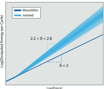
In the early 1960s Ungar [49] performed a series of tests where he used the dependence between the dissipated energy per cycle and the load amplitude to identify the source of dissipation. The dissipated energy per cycle D can be written in the following power-law form:
D ∝ Aδ (2.1)
where A is the oscillation amplitude andδ is the power-law coefficient. Ungar started to
visual-ize the results of his experiments on a log-log plot with the force or displacement amplitude on the x-axis and the dissipated energy per cycle in the y-axis. In this way, if a power-law behavior is detected, it will be looking like a straight line with a slopeδ.
(a) Jointed
(b) Monolithic
Time Displac emen t Monolithic Jointed
Figure 2.2 – Example of impact response difference between a bolted structure and a monolithic one
If we consider a linear system with viscous damping excited with an harmonic force:
m¨x + c ˙x + kx = F0sin(ωt +φ) (2.2)
the dissipated energy per cycle can be written as
D = πcΩA2 (2.3)
whereΩ is the oscillation frequency. Therefore the dissipated energy per cycle is proportional
to the oscillation frequency and to the square of the displacement amplitude. In the case of a
constant frequency, the power-law coefficient can determined asδ = 2.
If we now consider jointed structures, experiments have found a slopeδ between 2.2 and 2.8
[44, 9]. An illustrative example is provided in fig. 2.3, where it can also be observed that in the-ory, for low force amplitudes, the behavior of the bolted structure is the same as the monolith. The reason for this is that, for very low amplitudes, the contact interface is not excited enough to provide a friction damping. An important aspect to take into account is that the power-law behavior is valid only for a force amplitude lower than the maximum friction force for which the contacting surfaces of the bolted joints would totally slip — more details on that later. The difference in dissipated energy observed between the linear system and the bolted structures indicates that the latter are characterized by a nonlinear behavior. This requires us to under-stand the physical reasons behind it, in order to proceed in its analysis.
In the next sections, the important concept of bolt preload will be introduced and the role of friction in bolted joints will be discussed.
2.1.2 Bolt preload
The tricky part of having to deal with bolted joints is that even the most trivial operation can hide great uncertainty. This is the case for the bolt preload. Let’s consider a typical lap-joint, composed of two plates linked together by a bolt and a nut (see fig. 2.1a). A tightening torque T is applied to the nut while the bolt is kept still, which generates a certain traction force P in the bolt, called preload. In this way, the plates are pressed together and the integrity of the joint is
Log(Force) Log(Dissipa ted Ener gy per C ycle) Monolithic Jointed δ = 2 2.2 < δ < 2.8
Figure 2.3 – Difference of dissipated energy between a bolted structure and a monolithic one
guaranteed. The desired preload force P is determined from the proof load Fpdefined as:
Fp= AtSp (2.4)
where At is the bolt tensile-stress area and Sp is the proof strength of the bolt material. The
preload P is usually calculated as the 75% of the proof load Fpfor non-permanent connections
and 90% for permanent fasteners [10]. Once determined the preload value, the challenge is to relate it to the tightening torque to apply. The fundamental difficulty encountered in this task is to evaluate the friction forces exerted between nut and bolt threads, and between the nut and the plate surface. There are two ways of calculating the relationship between the tightening torque and the preload. On the one hand, the relationship can be calculated analytically using the physical properties of the joint, according to Motosh [33] expression:
T = P µp 2π+ µtrt cosβ+ µnrn ¶ (2.5) where:
• p is the thread pitch;
• µtis the friction coefficient between nut and bolt threads;
• µnis the friction coefficient between the face of the nut and the upper surface of the joint
plate;
• rtis the effective contact radius of the threads;
• rnis the effective contact radius between nut and joint surface;
• β is the threads half-angle.
On the other hand, the relationship can be calculated empirically using the following short-form equation:
where D is the nominal diameter and K is a dimensionless constant called nut factor. The latter is experimentally determined and can be found in tables, according to the type of joint, mate-rials and lubrication conditions [5].
It’s easy to see from eqs. 2.5-2.6 that a slight error in the choice of parameters can lead to sub-stantial errors in the determination of the tightening torque. Furthermore, there is a set of other aspects to take into account to choose the correct tightening torque, and each one of them adds uncertainty to the final real preload value:
• Tools for torque control: depending on the type of wrench chosen for the job, the accu-racy on the measured torque can vary between ±2% and ±20%
• Short-term or embedment relaxation: in the minutes following the bolt tightening, preload decreases as much as 10% or 20%
• Long-term relaxation: in the days following the bolt tightening, preload can still decrease up to 10%
• Dynamic phase relaxation: under dynamic excitation, preload can decrease up to 10%. If the necessary measures are not taken against untightening, vibrations can lead to the full loss of tightening torque.
• Multiple bolts tightening: the interactions between different bolts tightened at different times can modify their initial preload. It’s extremely important to define a correct tight-ening routine when dealing with multiple joints.
• Lubricants: their use normally increases preload accuracy, but the dynamic behavior will be affected.
• Operator: where there is human interaction there is error.
Let’s notice that from the factors listed above have been removed all the ones related to bad design and faulty components. By considering all the factors, it’s easy to understand how com-plicated is it to accurately determine and apply the preload.
“If certainty you need in clamp, just make sure those bolts are damp.” J. H. Bickford
This is also a crucial aspect for the determination of dynamic properties of bolted structures, since the real preload determines the contact properties at the joint interfaces.
Once defined the preload and relative tightening torque, it’s time to understand what happens at the joint level once the torque has been applied. This will come in handy later to understand the energy dissipation mechanism. In fig. 2.4 is shown a FEM simulation of a preload applied on a simple lap-joint. On the left the stress distribution in the bolt and plates cross-sections is visualized. A frustum shape can be recognized in the plates stress distribution: in bolted joints theory this zone is called Rotscher’s cone [42], which is a property used to analytically calculate the joint member stiffness [25, 5, 10, 51, 29].
Figure 2.5 – Example of contact pressure measurement with pressure film. Stronger the color, higher the pressure.
On the right is shown the contact pressure distribution at the plates interface: the latter is max-imum at the hole edge and it gradually decreases as the radius becomes larger. The radius for which the contact pressure tends to zero theoretically corresponds to the larger radius of the frustum. Experimentally, the contact pressure distribution can be measured thanks to pres-sure meapres-surement films [3, 36, 1] inserted between the plates before preloading the joint: an example is shown in fig. 2.5.
2.1.3 It’s all about friction
As we have seen in section 2.1.1, a jointed structure dissipates more energy than its correspond-ing monolithic version. This difference in dissipated energy is due to the friction that occurs between the surfaces in contact.
In order to understand the dissipation mechanism, the quasi-static behavior of a simple lap-joint subjected to an increasing traction force applied at the plates extremities will be con-sidered. Fig. 2.6 shows the typical nonlinear force-displacement law. The contact surface is considered as the annular surface around the plates hole. Three phases can be distinguished:
1. Micro-slip or Partial slip: in this phase the annular surface can be divided in two differ-ent regions:
• Stick zone, indicated by a dark blue dotted fill, where the contact pressure is higher enough to guarantee that there is no relative displacement between the plates. • Slip zone, indicated by a light blue dotted fill, where the tangential force locally
overcomes the friction limit and a small displacement can take place in this region. At the beginning of the force application the stick zone corresponds to the full annular contact surface. As the force becomes larger, an annular slip region grows from the ex-ternal radius of the contact surface to the inside, gradually replacing the stick region. In some of the literature ([44, 1]), the micro-slip term is reserved for the situation in which the slip region is much smaller than the total contact area, while the partial slip follows this phase. However, the boundaries between micro-slip and partial slip are not clearly defined.
2. Macro-slip: the tangential force has reached the friction force limit and the stick zone has been entirely replaced by the slip zone. At this point the force remains constant and a relative macro-displacement occurs between the plates.
3. Pinning: this last phase occurs when the displacement between the plates reaches the value of the bolt-hole clearance, which means that the bolt shank comes into contact with the hole wall. The force starts to grow again and a nonlinear bolt-hole contact stiff-ness is defined.
The evolution described here is a theoretical one. In reality, there are several practical diffi-culties that can be encountered performing these kind of tests and the curves obtained can
Tangen tial F or ce Displacement Pinning Macro-Slip Micro-Slip Stick Zone Slip Zone
Figure 2.6 – Quasi-static traction loading of a lap-joint
be quite different from the theory. However, the friction energy dissipation mechanism is the same for all types of joints configurations: where there are two surfaces in contact, there can be friction.
Quasi-static load experiments on bolted joints performed by Sandia National Laboratories [1] have observed the curve described in this section. However, since we are interested in their dynamics, in the next section we will discuss the non-linearity generated by friction on modal parameters such as natural frequency and damping.
2.1.4 Dynamic properties of bolted joints
The effect of friction on dynamic properties of built-up structures is an on-going research topic [21, 22, 52, 32]. In fact, friction generates hysteretic effects and stick-slip behaviors, which are complex to model and identify. The goal of this section is to provide the standard modal be-havior of a bolted structure, as a function of input force or displacement amplitude.
Now, bringing the comparison between a monolithic and a jointed structure to a modal level, it will be possible to understand the type of non-linearity affecting the single modes [39]. If the external input effectively excites the joints, the typical nonlinear behavior of the Frequency Response Function (FRF) will be similar to the one of fig. 2.7a. The FRF corresponding to the monolithic linear structure, indicated by the top-right arrow, doesn’t depend on the input am-plitude. Regarding the jointed structure, the FRFs obtained at increasing levels of input force generally follow the behavior that goes from the dark blue curve to the orange one.
When modal parameters are calculated, it’s possible to generate the nonlinear curves for natu-ral frequency and damping as a function of force or displacement amplitude, shown in figs. 2.7b, 2.7c — please note that the scale of their horizontal axes is logarithmic. By keeping in mind the quasi-static behavior previously described in fig. 2.6, it’s important to notice that in this case the pinning phase is not considered.
Looking at the nonlinear frequency curve of fig. 2.7b, two clear boundaries can be distinguished: • LOW amplitude: the natural frequency of the jointed structure tends to the one of the
monolithic structure — or at least to the linear one.
Frequency
FRF M
ag
nitude
Monolithic
Jointed - Micro Slip Jointed - Macro Slip
Force
(a) FRF nonlinear behavior for an SDOF system with friction
Na tur al F requenc y ωN Log(Amplitude) Monolithic Jointed Full-Slip Frequency Macro-Slip (b) Natural Frequency Log(Amplitude) Damping ζN Monolithic Jointed Macro-Slip (c) Damping Ratio
Figure 2.7 – Modal behavior comparison between monolithic and assembled structures
full-slipfrequency, which is lower than the low amplitude linear one.
Therefore, the natural frequency shows a softening behavior, which means that it decreases with the amplitude of oscillation.
Moving our attention to the nonlinear evolution of the damping ratio, the first aspect that we notice is that there is a value of the amplitude for which the damping ratio is maximum. After its maximum value, the damping ratio tends to the linear value again. This is due to the fact that, in order to keep the macro-slip regime for higher displacements, the ratio between the energy to provide to the system and the dissipated one becomes higher. The damping ratio non-linearity is used, for example, in under-platform damper for turbine blades [43, 36], in or-der to optimize the energy dissipation and reduce the vibration amplitude, which is the main cause of blade failure. However, for the application in bolted joints, there are some other as-pects to take into account. The most important one is the position of the macro-slip limit in the frequency and damping nonlinear curves. It can be observed that the macro-slip limit is placed quite before the maximum damping value. This means that, in order to maximize the damping
in bolted joints, they would have to operate in the macro-slip regime. However, a joint oper-ating in macro-slip will normally fail in its structural task. An idea could be to design a series of joints with a structural task and another series that instead have an energy dissipation task. Another factor to take into account is the pinning, which would provide an additional contact stiffness non-linearity—not shown here—in the macro-slip regime.
2.2 Friction Models for bolted structures
Friction plays a very important role in the dynamics of bolted structures. If we consider the equations of motion of a structure with friction nonlinearities we can write:
M ¨x + C ˙x + Kx + Ff(x, ˙x) = Fe (2.7)
where:
• M, C, and K are respectively the linear mass, viscous damping, and stiffness matrices; • ¨x, ˙x, and x are respectively the acceleration, velocity, and displacement vectors;
• Feis the external excitation on the system;
• Ff is the vector of internal nonlinear forces due to friction, function of x and ˙x.
Through the years, many different friction models have been developed. They can usually be divided into two main categories: macro-models and constitutive models. Macro-models are based on empirical and experimental observations, while the constitutive ones are derived from the contact theory in order to physically describe the stress-strain relationship in the con-tact region. In addition, in macro-models it’s possible to make a distinction between three categories: static, dynamic, and hysteretic [34, 22, 4]. Since the role of friction in bolted struc-tures is crucial, in the next section will be provided examples of the most used friction modeling techniques, divided by categories.
2.2.1 Static friction models
Static models are the oldest and simplest approaches to describe friction. The assumption is that the force is a static function of the difference in velocity between the two surfaces in contact.
2.2.1.1 Coulomb
The most representative and iconic friction model of this category is the one developed by
Coulomb in the 18th century. The method essentially defines the friction force Ff as a force
that opposes to the motion and that can be written as:
Ff = µN
v
|v| (2.8)
whereµ is the friction coefficient, N is the normal force pressing the body surfaces together,
and v is the relative velocity between the two surfaces. It’s also possible to define the friction
limit force Fc = µN. The curve relative to this simple law is shown in fig. 2.8a. Modifications
can be applied to this model. For example, it’s possible to consider an additional viscous force
coefficient Fv, for which the total friction force becomes:
Ff = µN
v
The name of Coulomb is one of the 72 names carved into the Eiffel tower.
This law is represented in fig. 2.8b. Experiments have shown that the normal force N and
the friction coefficientµ depend on the velocity. In particular, it is known that the friction
coefficient, when the slip velocity |v| = 0, is higher than the friction coefficient when |v| 6= 0
[40]. In the first case we refer to the static friction coefficientµs, while in the second case we
refer to the dynamic friction coefficientµd. This behavior is called stiction, which is short for
static friction, and it’s possible to define the stiction force Fs= µsN. The relative curve for the
Coulomb model with stiction can be observed in fig. 2.8c.
2.2.1.2 Stribeck
In his experiments on roller bearings, Stribeck [48] observed that, after reaching the stiction
force Fs, the friction force is not discontinuous, but it has a continuous behavior that can be
expressed by the following nonlinear law: Ff =
h
Fc+ (Fs− Fc)e−(v/vs) δsi v
|v|+ Fvv (2.10)
where vs is a parameter called Stribeck velocity that can be identified from experiments. An
example of curve described by eq. 2.10 it’s shown in fig. 2.8d. Sometimes the curve can be asymmetrical.
Other successful static friction models that have been developed can be found in the works of Karnopp [28] and Armstrong [2].
v Ff +μN -μN (a) Coulomb v Ff +μN -μN (b) Viscous Coulomb v Ff +μdN +μsN -μdN -μsN
(c) Coulomb with stiction
v Ff
(d) Stribeck
2.2.2 Dynamic friction models
Dynamic friction models are particularly used in the field of control engineering in order to compensate for the effect of friction in mechanical system, with the goal of designing high-precision servo mechanisms. These models are based on the introduction of internal state variables that can vary in time and they lead to differential equations describing the friction behavior.
2.2.2.1 Dahl
Dahl friction model [16] was introduced in 1968 to study the rolling friction in ball bearings. Dahl’s main idea was to use the materials stress-strain curve of classical solid mechanics in
order to model friction. Considering T to be the friction force and Tc = µN its critical value
according to Coulomb’s law, Dahl’s model general form can be written as: dT d x = σ · 1 −TT c ˙x | ˙x| ¸α (2.11)
whereσ is the stiffness, which represents the slope of the curve at T = 0, and α is a parameter
that determines the shape of the curve and it’s usually taken asα = 1 for simplicity.
It’s possible to see that in this model the friction force is only function of the displacement x and of the sign of the velocity ˙x. However, in the general form of eq. 2.11 the friction force T is expressed as a derivative in the displacement x. By dividing both sides of the equation by d t, is possible to obtain an expression that is more useful for time integration:
˙T = σ ˙x·1 −TT c ˙x | ˙x| ¸α (2.12) In fig. 2.9 are shown examples of Dahl hysteresis cycles obtained by imposing a cyclic
displace-ment of amplitude xmax for different values of the parameterα. For α ≥ 1, there are no
prob-lems of existence for the term between parentheses of eq. 2.12. However, for 0 < α < 1, in the event that the term inside the parentheses becomes negative throughout the cycle, the value of the force T is imposed to be the friction limit force Tc.
x T TC = 0.5 = 1 = 2 σ
2.2.2.2 Valanis
The Valanis model [50] was initially developed to deal with elasto-plastic materials under cy-cling loading. Then, more in the interest of this work, it has been successfully applied to jointed structures and contact interfaces [21, 36]. The Valanis model is described by the followin non-linear first-order equation:
˙T = E0˙x · 1 +Eλ 0 ˙x | ˙x|(Etx− T) ¸ 1 + κλ E0| ˙x|(Etx− T) (2.13) with: λ = E0 µN µ 1 − κEλ 0 ¶ (2.14)
With the help of fig. 2.10, obtained with eq. 2.13 by imposing a cyclic displacement of amplitude
xmax, it’s possible to distinguish the different parameters composing the Valanis model:
• E0: Stick stiffness. This is the initial stiffness at full stick conditions;
• Et: Slip stiffness. This is the stiffness at full slip conditions. In fact, experiments on
lap-joints observed that, during the macro-slip phase, the force is not constant and equal to the limit friction force but it’s characterized by a certain stiffness [21]. The latter can also be easily implemented for the Dahl model by considering an additional stiffness in parallel.
• κ: Micro to macro-slip transition coefficient (0 < κ < 1). For low values the transition between micro-slip and macro-slip is more gradual. A comparison between two values ofκ is shown in fig. 2.10.
With its small set of parameters and its simple implementation in dynamic systems, the Valanis model is a truly versatile tool for the modeling of friction in bolted structures.
Obviously, Dahl and Valanis are not the only dynamics models, but they are the most relevant
x T κ = 0.2 κ = 0.95 E0 Et