HAL Id: hal-01109181
https://hal.archives-ouvertes.fr/hal-01109181
Submitted on 25 Jan 2015
HAL is a multi-disciplinary open access
archive for the deposit and dissemination of
sci-entific research documents, whether they are
pub-lished or not. The documents may come from
teaching and research institutions in France or
abroad, or from public or private research centers.
L’archive ouverte pluridisciplinaire HAL, est
destinée au dépôt et à la diffusion de documents
scientifiques de niveau recherche, publiés ou non,
émanant des établissements d’enseignement et de
recherche français ou étrangers, des laboratoires
publics ou privés.
biogeochemistry: lessons for geo-engineering and natural
variability
Sébastien Dutreuil, L Bopp, A Tagliabue
To cite this version:
Sébastien Dutreuil, L Bopp, A Tagliabue. Impact of enhanced vertical mixing on marine
biogeo-chemistry: lessons for geo-engineering and natural variability. Biogeosciences, European Geosciences
Union, 2009, 6, pp.901 - 912. �10.5194/bg-6-901-2009�. �hal-01109181�
www.biogeosciences.net/6/901/2009/
© Author(s) 2009. This work is distributed under the Creative Commons Attribution 3.0 License.
Biogeosciences
Impact of enhanced vertical mixing on marine biogeochemistry:
lessons for geo-engineering and natural variability
S. Dutreuil1,2, L. Bopp1, and A. Tagliabue1
1Laboratoire des Sciences du Climat et de l’Environnement, IPSL-CEA-CNRS-UVSQ Orme des Merisiers, Bat 712,
CEA/Saclay, 91198, Gif sur Yvette, France
2Ecole Normale Sup´erieure, 45 rue d’Ulm, 75005 Paris, France
Received: 28 October 2008 – Published in Biogeosciences Discuss.: 5 January 2009 Revised: 2 April 2009 – Accepted: 24 April 2009 – Published: 25 May 2009
Abstract. Artificially enhanced vertical mixing has been
suggested as a means by which to fertilize the biological pump with subsurface nutrients and thus increase the oceanic CO2sink. We use an ocean general circulation and
biogeo-chemistry model (OGCBM) to examine the impact of arti-ficially enhanced vertical mixing on biological productivity and atmospheric CO2, as well as the climatically significant
gases nitrous oxide (N2O) and dimethyl sulphide (DMS)
dur-ing simulations between 2000 and 2020. Overall, we find a large increase in the amount of organic carbon exported from surface waters, but an overall increase in atmospheric CO2 concentrations by 2020. We quantified the individual
effect of changes in dissolved inorganic carbon (DIC), alka-linity and biological production on the change in pCO2 at
characteristic sites and found the increased vertical supply of carbon rich subsurface water to be primarily responsible for the enhanced CO2outgassing, although increased alkalinity
and, to a lesser degree, biological production can compensate in some regions. While ocean-atmosphere fluxes of DMS do increase slightly, which might reduce radiative forcing, the oceanic N2O source also expands. Our study has
impli-cations for understanding how natural variability in vertical mixing in different ocean regions (such as that observed re-cently in the Southern Ocean) can impact the ocean CO2sink
via changes in DIC, alkalinity and carbon export.
Correspondence to: L. Bopp
1 Introduction
In the context of rising anthropogenic emissions of carbon dioxide (CO2)and increasing atmospheric CO2
concentra-tions, the ocean is a significant CO2 sink (on the order of
2 Pg yr−1 over the 1990s (Denman, et al., 2008)). The so-called biological pump is one important process by which the ocean can take up atmospheric CO2 and results from
the surface water fixation of CO2into organic matter during
photosynthesis and subsequent sinking and remineralisation at depth (Volk and Hoffert, 1985). Accordingly, some geo-engineering proposals seek mitigate for rising atmospheric CO2by increasing the efficiency of the biological pump and
hence also the oceanic sink for atmospheric CO2. In the
past, such proposals tended to focus on the artificial fertil-ization of ocean productivity by the micronutrient iron (Fe) (e.g., Markels and Barber, 2000; Leinen, 2008; Lampitt et al., 2008), which limits phytoplankton productivity in certain oceanic regions (such as the Southern Ocean) (Boyd et al., 2000). Although mesoscale field experiments have shown that the addition of Fe can augment phytoplankton biomass, the increased flux of organic carbon to deep waters (termed “export”) is often very difficult to verify in situ (de Baar et al., 2005; Boyd et al., 2007). In addition, experiments with numerical models have shown that the links between Fe, phy-toplankton productivity, carbon export and atmospheric CO2
are by no means straightforward (e.g., Arrigo and Tagliabue, 2005; Aumont and Bopp, 2006), and might have unintended adverse consequences for ocean ecosystems and climate (Jin and Gruber, 2005; Cullen and Boyd, 2008).
A more recent proposal to increase the strength of the ocean’s biological pump concerns the artificial mixing of nutrient-rich deep waters with nutrient-poor surface waters
via mechanical pipes (Lovelock and Rapley, 2007). In a nut-shell, the idea seeks to mimic the natural upwelling systems that are typified by high levels of productivity. However, as seen for Fe, the practicalities are not likely to be straightfor-ward. For example, deep waters are rich in both nutrients and respired CO2, which can outgas to the atmosphere and might
offset any gains from the fertilization of productivity (Shep-herd et al., 2007). In addition, the partial pressure of CO2
(pCO2)in surface waters, which drives the rate of exchange
with the atmosphere (in addition to winds), is a positive func-tion of the concentrafunc-tion of total dissolved inorganic carbon (DIC) and sea surface temperature, and a negative function of alkalinity (Zeebe and Wolf-Gladrow, 2001). Artificial mix-ing or artificial upwellmix-ing will directly impact the profiles of temperature, DIC and alkalinity, while the secondary effects on biological productivity will also influence surface concen-trations of DIC and alkalinity. Notable associated effects in-clude potential modifications of ocean food webs resulting from the fertilization of ocean productivity, which often al-ters the dominant phytoplankton species (e.g., de Baar et al., 2005), or potential modifications of N2-fixation that has been
discussed recently and for which the net effect of an artificial upwelling remains unclear (Karl and Letelier, 2008; Fennel, 2008). Moreover, the concentrations of other climatically important gasses, such as nitrous oxide (N2O) and dimethyl
sulphide (DMS) will probably also be altered by the deliber-ate enhancement of ocean mixing. Accordingly, a complex set of interactions will ultimately resolve the impact of a suite of pipes on atmospheric CO2in a given region of the ocean.
Testing and quantifying the net effect of such a widespread deployment of ocean pipes on atmosphere-ocean fluxes of CO2, as well as the additional perturbations to ocean
ecosys-tems and other climatic gases, in the field would be a signif-icant challenge. Nevertheless, mechanistic models of ocean biogeochemistry that represent the requisite processes in a relatively detailed fashion can provide a valuable framework within which to address these questions. In doing so, we can also learn about the impact of natural variability in ocean mixing (typically driven by climate oscillations) on the ocean carbon cycle.
In this study, we mimic the effect of an array of ocean pipes in an ocean general circulation and biogeochemistry model (OGCBM) and address the regional and global im-pact on carbon export, CO2fluxes, as well as phytoplankton
species composition, N2O, and DMS. In order of importance,
we find that the overall effect of artificially mixing the ocean is a function of the mixing of 1) DIC, 2) alkalinity, and 3) nu-trients and associated biological production. Notwithstand-ing regional heterogeneity, the mixNotwithstand-ing of natural DIC is the dominant effect on atmospheric CO2increase which is then
decoupled from the elevated biological productivity. DMS fluxes to the atmosphere increase in line with changes in car-bon export, whereas the oceanic source of N2O responds to
the interactions between export and mixing in governing sub-surface oxygen (O2)concentrations.
2 Methods
2.1 Biogeochemical model description
In this study, we use the Pelagic Interaction Scheme for Car-bon and Ecosystem Studies (PISCES) ocean biogeochemi-cal model. As a detailed description of the model parame-terizations is given in Aumont and Bopp (2006), the model is only briefly presented here. The model has 24 com-partments, including four living pools: two phytoplankton size classes/groups (nanophytoplankton and diatoms) and two zooplankton size classes (microzooplankton and meso-zooplankton). Phytoplankton growth can be limited by five different nutrients: nitrate, ammonium, phosphate, silicate and iron. Diatoms differ from nanophytoplankton by their need for Si, a higher requirement for Fe and a higher half-saturation constant (because of their larger mean size). For all living compartments, the ratios between C, N and P are kept constant. On the other hand, the internal concentra-tions of Fe for both phytoplankton groups and Si for diatoms are prognostically simulated as a function of nutrients and light. There are three nonliving compartments: semilabile dissolved organic matter (with remineralisation timescales of several weeks to several years), small and large sinking par-ticles. The two particle size classes differ in their sinking speeds (3 m/d for the small size class and 50 to 200 m/d for the large size class). While constant Redfield ratios are im-posed for C/N/P, the iron, silicon and calcite pools of the particles are fully simulated. As a consequence, their ratios relative to organic carbon are allowed to vary.
In addition to the version of the model used in Aumont and Bopp (2006), we also include here a prognostic mod-ule computing DMS seawater concentrations and DMS air-sea fluxes. This module is described in detail in Bopp et al. (2008). In brief, particulate dimethylsulfonopropionate (pDMSP), the main precursor of DMS in seawater, is com-puted from the carbon biomass of the two phytoplankton groups (diatoms and nanophytoplankton) via group-specific sulphur (DMSP)-to-carbon (S/C) ratios. Then, pDMSP is released to the water column as dissolved DMSP (dDMSP) via three different processes: grazing by zooplankton, exu-dation by phytoplankton, and phytoplankton cell lysis. Once released into water, we assume that bacterial activity instan-taneously transforms dDMSP into DMS, with a dDMSP-to-DMS yield computed as a function of the bacterial nutrient stress. Simulated DMS losses are due to bacterial and pho-tochemical processes and ventilation to the atmosphere. For ventilation to the atmosphere, the gas exchange coefficient, kg, is computed using the relationship of Wanninkhof (1992) and the Schmidt number for DMS calculated following the formula given by Saltzman et al. (1993).
Finally, we also include here the module of the oceanic N2O proposed by Suntharalingham et al. (2000) to
com-pute N2O seawater concentrations and air-sea fluxes. N2O is
is as follows:
∂
∂t[N2O] = −∇ · ([N2O]v) + ∇z· (kz∇z[N2O]) +∇l· (kl∇l[N2O]) + JN2O+FN2O
The first three terms on the right-hand side represent ad-vection, vertical and lateral diffusion, JN2O represents the biological sources of N2O and FN2O is the flux of N2O across the air-sea interface. We follow Suntharalingham et al. (2000) and we assume no N2O production in the euphotic
zone (JN2O=0). In the aphotic zone, N2O is produced when ammonium is oxidized to nitrate (nitrification pathway) and when organic nitrogen is converted to N2O at low O2
concen-trations (denitrification pathway). Again, we follow Sunthar-alingham et al. (2000) and parameterize the N2O source term
to be a function of the O2concentration and O2consumption. JN2Ois given by
JN2O=α·[O2·consumption]+β·f (O2) · [O2·consumption]
where α and β are scalar multipliers and f (O2) a
func-tion of [O2] such that N2O production is maximum at
[O2]=1 µmol/L (denitrification pathway). Values for the
scalars α and β have been taken from simulation OX.5 of Suntharalingham et al. (2000). N2O is lost to the atmosphere
via gas exchange, the gas exchange coefficient, kg, being computed using the relationship from Wanninkhof (1992) and the Schmidt number for N2O.
In order to assess the impact of our mixing experiments on atmospheric concentrations, we use a well-mixed box model of the atmosphere that simulates the evolution of the atmo-spheric CO2and N2O concentrations.
2.2 Simulations
Our OGCBM couples the PISCES model to the dynami-cal ocean model ORCA2-LIM, which is based on both the ORCA2 global configuration of OPA version 8.2 (Madec et al., 1998) and the dynamic–thermodynamic sea-ice model developed at Louvain-La Neuve (Fichefet and Morales Maqueda, 1997). The ocean model has a mean horizontal resolution of 2◦by 2◦cos φ (where φ is the latitude) with a meridional resolution that is enhanced to 0.5◦at the equator. The model has 30 vertical levels (increasing from 10 m at the surface to 500 m at depth); 12 levels are located in the top 125 m.
In this study, we have used the same forcing fields as those of Aumont and Bopp (2006) and run an “offline” version of the PISCES following a very similar experimental design to that described in Aumont and Bopp (2006) and Bopp et al. (2008). We performed a climatological simulation run to quasi-equilibrium (for 3000 years), and then patchy mixing experiments and regional mixing experiments for the sub-Arctic Pacific, the Southern Ocean and the Equatorial Pacific. For all the mixing experiments and in an attempt to mimic the impact of ocean pipes on biogeochemistry, we have increased
the vertical diffusivity coefficient Kzfor all biogeochemical
tracers, down to 200 m (which is in line with the proposed di-mensions of mechanical pipes (Lovelock and Rapley, 2000)). Accordingly, all passive tracers are mixed permanently from the surface to at least 200 m, which would be broadly simi-lar in terms of net transport to adding both an artificial up-welling and downup-welling velocities of 0.1 m/s. All the other physical/dynamic forcing variables are unchanged (in par-ticular, we do not simulate any change in the mixed layer depth). For the patchy mixing experiments, the mixing sites are worldwide and represent one grid cell every 20◦in lon-gitude and every ∼10◦in latitude. In order to examine the impact of restricting mixing to a larger, but geographically constrained, region we performed “regional mixing experi-ments” in idealized locations (sub-Arctic Pacific, Southern Ocean, and equatorial Pacific). As such enhanced mixing is enforced for the entire region in question, 30◦N to 44◦N
and 124◦W to 154◦W, 40◦S to 60◦S , and 15◦S to 1◦N
and 74◦W to 124◦W, for the sub-Arctic Pacific, the South-ern Ocean and the Equatorial Pacific respectively. In addi-tion, we also performed a global mixing experiment, where the entire global ocean is mixed to at least 200 m. All ex-periments are carried out for 20 yrs, starting in 2000. Atmo-spheric CO2 and N2O are updated at the end of each year
using fossil-fuel emissions (SRES98-A2, Nakisenovic et al., 2000), biospheric carbon fluxes (Dufresne et al., 2002) and the air-sea fluxes from our ocean model for CO2, and N2O.
3 Results and discussion 3.1 Model mean state
The objective here is not to present an exhaustive validation of the model results. A detailed description of the model mean state can be found in Aumont and Bopp (2006) for car-bon, nutrients and biota and in Bopp et al. (2008) for the DMS cycle. We illustrate here some aspects of the model that are relevant to the present study.
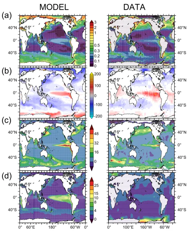
The modeled annual-mean chlorophyll distribution is compared to SeaWiFS satellite observations (Fig. 1a) and the observed patterns are qualitatively reproduced. Chlorophyll concentrations are too low in the subtropical oligotrophic gyres. In the equatorial Pacific and the Southern Ocean, the model reproduces the moderate chlorophyll levels associated with elevated macronutrients (typical of High Nutrient Low Chlorophyll regions). In the Southern Ocean however, the simulated chlorophyll concentrations appear to be too high. In the sub-Arctic Pacific Ocean, chlorophyll concentrations are generally underestimated, mainly because of deficiencies in the modeled ocean dynamics. Global annual-mean pri-mary and export productions amount to 41 and 8 Pg C y−1, respectively, which is in the range of estimations based on observations (Carr et al., 2006; Schlitzer et al., 2000).
MODEL
DATA
3 2 1 0.5 0.3 0.2 0.1 0 200 -200 48 32 16 0 15 10 25 8 4 0 0 100 -100 0° 60°E 180° 60°W 0° 0° 100°E 160°W 60°W 40°N 0° 40°S 40°N 0° 40°S 40°N 0° 40°S 40°N 0° 40°S 40°N 0° 40°S 40°N 0° 40°S 40°N 0° 40°S 40°N 0° 40°S(a)
(b)
(c)
(d)
FIGURE 1
Fig. 1. Spatial maps of modeled (left hand panels) and observed (right hand panels) (a) surface chlorophyll a (µg l−1), (b)surface 1pCO2 (ppm), (c) the ocean to atmosphere N2O flux (g N m−2yr−1), and (d) surface DMS (nM).
The modeled annual-mean air-to-sea gradient in pCO2
(1pCO2)is compared to the recently published climatology of Takahashi et al. (2008) (Fig. 1b). Again, the observed pat-terns are well reproduced by the model. Regions with posi-tive 1pCO2(oceanic sources of CO2to the atmosphere) are
in the Equatorial Pacific, the tropical Atlantic, the Arabian sea and along the Antarctic shelves. Regions with negative
1pCO2(oceanic sinks for atmospheric CO2)are simulated
in the mid-latitudes of all oceanic basins and in the high
lat-itudes of the Northern Hemisphere. The annual-mean atmo-spheric CO2sink is 2.3 Pg C y−1for 1990–1999, which is in
line with the recent IPCC estimates of 2.2±0.4 Pg C y−1for
the same period (Denman et al., 2008).
The modeled annual-mean N2O fluxes from the ocean to
the atmosphere are compared to the climatology of Nevi-son et al. (1995, Fig. 1c). The observed patterns are well reproduced by the model. High emissions of N2O are
400 300 200 100 0 -100 -200 -300 -400 0.2 0.1 0 -0.2 -0.1 0.1 0.2 0 -0.2 -0.1 100 200 0 -200 -100
60°E 120°E 180° 120°W 60°W 0° 60°E 60°E 60°S 0° 60°N 60°S 0° 60°N 120°E 180° 120°W 60°W 0° 60°E
(a)
(c)
(b)
(d)
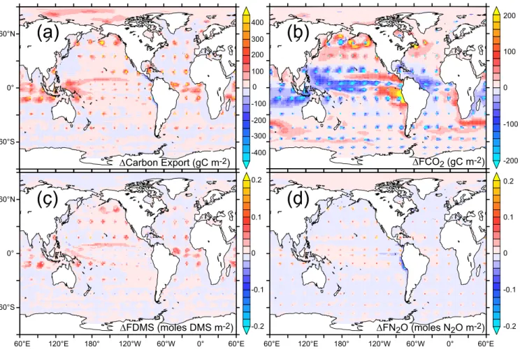
DCarbon Export (gC m-2) DFN2O (moles N2O m-2) DFCO2 (gC m-2) DFDMS (moles DMS m-2)FIGURE 2
Fig. 2. Spatial maps of the cumulative anomaly (over 20 years) in (a) carbon export (g C m−2), (b) ocean CO2uptake (FCO2, g C m−2),
(c) ocean to atmosphere DMS flux (FDMS, moles DMS m−2), and (d) ocean to atmosphere N2O flux (FN2O, moles N2O m−2).
in the North Pacific and Atlantic, and in coastal upwelling zones (e.g., Arabian Sea, Chile-Peru upwelling). Deficien-cies already identified in the comparison with SeaWiFS sur-face chlorophyll also translate into deficiencies in terms of N2O fluxes. This is the case in particular for the eastern
Sub-arctic Pacific where simulated N2O fluxes are clearly
under-estimated. Overall, the modeled N2O annual mean flux is
3.1 Tg N y−1, which is in good agreement with the recent IPCC estimate of 3.8±2.0 Tg N y−1(Denman et al., 2008).
Modeled annual-mean DMS sea-surface concentrations are compared to the climatology of Kettle and Andreae (2000) (Fig. 1d). A variety of different approaches have been use to produce sea surface DMS climatologies (see Belviso et al., 2004, for a comparison). Here, we compare our sim-ulated DMS field to Kettle and Andreae (2000), whose cli-matology is based on ∼15 000 DMS measurements. In gen-eral agreement with the Kettle and Andreae (2000) clima-tology, low DMS concentrations are predicted in the sub-tropical gyres and higher concentrations are predicted in the Equatorial Pacific and at mid-to-high latitudes. There are however large differences between the simulated and data-based climatology. DMS concentrations in the Equatorial
Pacific are largely over-estimated, as it is already the case for surface chlorophyll and N2O fluxes. In the Southern
Ocean, the model predicts high concentrations in the sub-tropical/subantarctic convergence, similar to the estimates of Chu et al. (2003) and Simo and Dachs (2002). This pattern does not appear in the Kettle and Andreae (2000) database, but very high DMS concentrations have been measured in this convergence zone subsequently (e.g. Sciare et al., 2000). DMS concentrations are under-estimated along the Antarctic coast where the model does not represent the intense blooms of Phaeocystis, a phytoplankton group known to be a large DMS-producer. Overall, the simulated annual-mean DMS flux to the atmosphere amounts to 28.8 Tg S y−1, in agree-ment with estimates by Kettle and Andreae (2000) of be-tween 16 and 54 Tg S y−1.
3.2 Mixing experiments
3.2.1 Impact on carbon export and CO2fluxes
As expected, the artificial enhancement of ocean mixing in the patchy mixing experiment promotes an increase in
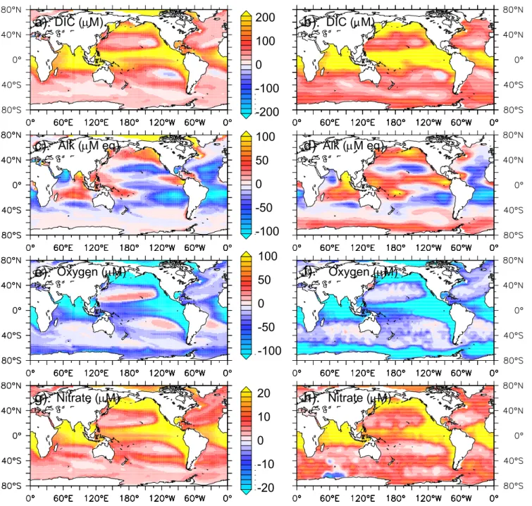
DIC (mM)
a).
c).
e).
g).
b).
d)
f).
h).
200
100
0
-100
-200
100
50
0
-50
-100
DIC (mM)
Alk (mM eq)
Alk (mM eq)
Oxygen (mM)
100
50
0
-50
-100
Oxygen (mM)
Nitrate (mM)
20
10
0
-10
-20
Nitrate (mM)
FIGURE 3 (1)
Fig. 3. The gradient (between 200 m and the surface) simulated by PISCES in dissolved inorganic carbon (a DIC, µM), alkalinity (c ALK, µM eq), oxygen (e O2, µM), nitrates (f NO3, µM), iron (i Fe, nM), nitrous oxide (j N2O, nM), dimethylsulfide (k DMS, nM). When available, is also displayed the same gradient from observation-based climatologies: GLODAP for DIC (b) and alkalinity (d), World Ocean Atlas for oxygen (f) and nitrates (h).biological productivity and export of carbon (Fig. 2). The enhancement of export can be as great as 450 g C m−2yr−1, or as low as 50 g C m−2yr−1in the equatorial Pacific and Southern Oceans (Fig. 2). In addition, non-local effects as-sociated with the mixing that results from the lateral advec-tion of vertically mixed water are apparent, which are most widespread in the tropical Atlantic, tropical Pacific and In-dian ocean regions.
Contrary to the basic tenet of the pipe hypothesis, phyto-plankton physiological processes act to dampen the impact of the additional nutrient supply on biological productivity in some oceanic regions. In contrast to non Fe limited re-gions, it is evident that the response of export to mixing is very weak in the Fe limited equatorial Pacific and Southern Ocean, in particular (Fig. 2). Two major processes, included in our OGCBM, are responsible for this. First, additional Fe
causes phytoplankton to upregulate their Fe demand (Sunda and Huntsman, 1997), which is very low under the chronic Fe limitation that typically prevails. Second, the additional Fe promotes a shift in species composition towards diatoms (as seen during in situ experiments (de Baar et al., 2005; McAn-drew et al., 2007)), which have a higher demand for Fe than nanophytoplankton. Both physiological and food web pro-cesses act in concert to increase the overall phytoplankton demand for Fe (the Fe/C ratio) and results in a weak “fertil-ization effect” of the additional Fe supplied from mixing.
In contrast to carbon export, the air to sea CO2flux (FCO2)
declines markedly at the site of all pipes (Fig. 2). Evidently the impact of mixing surface waters with carbon rich deep waters is greater than the additional CO2drawdown
associ-ated with the increased biological productivity. Parallel to that seen for carbon export, we also note non-local effects on FCO2, which are generally positive (i.e., increased ocean
uptake of CO2)at high latitudes and negative (i.e., reduced
ocean uptake of CO2)in the tropics (Fig. 2). These patterns
could be driven by either increased biological drawdown of CO2, or alkalinity anomalies in the surrounding regions.
3.2.2 Quantifying the mechanisms that control FCO2
Three main mechanisms control the impact of ocean pipes on
pCO2and thus FCO2. Firstly, the profile of DIC increases
with depth (Fig. 3) and accordingly, increased mixing brings carbon rich deep water to the surface, which increases pCO2
and reduces FCO2. Secondly, the fertilization of
biologi-cal productivity increases the consumption of DIC during photosynthesis, which reduces pCO2 and increases FCO2.
Thirdly, the spatial variability of the alkalinity profile (which can be either positive or negative, Fig. 3) can either reduce or increase pCO2, depending on whether more, or less,
alkalin-ity is provided to surface waters. All three mechanisms (DIC, biological production and alkalinity) will control the ultimate impact of mixing on pCO2in a given oceanic region.
In Table 1, we quantify the impact of changes in DIC mix-ing, biological production and alkalinity (all in µmol kg−1)
on pCO2(in ppm) at both the pipe location and the
surround-ing waters. We focus on three particular regions that high-light the interplay between the three controlling processes in governing the eventual impact on FCO2.
We first focus on the area surrounding a given pipe to ac-count for lateral advection. In the tropical Atlantic, DIC mix-ing increases pCO2 by 10 ppm, but biological productivity
responds greatly to the increased mixing and lowers pCO2
by approximately 5ppm. Since tropical regions have a nega-tive alkalinity profile (Fig. 3), mixing also reduces surface alkalinity by 3 µmol kg−1 and pCO2 increases by 4 ppm.
Therefore, the net impact of mixing in the tropical Atlantic is to increase surface pCO2 by 9.6 ppm and reduce FCO2.
In the Southern Ocean we have already noted that mixing only results in a weak biological response (0.17 µmol kg−1)
that lowers pCO2 by 0.5 ppm. However, as this region is
FIGURE 3 (2)
Fe (nM)i).
1 0.5 0 -0.5 -1 N2O (nM)j).
40 20 0 -20 -40 DMS (nM)k).
4 2 0 -4 -2 Fig. 3. Continued.characterized by a weakly positive alkalinity profile (Fig. 3), the small increase in surface alkalinity lowers pCO2 by a
further 3 ppm. Nevertheless, the greater supply of DIC con-tributes ∼7 ppm to pCO2and the net result is a 3.3 ppm
in-crease and lesser FCO2. In the sub-Arctic Pacific, we find a
moderately strong biological contribution to lowering pCO2
(−2.9 ppm) and the strongly positive alkalinity profile re-sults in a large alkalinity increase (4 µmol kg−1)that reduces pCO2by another 9.7 ppm. This increase in alkalinity means
that, although extra vertical supply of DIC increases pCO2
by 12 ppm, the net effect of mixing is to slightly lower pCO2
in this region and create a sink for atmospheric CO2 (by
0.6 ppm). The regional heterogeneity present in the alkalinity gradient means that as the alkalinity anomaly advects later-ally into the surrounding waters FCO2 increases in regions
where the gradient is positive and declines where the gradi-ent is negative (Figs. 2, 3).
If we now only examine the results at the precise pipe lo-cation, two major observations can be made. Firstly, unsur-prisingly, it is clear that for all 3 processes (DIC, alkalinity and biological production) the effect is far greater at the pipe site than when evaluated over the surrounding waters (Ta-ble 1). However, it is noteworthy that the “enhancement”
Table 1. The individual impact of changes in DIC, alkalinity, and biological export on pCO2(in ppm), as well as the eventual 1pCO2 (ppm), over the surrounding waters (see Methods) for three characteristic regions (the result at the pipe location is in parentheses).
Individual impact on pCO2(ppm)
Overall 1pCO2(ppm) DIC Alkalinity Export
Sub-Arctic Pacific +12 (+284) −9.7 (−69) −2.9 (−19.5) −0.6 (+195.5) Tropical Atlantic +8.6 (+95.8) +4.0 (+17.9) −5.0 (−15.1) +9.6 (+98.6) Southern Ocean +6.8 (+39.2) −3.0 (−11.4) −0.5 (−2.0) +3.3 (+25.8) -0.2 -0.1 0 0.1 0.2 2000 2002 2004 2006 2008 2010 2012 2014 2016 2018 20200 0.02 0.04 0.06 0.08 0.1 FCO2 FN2O FDMS CEX Year P ro po rti on al c ha ng e in F C O2 a nd F N2 O Pro po rtio na l c ha ng e in F D M S a nd C ex
FIGURE 4
Fig. 4. The temporal evolution of the proportional difference in
carbon export (Cex), and air to sea fluxes of CO2(FCO2), DMS (FDMS), and N2O (FN2O) from 2000 and 2020 in response to our patchy mixing experiment. Proportional changes in FCO2and FN2O are on the left hand y-axis, and the proportional changes in Cex and FDMS are on the right hand y-axis.
at the site of mixing is far greater for DIC than for alkalinity and biological production (Table 1). It appears that most DIC outgases to the atmosphere where mixing occurs, whereas al-kalinity and nutrient anomalies are able advect into the sur-rounding waters. Accordingly, mixing is only ever beneficial (in terms of FCO2)because of the proximal consequences (i.e., biological production and greater alkalinity).
Overall, our analysis demonstrates that the enhancement of biological productivity is never enough to compensate for the additional supply of DIC to surface waters. It is only if sufficient alkalinity can also be added to surface waters that the effect of artificial mixing is to lower pCO2. If the
addi-tion of alkalinity occurs alongside a strong increase in carbon export, then the decrease in pCO2will be maximal. Only the
Southern Ocean and the sub-Arctic Pacific have the requisite non-negative alkalinity profile (Table 1, Fig. 3). Of these, only in the sub-Arctic Pacific is enough additional alkalinity provided to lower pCO2and create an atmospheric CO2sink
(Table 1).
3.2.3 Impact of mixing on atmospheric CO2, DMS and
N2O
Unsurprisingly, we find that deploying an array of ocean pipes acts to increase atmospheric CO2 by 1.4 ppm via a
5.1% reduction in cumulative FCO2, despite augmenting
car-bon export by 5.6%. This is contrary to the expectations of Lovelock and Rapley (2007) and results from increased mix-ing with sub-surface DIC-rich waters (Table 1, as noted by Shepherd et al., 2007), which overwhelms any beneficial re-sponse due to increased export and alkalinity supply. The positive anomalies in biological productivity and carbon ex-port are maximal over the first few years of the experiment and decay by 20–30% after 20 years of deployment (Fig. 4). We further note that if we eliminate the non-local effects and mix the entire global ocean then while carbon export is over 50% greater, atmospheric CO2 increases by over 20 ppm.
Accordingly, carbon export and FCO2are clearly decoupled
in response to changes in ocean mixing.
We can produce a net global ocean carbon sink if we re-strict the artificial mixing to the sub-Arctic Pacific (see Meth-ods), which was the only region where we found mixing to reduce surface ocean pCO2 (Table 1). However, while we
do find net uptake of atmospheric CO2, this only contributes
one tenth of a ppm (−0.11 ppm, or −3×10⁻¹⁵ppm m−2
when area-normalized) to atmospheric CO2 over 20 years.
It therefore appears that even mixing favorable regions is not a very efficient way to significantly lower atmospheric CO2.
For context, regional mixing experiments in the equatorial Pacific and Southern Oceans (see Methods) increase atmo-spheric pCO2by 9×10−14 and 7×10⁻¹⁴ppm m−2(or 0.76
and 4.15 ppm in total), respectively.
Ocean to atmosphere fluxes of DMS are increased in re-sponse to greater ocean mixing (Fig. 4). The enhancement of biological productivity causes greater production of DMS (Fig. 3), although this is somewhat reduced by the elevated diatom abundance (which produce less DMS than nanophy-toplankton, (Bopp et al., 2008)) and results in a 7.7% in-crease in the globally integrated cumulative DMS flux to the atmosphere over 20 years. In the Southern Ocean and equatorial Pacific, the small increase in biologically medi-ated DMS production (see above) means that the vertical sup-ply of DMS-poor subsurface water (Fig. 3) causes surface
concentrations of DMS, and hence also ocean to atmosphere fluxes, to decline (Fig. 2). Overall, the temporal evolutions of the anomalies in the DMS flux track those of biological activ-ity, which is the dominant source term for DMS. During sim-ulations of Fe fertilization experiments, Bopp et al. (2008) found that despite a large increase in primary production, ad-ditional biological effects associated with the Fe fertilization (i.e., increased bacterial consumption, reduced phytoplank-ton S/C ratio, and reduced DMSP to DMS transfer efficiency) resulted in no increase in DMS. In this study, such processes also occur and dampen the effect of increased biological ac-tivity on DMS flux to the atmosphere.
The increased O2 consumption during the
remineralisa-tion of the greater quantities of organic carbon exported to depth increases the production of the climatically important gas N2O. Indeed, the 20 year cumulative N2O flux to the
at-mosphere increases (Figs. 2, 4) by 4.5% in response to mix-ing when globally integrated, which would increase radiative forcing. However, the global N2O flux exhibits a sharp
de-cline following its initial peak and the flux anomaly reaches near zero by 2020 (Fig. 4). This is due to both an increase in the atmospheric N2O concentration that retards the air-sea
gradient and an O2-driven reduction in the N2O source term
in the ocean. Elevated vertical mixing drives greater mixing of high O2surface waters with O2poor subsurface (Fig. 3),
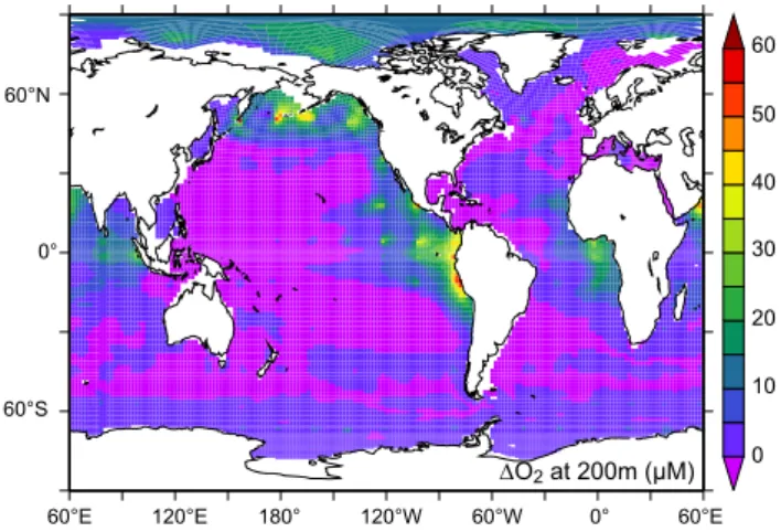
which increases O2concentrations (Fig. 5), especially in
re-gions typified by high N2O fluxes (Fig. 1c). Greater
concen-trations of O2reduce in situ denitrification rates and hence
also the “low oxygen” pathway for the production of N2O.
Over decadal timescales, the increased subsurface oxygen associated with greater degrees of vertical mixing has the potential to reduce ocean sources of N2O, despite an
in-creased source in the short term (i.e., 20 years, Fig. 4). Ad-ditionally, under elevated vertical mixing, the greater subsur-face concentrations of NO3 resulting from reduced
denitri-fication will be efficiently transported to surface waters and drive reductions in surface water N2fixation (Tagliabue et al.,
2008). Although the oceanic N2O source might decline over
multi-decadal timescales (especially in the equatorial Pacific, Fig. 2), it is accompanied by increasing concentrations of at-mospheric CO2.
4 Limitations of our approach
Our study required us to simplify how we represented ocean pipes in our OGCBM. In particular, the model grid size (see Methods section) is obviously far greater than the proposed 10 m diameter pipes and our approach of extending the max-imum vertical diffusivity to 200 m does not precisely repre-sent the pumping of water from 200 m to the surface. How-ever, we believe our resolution is sufficient to be able to de-scribe and quantify the non-local effects associated with a pipe. In addition, our representation of the pumping of nutri-ents and other tracers, while not a direct analogue, represnutri-ents
the first order impact of such a process (bringing subsurface waters to the surface).
Since our OGCBM was run offline, we do not represent the impact of enhanced mixing on the profile of temperature or changes in the density structure of the newly mixed water column. Deeper waters are typically colder than those at the surface and therefore one would anticipate mixing to cool the surface waters, increasing the solubility of CO2 and
reduc-ing pCO2. On the other hand, supplying denser subsurface
water to the surface, where it would overly less dense wa-ter, would destabilize and possibly further deepen the mixed layer (Lampitt et al., 2008). As we have shown, this would act to increase light limitation of photosynthesis, as well as its Fe demand (expressed as an increase in both chlorophyll and Fe to carbon ratios) and lower biological productivity.
PISCES is a relatively complex OGCBM in terms of the biological processes accounted for. As such, there are cer-tain parameters that are necessarily unconstrained. Although we did not perform an exhaustive sensitivity analysis during this particular study, the analysis in Table 1 shows that the predominant drivers of the pCO2response are DIC and
al-kalinity initial concentrations which are independent of the response of the biological activity to enhanced mixing.
In addition, although PISCES is a relatively complex OGCBM, it does not represent variability in C/N/P ratios during the production and remineralisation of organic matter. Any resulting C/N/P variability might therefore be important in governing the CO2response to enhanced vertical mixing
in oligotrophic regions that are limited by N and P. That said, variability in C/N/P demands arise from complex cel-lular processes and adaptation (e.g., Klausmeier et al., 2004) and their inclusion in a global 3-D OGCBM is not straight-forward at this stage. On the other hand, PISCES does rep-resent variability in Fe/C ratios (as observed by laboratory studies, e.g., Sunda and Huntsman, 1997). Accounting for this phytoplankton physiological response results in a weak export response to the increased Fe concentrations (arising from enhanced mixing) in the Southern Ocean. Finally, we also note that as more similar studies are performed using alternative OGCBMs, we will be in a position to better es-timate the overall uncertainty associated with the particular modeling strategies adopted.
Since our OGCBM is not directly coupled to the climate, the role of changes in climate induced by the increased ocean outgassing of CO2, DMS, and N2O is not accounted for. For
example, changes in the quantities of CO2, DMS, and N2O
will impact the atmospheric heat balance and its associated dynamics, which will feedback on the ocean dynamics via modified precipitation, heat fluxes, and winds. We do, how-ever, account for changes in flux when accounting for the concentration of atmospheric gases during the gas flux cal-culations (see Methods).
0 10 20 30 40 50 60 DO2 at 200m (µM) 60°E 60°S 0° 60°N 120°E 180° 120°W 60°W 0° 60°E
FIGURE 5
Fig. 5. The change in O2concentration (µM) at 200 m in 2020 in response to our patchy mixing experiment.5 Perspectives
While it appears that (considering the limitations of our ap-proach) an artificial enhancement of ocean mixing does not show great potential as a means by which we can lower atmo-spheric CO2 levels, our results are also important in
under-standing the impact of natural variability in mixing on FCO2.
For example, Le Qu´er´e et al. (2007) noted a weakening of Southern Ocean FCO2(by 0.08 Pg C yr−1), associated with
increased wind driven ventilation of carbon rich deep waters. Our analyses show that the impact of enhanced mixing on Southern Ocean FCO2is dominated by the increased surface
DIC concentrations associated with greater vertical mixing and that compensatory feedbacks (in terms of pCO2)by al-kalinity and biology are relatively weak (Table 1). For ex-ample, if we mix the region 40◦S to 60◦S to 200 m for 20
years, then atmospheric pCO2 increases by 4.2 ppm.
Trop-ical regions, in particular, appear very vulnerable to mixing induced increases in surface pCO2as, despite a more
favor-able productivity response, the local alkalinity profile (lower in the subsurface, Fig. 3) exacerbates the DIC driven increase in pCO2. It is for this reason that large scale upwelling
sys-tems (such as that off the coast of Peru) are typically large sources of CO2 to the atmosphere (Takahashi et al., 2008,
Fig. 1). On the other hand, the strongly positive alkalinity profile in the sub-Arctic Pacific (Fig. 2) means that the in-creased alkalinity associated with inin-creased mixing can po-tentially compensate for the increased pCO2due to DIC
in-creases. Accordingly, FCO2is most vulnerable to changes in
mixing in the tropics, followed by the Southern Ocean, while in sub-Arctic Pacific FCO2is much less sensitive to mixing
(as demonstrated by our regional mixing experiments).
6 Conclusions
We included a representation of ocean pipes that mechani-cally augment ocean mixing in an OGCBM to address their potential impact on carbon export and CO2 fluxes. We
find that despite increasing carbon export markedly, ocean to atmosphere CO2fluxes increase and atmospheric CO2is
greater by 2020. The increased vertical supply of carbon rich deep water is primarily responsible for the enhanced out-gassing, although increased alkalinity can compensate in the northern Pacific Ocean. Physiological processes and shifts in ecosystem composition temper the biological response in Fe limited regions such as the Southern Ocean. Even if we focus on a region where mixing is favorable, we can only create a very weak carbon sink that is not an efficient control on atmospheric CO2. While fluxes of DMS to the
atmosphere do increase slightly, which might promote the formation of cloud condensation nuclei, the oceanic N2O
source also expands, which would increase radiative heat-ing of the atmosphere (alongside the increased atmospheric CO2). Aside from demonstrating that pipes have a limited
geo-engineering potential, our study demonstrates how nat-ural variability in mixing (such as that observed recently in the Southern Ocean) can impact pCO2and hence FCO2 in
the global ocean.
Acknowledgements. Simulations were performed at CNRS/IDRIS
and CEA/CCRT, France. We thank Olivier Aumont, Sauveur Belviso, Patricia Cadule, and Corinne Le Qu´er´e for their ideas and comments, Cynthia Nevison for providing the N2O flux database and Taro Takahashi for providing the ocean 1pCO2 database. This study was begun during the stay of L.B. at the University of East Anglia (UK) with the support of NERC/QUEST. Edited by: C. Slomp
The publication of this article is financed by CNRS-INSU.
References
Arrigo, K. R. and Tagliabue, A.: Iron in the Ross Sea, Part II: Im-pact of discrete iron addition strategies, J. Geophys. Res., 110, C03010, doi:10.1029/2004JC002568, 2005.
Aumont, O. and Bopp, L.: Globalizing results from ocean in situ iron fertilization studies, Global Biogeochem. Cycles, 20, GB2017, doi:10.1029/2005GB002591, 2006.
Belviso, S., Bopp, L., Moulin, C., Orr, J. C., Anderson, T. R., Chu, S., Elliott, S., Maltrud, M. E., and Simo, R.: Comparison of global climatological maps of sea surface dimethylsulfide, Global Biogeochem. Cycles, 18, GB3013, doi:10.1029GB2003002193, 2004.
Bopp, L., Aumont, O., Belviso, S., and Blain, S.: Modelling the effect of iron fertilization on dimethylsulphide emissions in the Southern Ocean, Deep-Sea Res. Part II, 55, 901–912, 2008. Boyd, P. W., Jickells, T., Law, C. S., et al.: Mesoscale iron
enrich-ment experienrich-ments 1993–2005: Synthesis and future directions, Science, 315(5812), 612–617, 2007.
Boyd, P. W., Watson, A. J., Law, C. S., Abraham, E. R., Trull, T., Murdoch, R., Bakker, D. C. E., Bowie, A. R., Buesseler, K. O., Chang, H., and Charette, M.: A mesoscale phytoplankton bloom in the polar Southern Ocean stimulated by iron fertilization, Na-ture, 407, 695–702, 2000.
Carr, M.-E., Friedrichs, M. A. M., Schmeltz, M., et al.: A compari-son of global estimates of marine primary production from ocean color, Deep-Sea Res. Part II, 53, 741–770, 2006.
Chu, S., Elliott, S., and Maltrud, M. E.: Global eddy permitting sim-ulations of surface ocean nitrogen, iron, sulfur cycling, Chemo-sphere, 50, 223–235, 2003.
Cullen, J. J. and Boyd, P. W.: Predicting and verifying the intended and unintended consequences of large-scale ocean iron fertiliza-tion, Mar. Ecol. Prog. Ser., 364, 295–301, 2008.
de Baar, H. J. W., Boyd, P. W., Coale, K. H., et al: Synthe-sis of iron fertilization experiments: From the iron age in the age of enlightenment, J. Geophys. Res., 110, C09S16, doi:10.1029/2004JC002601, 2005.
Denman, K. L., Brasseur, G., Chidthaisong, A., Ciais, P., Cox, P., Dickinson, R. E., Haugustaine, D., Heinze, C., Holland, E., Ja-cob, D., Lohmann, U., Ramachandran, S., da Silva Dias, P. L., Wofsy, S. C., and Zhang, X.: Couplings Between Changes in the Climate System and Biogeochemistry, p. 499–587, in: Cli-mate Change 2007: The Physical Science Basis. Contribution of Working Group I to the Fourth Assessment Report of the Inter-governmental Panel on Climate Change, edited by: Solomon, S., Qin, D., Manning, M., Chen, Z., Marquis, M., Averyt, K. B., Tignor, M., and Miller, H. L., Cambridge University Press, Cam-bridge, United Kingdom and New York, NY, USA, 2007. Dufresne, J. L., Friedlingstein, P., Berthelot, M., Bopp, L., Ciais,
P., Fairhead, L., LeTreut, H., and Monfray, P.: Effects of climate change due to CO2 increase on land and ocean carbon uptake, Geophys. Res. Lett., 29(10), 1405, doi:10.1029/2001GL013777, 2002.
Fichefet, T. and Morales Maqueda, M. A.: Sensitivity of a global sea ice model to the treatment of ice thermodynamics and dy-namics, J. Geophys. Res., 102, 12609–12646, 1997.
Fennel, K.: Widespread implementation of controlled upwelling in the North Pacific Subtropical Gyre would counteract dia-zotrophic N2 fixation, Mar. Ecol. Prog. Ser., 371, 301–303, 2008. Karl, D. M. and Letelier, R. M.: Nitrogen fixation-enhanced car-bon sequestration in low nitrate, low chlorophyll seascapes, Mar. Ecol. Prog. Ser., 364, 257–268, 2008.
Kettle, A. J. and Andreae, M. O.: Flux of dimethylsulfide from the oceans: A comparison of updated data sets and flux models, J. Geophys. Res., 105, 26793–26808, 2000.
Klausmeier, C. A., Litchman, E., Daufresne, T., and Levin, S. A.: Optimal N:P stoichiometry of phytoplankton, Nature, 429, 171– 174, 2004.
Jin, X. and Gruber, N.: Offsetting the radiative benefit of ocean iron fertilization by enhancing N2O emissions, Geophys. Res. Lett., 30, 2249, doi:10.1029/2003GL018458, 2003.
Lampitt, R. S., Achterberg, E. P., Anderson, T. R., Hughes, J. A.,
Iglesias-Rodriguez, M. D., Kelly-Gerreyn, B. A., Lucas, M., Popova, E. E., Sanders, R., Shepherd, J. G., Smythe-Wright, D., and Yool, A.: Ocean fertilization: a potential means of geoengi-neering?, Philos. T. R. Soc. A, 366(1882), 3919–3945, 2008. Leinen, M.: Building relationships between scientists and business
in ocean iron fertilization, Mar. Ecol. Prog. Ser., 364, 251–256, 2008.
Le Qu´er´e, C., R¨odenbeck, C., Buitenhuis, E. T., Conway, T. J., Langenfelds, R., Gomez, A., Labuschagne, C., Ramonet, M., Nakazawa, T., Metzl, N., Gillett, N., and Heimann, M.: Satura-tion of the Soutner Ocean CO2 sink due to recent climate change, Science, 316, 1735–1738, doi:10.1126/science.1136188, 2007. Lovelock, J. E. and Rapley, C. G.: Ocean pipes could help the Earth
to cure itself, Nature, 449–403, 2007.
McAndrew, P. M., Bjorkman, K. M., Church, M. J., Morris, P. J., Ja-chowski, N., Williams, P. J., and Karl, D. M.: Metabolic response of oligotrophic plankton communities to deep water nutrient en-richment, Mar. Ecol. Prog. Ser., 332, 63–75, 2007.
Madec, G., Delecluse, P., Imbard, M., and Levy, C.: OPA8.1 Ocean General Circulation Model Reference Manual, Notes du pˆole de mod´elisation de l’IPSL, 1998.
Markels Jr., M. and Barber, R. T.: Sequestration of carbon dioxide by ocean fertilization. Paper presented at the 1st Nat Conf on Car-bon Sequestration, Natl Energy Technol Lab, Washington, D.C., 14–17 May 2001.
Nakisenovic, N., Alcamo, J., Davis, G., et al.: IPCC Special Re-port on Emissions Scenarios, Cambridge Univ. Press, New York, 2000.
Nevison, C. D., Weiss, R. F., and Erickson, D. J.: Global oceanic emissions of nitrous oxide, J. Geophys. Res., 100, 15809–15820, 1995.
Raven, J. A.: The iron and molybdenum use efficiencies of plant growth with different energy, carbon and nitrogen sources, New Phytol., 109, 279–287, 1988.
Saltzman, E. S., King, D. B., Holmen, K., and Leck, C.: Experi-mental determination of the diffusion coefficient of dimethylsul-fide in water, J. Geophys. Res., 98, 16481–16486, 1993. Schlitzer, R.: Applying the adjoint method for biogeochemical
modeling: Export of particulate organic matter in the World Ocean, Inverse methods in biogeochemical cycles, edited by: Kasibhata, P., AGU Monograph, 114, 107–124, 2000.
Sciare, J., Mihalopoulos, N., and Dentener, F.: Interannual variabil-ity of atmospheric dimethylsulfide in the southern indian ocean, J. Geophys. Res., 105, 26369–26377, 2000.
Shepherd, J. G., Inglesias-Rodriguez, D., and Yool, A.: Geo-engineering might cause, not cure, problems, Nature, 449, 781, 2007.
Sim´o, R. and Dachs, J.: Global ocean emission of dimethylsulfide predicted from biogeophysical data, Global Biogeochem. Cy-cles, 16(4), 1078, doi:10.1029/2001GB001829, 2007.
Sunda, W. G. and Huntsman, S. A.: Interrelated influence of iron, light and cell size on marine phytoplankton growth, Nature, 390, 389–392, 1997.
Suntharalingam, P., Sarmiento, J. L., and Toggweiler, J. R.: Global significance of nitrous-oxide production and transport from oceanic low-oxygen zones: A modeling study, Global Bio-geochem. Cycles, 14, 1353–1370, 2000.
Takahashi, T., Sutherland, S. C., Wanninkhof, R., et al.: Cli-matological mean surface pCO2 and net CO2 flux over
the global oceans, Deep Sea Res. Part II, published online, doi:10.1016/j.dsr2.2008.12.009, 2008.
Tagliabue, A., Bopp, L., and Aumont, O.: Ocean biogeochemistry exhibits contrasting responses to a large scale reduction in dust deposition, Biogeosciences, 5, 11–24, 2008,
http://www.biogeosciences.net/5/11/2008/.
Volk, T. and Hoffert, M. I.: Ocean carbon pumps: analysis of rela-tive strengths and efficiencies in ocean-driven atmospheric CO2 changes, in: The Carbon Cycle and Atmospheric CO2: Natu-ral Variations Archean to Present, edited by: Sundquist, E. T. and Broecker, W. S., pp. 99–110, Geophysical Monograph 32, American Geophysical Union, Wash., D.C., 1985.
Wanninkhof, R.: Relationship between wind speed and gas ex-change over the ocean, J. Geophys. Res., 97, 7373–7382, 1992. Zeebe, R. E. and Wolf-Gladrow, D.: CO2in seawater: equilibrium,