HAL Id: hal-02369296
https://hal.inria.fr/hal-02369296
Submitted on 18 Nov 2019
HAL is a multi-disciplinary open access archive for the deposit and dissemination of sci-entific research documents, whether they are pub-lished or not. The documents may come from teaching and research institutions in France or abroad, or from public or private research centers.
L’archive ouverte pluridisciplinaire HAL, est destinée au dépôt et à la diffusion de documents scientifiques de niveau recherche, publiés ou non, émanant des établissements d’enseignement et de recherche français ou étrangers, des laboratoires publics ou privés.
Amit Jaiswal, Jukka Nenonen, Matti Stenroos, Alexandre Gramfort, Sarang
Dalal, Britta Westner, Vladimir Litvak, John Mosher, Jan-Mathijs Schoffelen,
Caroline Witton, et al.
To cite this version:
Amit Jaiswal, Jukka Nenonen, Matti Stenroos, Alexandre Gramfort, Sarang Dalal, et al..
Com-parison of beamformer implementations for MEG source localization. NeuroImage, 2020, 216,
1
Comparison of beamformer implementations for MEG source
1
localization
2
Amit Jaiswal1,2, Jukka Nenonen1, Matti Stenroos2, Alexandre Gramfort3, Sarang S. Dalal4, Britta U. Westner4,
3
Vladimir Litvak5, John C. Mosher6, Jan-Mathijs Schoffelen7, Caroline Witton9,Robert Oostenveld7,8, Lauri
4
Parkkonen1,2
5
1Megin Oy1, Helsinki, Finland.
6
2Department of Neuroscience and Biomedical Engineering, Aalto University School of Science, Espoo, Finland
7
3Inria, CEA/Neurospin, Universite Paris-Saclay, Paris, France
8
4Center of Functionally Integrative Neuroscience, Aarhus University, Denmark
9
5The Wellcome Centre for Human Neuroimaging, UCL Queen Square Institute of Neurology, London, UK
10
6Department of Neurology, University of Texas Health Science Center at Houston, Houston, Texas, USA
11
7Donders Institute for Brain, Cognition and Behaviour, Radboud University, Nijmegen, The Netherlands
12
8NatMEG, Karolinska Institutet, Stockholm, Sweden
13
9Aston Brain Centre, School of Life and Health Sciences, Aston University, Birmingham, UK
14
_______________________________________________________________________
15
Abstract
16
Beamformers are applied for estimating spatiotemporal characteristics of neuronal sources 17
underlying measured MEG/EEG signals. Several MEG analysis toolboxes include an 18
implementation of a linearly constrained minimum-variance (LCMV) beamformer. However, 19
differences in implementations and in their results complicate the selection and application of 20
beamformers and may hinder their wider adoption in research and clinical use. Additionally, 21
combinations of different MEG sensor types (such as magnetometers and planar gradiometers) and 22
application of preprocessing methods for interference suppression, such as signal space separation 23
(SSS), can affect the results in different ways for different implementations. So far, a systematic 24
evaluation of the different implementations has not been performed. Here, we compared the 25
localization performance of the LCMV beamformer pipelines in four widely used open-source 26
toolboxes (FieldTrip, SPM12, Brainstorm, and MNE-Python) using datasets both with and without
27
SSS interference suppression. 28
We analyzed MEG data that were i) simulated, ii) recorded from a static and moving phantom, and 29
iii) recorded from a healthy volunteer receiving auditory, visual, and somatosensory stimulation. We 30
also investigated the effects of SSS and the combination of the magnetometer and gradiometer 31
signals. We quantified how localization error and point-spread volume vary with SNR in all four 32
toolboxes. 33
2
When applied carefully to MEG data with a typical SNR (3–15 dB), all four toolboxes localized the 34
sources reliably; however, they differed in their sensitivity to preprocessing parameters. As expected, 35
localizations were highly unreliable at very low SNR, but we found high localization error also at very 36
high SNRs. We also found that the SNR improvement offered by SSS led to more accurate 37
localization. 38
Keywords
39
MEG, EEG, source modeling, beamformers, LCMV, open-source analysis toolbox. 40
41 42
3
1. Introduction
43
MEG (magnetoencephalography) and EEG (electroencephalography) source imaging aims to 44
identify the spatiotemporal characteristics of neural source currents based on the recorded signals, 45
electromagnetic forward models and physiologically motivated assumptions about the source 46
distribution. One well-known method for estimating a small number of focal sources is to model each 47
of them as a current dipole with fixed location and fixed or changing orientation. The locations 48
(optionally orientations) and time courses of the dipoles are then collectively estimated (Mosher et 49
al., 1992; Hämäläinen et al., 1993). Such equivalent dipole models have been widely applied in basic 50
research (see e.g. Salmelin, 2010) as well as in clinical practice (Bagic et al., 2011a; 2011b; Burgess 51
et al., 2011). Distributed source imaging estimates source currents distribution across the whole 52
source space, typically the cortical surface. Examples of linear methods for distributed source 53
estimation are LORETA (low-resolution brain electromagnetic tomography; Pascual-Marqui et al., 54
1994) and MNE (minimum-norm estimation; Hämäläinen and Ilmoniemi, 1994). From estimated 55
source distributions, one often computes noise-normalized estimates such as dSPM (dynamic 56
statistical parametric mapping; Dale et al., 2000). Also, various non-linear distributed inverse 57
methods have been proposed (Wipf et al., 2010; Gramfort et al., 2013b). 58
While dipole modeling and distributed source imaging estimate source distributions that reconstruct 59
(the relevant part of) the measurement, beamforming takes an adaptive spatial-filtering approach, 60
scanning independently each location in a predefined region of interest (ROI) within the source space 61
without attempting to reconstruct the data. Beamforming can be done in time-or frequency domain; 62
time-domain methods are typically based on the LCMV approach (Van Veen and Buckley, 1988; 63
1997; Spencer et al., 1992; Sekihara et al., 2006), and in frequency domain the DICS (Dynamic 64
Imaging of Coherent Sources) (Gross et al., 2001) approach is popular. 65
The LCMV beamformer estimates the activity for a source at a given location (typically a point 66
source) while simultaneously suppressing the contributions from all other sources and noise 67
captured in the data covariance matrix. For evaluation of the spatial distribution of the estimated 68
source activity, an image is formed by scanning a set of predefined possible source locations and 69
computing the beamformer output (often power) at each location in the scanning space. When the 70
scanning is done in a volume grid, the beamformer output is typically presented by superimposing it 71
onto an anatomical MRI. 72
Beamformers have been popular in basic MEG research studies (e.g. Hillebrand and Barnes, 2005;
73
Braca et al., 2011; Ishii et al., 2014; van Es and Schoffelen, 2019) as well as in clinical applications 74
such as in localization of epileptic events (e.g. Van Klink et al., 2017; Youssofzadeh et al., 2018; Hall 75
et al., 2018). Many variants of beamformers are implemented in several open-source toolboxes and 76
commercial software for MEG/EEG analysis. Presently, based on citation counts, the most used 77
open-source toolboxes for MEG data analysis are FieldTrip (Oostenveld et al., 2011), Brainstorm 78
4
(Tadel et al., 2011), MNE-Python (Gramfort et al., 2013a) and DAiSS in SPM12 (Litvak et al., 2011). 79
These four toolboxes have an implementation of an LCMV beamformer, based on the same 80
theoretical framework (van Veen et al., 1997; Sekihara et al., 2006). Yet, it has been anecdotally 81
reported that these toolboxes may yield different results for the same data. These differences may 82
arise not only from the core of the beamformer implementation but also from the previous steps in 83
the analysis pipeline, including data import, preprocessing, forward model computation, combination 84
of data from different sensor types, covariance estimation, and regularization method. Beamforming 85
results obtained from the same toolbox may also differ substantially depending on the applied 86
preprocessing methods; for example, Signal Space Separation (SSS; Taulu and Kajola 2005) 87
reduces the rank of the data, which could affect beamformer output unpredictably if not appropriately 88
considered in the implementation. 89
In this study, we evaluated the LCMV beamformer pipelines in the four open-source toolboxes and 90
investigated the reasons for possible inconsistencies, which hinder the wider adoption of 91
beamformers to research and clinical use where accurate localization of sources is required, e.g., in 92
pre-surgical evaluation. These issues motivated us to study the conditions in which these toolboxes 93
succeed and fail to provide systematic results for the same data and to investigate the underlying 94
reasons. 95
5
2. Materials and Methods
97
2.1. Datasets
98
To compare the beamformer implementations, we employed MEG data obtained from simulations, 99
phantom measurements, and measurements of a healthy volunteer who received auditory, visual, 100
and somatosensory stimuli. For all human data recordings, informed consent was obtained from all 101
study subjects in agreement with the approval of the local ethics committee. 102
2.1.1. MEG systems
103
All MEG recordings were performed in a magnetically shielded room with a 306-channel MEG 104
system (either Elekta Neuromag® VectorView or TRIUXTM; Megin Oy, Helsinki, Finland), which
105
samples the magnetic field distribution by 510 coils at distinct locations above the scalp. The coils 106
are configured into 306 independent channels arranged on 102 triple-sensor elements, each housing 107
a magnetometer and two perpendicular planar gradiometers. The location of the phantom or 108
subject’s head relative to the MEG sensor array was determined using four or five head position 109
indicator (HPI) coils attached to the scalp. A Polhemus Fastrak®system (Colchester, VT, USA) was 110
used for digitizing three anatomical landmarks (nasion, left and right preauricular points) to define 111
the head coordinate system. Additionally, the centers of the HPI coils and a set of ~50 additional 112
points defining the scalp were also digitized. The head position in the MEG helmet was determined 113
at the beginning of each measurement using the ‘single-shot’ HPI procedure, where the coils are 114
activated briefly, and the coil positions are estimated from the measured signals. The location and 115
orientation of the head with respect to the helmet can then be calculated since the coil locations were 116
known both in the head and in the device coordinate systems. After this initial head position 117
measurement, continuous tracking of head movements (cHPI) was engaged by keeping the HPI 118
coils activated to track the movement continuously. 119
2.1.2. Simulated MEG data
120
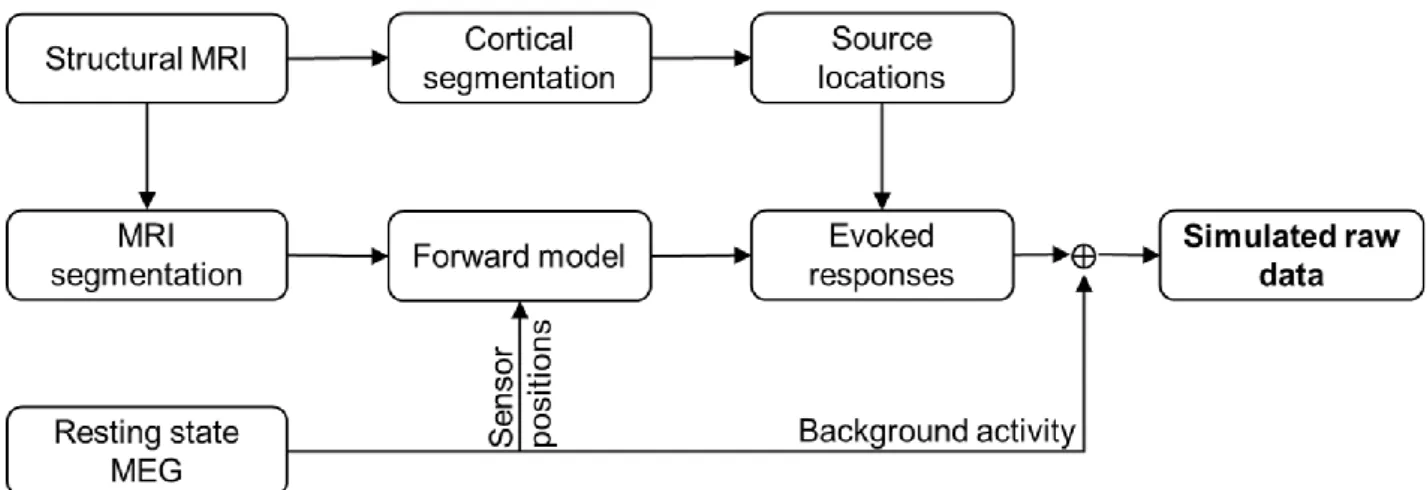
To obtain realistic MEG data with known sources, we superimposed simulated sensor signals based 121
on forward modeling of dipolar sources onto measured spontaneous MEG data utilizing a special in-122
house simulation software. Structural MRI images, acquired from a healthy adult volunteer using a 123
3-tesla MRI scanner (Siemens Trio, Erlangen, Germany), were segmented using the MRI 124
Segmentation Software of Megin Oy (Helsinki, Finland) and the surface enveloping the brain 125
compartment was tessellated with triangles (5-mm side length). Using this mesh, a realistic single-126
shell volume conductor model was constructed using the Boundary Element Method (BEM; 127
Hämäläinen and Sarvas, 1989) implemented in the Source modeling software of Megin Oy. We also 128
segmented the cortical mantle with the FreeSurfer software (Dale et al., 1999; Fischl et al., 1999; 129
Fischl, 2012) for deriving a realistic source space. By using the “ico4” subdivision in MNE-Python, 130
6
we obtained a source space comprising 2560 dipoles (average spacing 6.2 mm) in each hemisphere 131
(Fig. 1). Out of these, we selected 25 roughly uniformly distributed source locations in the left 132
hemisphere for the simulations (Fig. 1). All these points were at least 7.5 mm inwards from the 133
surface of the volume conductor model. We activated each of the 25 dipoles – one at a time – with 134
a 10-Hz sinusoid of 200-ms duration (2 cycles). The dipoles were simulated at eight source 135
amplitudes: 10, 30, 80, 200, 300, 450, 600 and 800 nAm. 136
137
Insert Fig.1 about here 138
139
A continuous resting-state MEG data with eyes open was recorded from the same volunteer who 140
provided the anatomical data, using an Elekta Neuromag® MEG system (at BioMag Laboratory, 141
Helsinki, Finland). The recording length was 2 minutes, the sampling rate was 1 kHz, and the 142
acquisition frequency band was 0.1–330 Hz. This recording provided the head position for the 143
simulations and defined their noise characteristics. MEG and MRI data were co-registered using the 144
digitized head shape points and the outer skin surface in the segmented MRI. 145
The simulated sensor-level evoked fields were superimposed on the unprocessed resting-state 146
recording with inter-trial-interval varying between 1000–1200 ms resulting in ~110 trials (epochs) in 147
each simulated dataset. The resting-state recording was used both as raw without preprocessing 148
and after SSS interference suppression. Altogether, we obtained 400 simulated MEG datasets (25 149
source locations at 8 dipole amplitudes, all both with the raw and SSS-preprocessed real data). Fig. 150
2 illustrates the generation of simulated MEG data. 151
152
Insert Fig. 2 about here 153
2.1.3. Phantom data
154
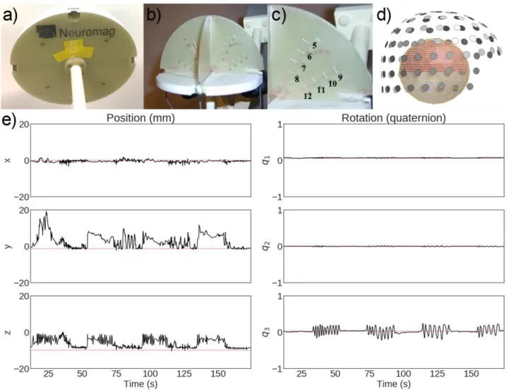
We used a commercial MEG phantom (Megin Oy, Helsinki, Finland) which contains 32 dipoles and 155
4 HPI coils at distinct fixed locations (see Fig 3a–c and Elekta Neuromag® TRIUXTM User’s Manual).
156
The phantom is based on the triangle construction (Ilmoniemi et al., 1985): an isosceles triangular 157
line current generates on its relatively very short side a magnetic field distribution equivalent to that 158
of a tangential current dipole in a spherical conductor model, provided that the vertex of the triangle 159
and the origin of the model of a conducting sphere coincide. The phantom data were recorded from 160
8 dipoles, excited one by one (see Elekta Neuromag® TRIUXTMUser’s Manual), using a 306-channel
161
TRIUXTM system (at Aston University, Birmingham, UK). The distance from the phantom origin was
162
64 mm for dipoles 5 and 9 (the shallowest), 54 mm for dipoles 6 and 10, 44 mm for dipoles 7 and 163
7
11, and 34 mm for dipoles 8 and 12 (the deepest; see Fig 3c). The phantom was first kept stationary 164
inside the MEG helmet and continuous MEG data were recorded with 1-kHz sampling rate for three 165
dipole amplitudes (20, 200 and 1000 nAm); one dipole at a time was excited with a 20-Hz sinusoidal 166
current for 500 ms, followed by 500 ms of inactivity. The recordings were repeated with the 200-nAm 167
dipole strength while moving the phantom continuously to mimic head movements inside the MEG 168
helmet; see the movements in Fig. 3e and Suppl. Fig. 2 for all movement parameters. 169
170
Insert Fig. 3 about here 171
172
2.1.4. Human MEG data
173
We recorded MEG evoked responses from the same volunteer whose MRI and spontaneous MEG 174
data were utilized in the simulations. These human data were recorded using a 306-channel Elekta 175
Neuromag® system (at BioMag Laboratory, Helsinki, Finland). During the MEG acquisition, the 176
subject was receiving a random sequence of visual (a checkerboard pattern in one of the four 177
quadrants of the visual field), somatosensory (electric stimulation of the median nerve at the left/right 178
wrist at the motor threshold) and auditory (1-kHz 50-ms tone pips to the left/right ear) stimuli with an 179
interstimulus interval of ~500 ms. The Presentation software (Neurobehavioral Systems, Inc., 180
Albany, CA, USA) was used to produce the stimuli. 181
2.2. Preprocessing
182
The datasets were analyzed in two ways: 1) omitting bad channels from the analysis, without 183
applying SSS preprocessing, and 2) applying SSS-based preprocessing methods (SSS/tSSS) to 184
reduce magnetic interference and perform movement compensation for moving phantom data. The 185
SSS-based preprocessing and movement compensation were performed in MaxFilterTM software
186
(version 2.2; Megin Oy, Helsinki, Finland). After that, the continuous data were bandpass filtered 187
(passband indicated for each dataset later in the text) followed by the removing the dc. Then the 188
data were epoched to trials around each stimulus. We applied an automatic trial rejection technique 189
based on the maximum variance across all channels, rejecting trials that had variance higher than 190
the 98th percentile of the maximum or lower than the 2nd percentile (see Suppl. Fig. 4). This method
191
is available as an optional preprocessing step in FieldTrip, and the same implementation was applied 192
in the other toolboxes. Below we describe the detailed preprocessing steps for all datasets. 193
2.2.1. Simulated data
194
In each toolbox, the raw data with just bad channels removed or SSS-preprocessed continuous data 195
were filtered using a zero-phase filter with a passband of 2–40 Hz. The filtered data were epoched 196
8
into windows from –200 to +200 ms relative to the start of the source activity. The bad epochs were 197
removed using the variance-based automatic trial rejection technique, resulting in ~100 epochs. 198
Then the noise and data covariance matrices were estimated from these epochs for the time 199
windows of –200 to –20 ms and 20 to 200 ms, respectively. 200
2.2.2. Phantom data
201
All 32 datasets (static: 3 dipole strengths and 8 dipole locations; moving: 1 dipole strength and 8 202
dipole locations) were analyzed both without and with SSS-preprocessing. We applied SSS on static 203
phantom data to remove external interference. On moving-phantom data, combined temporal SSS 204
and movement compensation (tSSS_mc) were applied for suppressing external and movement-205
related interference and for transforming the data from the continuously estimated positions into a 206
static reference position (Taulu and Kajola 2005; Nenonen et al., 2012). Then in each toolbox the 207
continuous data were filtered to 2–40 Hz using a zero-phase bandpass filter, and the filtered data 208
were epoched from –500 to +500 ms with respect to stimulus triggers. Bad epochs were removed 209
using the automated method based on maximum variance, yielding ~100 epochs for each dataset. 210
The noise and data covariance matrices were estimated in each toolbox for the time windows of – 211
500 to –50 ms and 50 to 500 ms, respectively. 212
2.2.3. Human MEG data
213
Both the unprocessed raw data and the data preprocessed with tSSS were filtered to 1–95 Hz using 214
a zero-phase bandpass filter in each toolbox. The trials with somatosensory stimuli (SEF) were 215
epoched between –100 to –10 and 10 to 100 ms for estimating the noise and data covariances, 216
respectively. The corresponding time windows for the auditory-stimulus trials (AEF) were –150 to – 217
20 and 20 to 150 ms, and for the visual stimulus trials (VEF) –200 to –50 and 50 to 200 ms, 218
respectively. Trials contaminated by excessive eye blinks (EOG > 250 μV) or by excessive magnetic 219
signals (MEG > 5000 fT or 3000 fT/cm) were removed with the variance-based automated trial 220
removal technique. Before covariance computation, baseline correction by the time window before 221
the stimulus was applied on each trial. The covariance matrices were estimated independently in 222
each toolbox. 223
Since the actual source locations associated with the evoked fields are not precisely known, we 224
defined reference locations using conventional dipole fitting in the Source Modeling Software of 225
Megin Oy (Helsinki, Finland). A single equivalent dipole was used to represent SEF and VEF 226
sources, and one dipole per hemisphere was used for AEF (see Suppl. Fig. 3). The dipole fitting was 227
performed at the time point of the maximum RMS value across all planar gradiometer channels 228
(global field power) of the average response amplitude. 229
9
2.2.4. Forward model
230
For the beamformer scan of simulated data, we used the default or the most commonly used forward 231
model of each toolbox: a single-compartment BEM model in MNE-Python, a single-shell corrected-232
sphere model (Nolte, 2003) in FieldTrip, a single-shell corrected sphere model (Nolte, 2003) through 233
inverse normalization of template meshes (Mattout et al., 2007) in SPM12(DAiSS), and the 234
overlapping-spheres (Huang et al., 1999) model in Brainstorm. For constructing models for these 235
forward solutions, the segmentation of MRI images was performed in FreeSurfer for MNE-Python 236
and Brainstorm while FieldTrip and SPM12 used the SPM segmentation procedure. A volumetric 237
source space was represented by a rectangular grid with 5-mm resolution and 5-mm minimal 238
distance from the head model surface. Forward solutions were computed separately in each toolbox 239
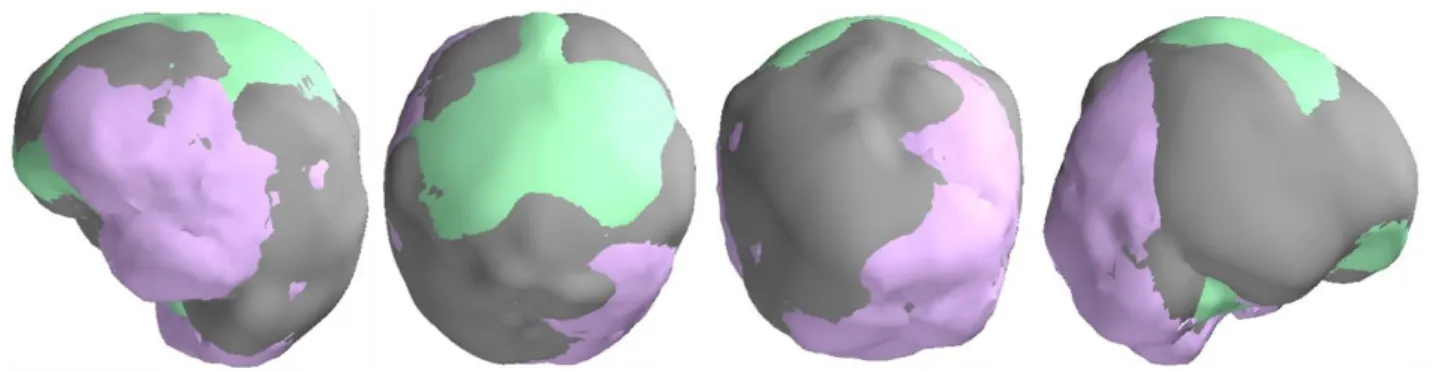
using the head model, the volumetric grid sources, and sensor information from the MEG data. Since 240
each toolbox prepares a head model using a different method, the shape of the head models may 241
slightly differ from each other (see Fig. 4) which further may result in a shift between the positions of 242
the scanning grid in these toolboxes. 243
244
Insert Fig. 4 about here 245
246
For phantom data, a homogeneous spherical volume conductor model was defined in each toolbox 247
with the origin at the head coordinate system origin. An equidistant rectangular source-point grid with 248
5-mm resolution was placed inside the upper half of a sphere covering all 32 dipoles of the phantom; 249
see Fig. 3d. Forward solutions for these grids were computed independently in each toolbox. For 250
human MEG data, the head models and the source space were defined in the same way as for the 251
beamformer scanning of the simulated data. 252
2.3. LCMV beamformer
253
The linearly constrained minimum-variance (LCMV) beamformer is a spatial filter that relates the 254
magnetic field measured outside the head to the underlying neural activities using the covariance of 255
measured signals and models of source activity and signal transfer between the source and the 256
sensor (Spencer et al., 1992; van Veen et al. 1997; Robinson and Vrba, 1998). The spatial filter 257
weights are computed for each location in the region of interest (ROI). 258
Let x be an 𝑀 × 1 signal vector of MEG data measured with 𝑀 sensors, and 𝑁 is the number of grid 259
points in the ROI with grid locations rj, (j = 1, … , 𝑁). Then the source 𝐲(𝑟𝑗) at any location 𝑟𝑗 can be 260
estimated as weighted combination of the measurement x as 261
𝐲(𝑟𝑗) = 𝐖T(𝑟
𝑗)𝐱 (1)
10
where the 𝑀 × 3 matrix 𝐖(𝑟𝑗) is known as spatial filter for a source at location 𝑟𝑗. This type of spatial 263
filter provides a vector type beamformer by separately estimating the activity for three orthogonal 264
source orientations, corresponding to the three columns of the matrix. According to Eqs 16–23 in 265
van Veen et al. (1997), the spatial filter 𝐖(𝑟𝑗) for vector beamformer is defined as 266 𝐖(𝑟𝑗) = (𝐋T(𝑟𝑗)𝐂−1𝐋(𝑟𝑗)) −1 𝐋T(𝑟 𝑗)𝐂−1 (2) 267
Here 𝐋(𝑟𝑗) is the 𝑀 × 3 local leadfield matrix that defines the contribution of a dipole source at location 268
𝑟𝑗 in the measured data x, and 𝐂 is the covariance matrix computed from the measured data samples. 269
To perform source localization using LCMV, the output variance (or output source power) Var(𝐲(rj)) 270
is estimated at each point in the source space (see Eq (24) in van Veen et al., 1997), resulting in 271
Var̂ (𝐲(𝑟𝑗)) = Trace{[𝐋T(𝑟
𝑗)𝐂−1𝐋(𝑟𝑗)]−1} (3)
272
Usually, the measured signal is contaminated by non-uniformly distributed noise and therefore the 273
estimated signal variance is often normalized with projected noise variance 𝐂n calculated over some 274
baseline data (noise). Such normalized estimate is called Neural Activity Index (NAI; van Veen et 275
al., 1997) and can be expressed as 276
NAI(rj) = Trace{[𝐋T(𝑟
𝑗)𝐂−1𝐋(𝑟𝑗)]−1}/Trace{[𝐋T(𝑟𝑗)𝐂n−1𝐋(𝑟𝑗)]−1} (4)
277
Scanning over all the locations in the region of interest in source space transforms the MEG data 278
from a given measurement into an NAI map. 279
In contrast to a vector beamformer, a scalar beamformer (Sekihara and Scholz, 1996; Robinson and 280
Vrba, 1998) uses constant source orientation that is either pre-fixed or optimized from the input data 281
by finding the orientation that maximizes the output source power at each target location. Besides 282
simplifying the output, the optimal-orientation scalar beamformer enhances the output SNR 283
compared to the vector beamformer (Robinson and Vrba, 1998; Sekihara et al., 2004). The optimal 284
orientation ηopt(𝑟𝑗), for location 𝑟𝑗 can be determined by generalized eigenvalue decomposition 285
(Sekihara et al., 2004) using Rayleigh–Ritz formulation as 286
ηopt(rj) = υmin{𝐋T(𝑟
𝑗)𝐂−2𝐋(𝑟𝑗), 𝐋T(𝑟𝑗)𝐂−1𝐋(𝑟𝑗)} (5)
287
where υmin indicates the eigenvector corresponding to the smallest generalized eigenvalue of the 288
matrices enclosed in Eq (5) curly braces. For further details, see Eq (4.44) and Section 13.3 in 289
Sekihara and Nagarajan (2008). 290
Denoting 𝐥ηopt(𝑟𝑗) = 𝐋(𝑟𝑗)𝛈opt(𝑟𝑗) instead of 𝐋(𝑟𝑗), the weight matrix in Eq (2) becomes 𝑀 × 1 weight 291 vector 𝒘(𝑟𝑗), 292 𝐰(𝑟𝑗) = (𝐥ηTopt(𝑟𝑗)𝐂−1𝐥ηopt(𝑟𝑗)) −1 𝐥ηTopt(𝑟 𝑗)𝐂−1 (6) 293
11
Using 𝐥ηopt(rj) in Eq (4), we find the estimate (NAI) of a scalar LCMV beamformer as 294
𝑁𝐴𝐼(𝑟𝑗) = 𝐥ηTopt(𝑟
𝑗)𝐂n−1𝐥ηopt(𝑟𝑗) 𝐥⁄ ηTopt(𝑟𝑗)𝐂−1𝐥ηopt(𝑟𝑗) (7)
295
When the data covariance matrix is estimated from a sufficiently large number of samples and it has 296
full rank, Eq (7) provides the maximum spatial resolution (Lin et al., 2008; Sekihara and Nagarajan, 297
2008). According to van Veen and colleagues (1997), the number of samples for covariance 298
estimation should be at least three times the number of sensors. Thus, sometimes, the amount of 299
available data may be insufficient to obtain a good estimate of the covariance matrices. In addition, 300
pre-processing methods such as signal-space projection (SSP) or signal-space separation (SSS) 301
reduce the rank of the data, which impacts the matrix inversions in Eq (7). These problems can be 302
mitigated using Tikhonov regularization (Tikhonov, 1963) by replacing matrix 𝐂−1 by its regularized
303
version (𝐂 + λ𝐈)−1 in Eqs (2–7) where λ is called the regularization parameter.
304
All tested toolboxes set the λ with respect to the mean data variance, using ratio 0.05 as default: 305
λ = 0.05 × Trace(𝐂)/𝑀 306
If the data are not full rank, also the noise covariance matrix 𝐂n needs to be regularized. 307
2.4. Differences between the beamformer pipelines
308
Though all the four toolboxes evaluated here use the same theoretical framework of the LCMV 309
beamformer, there are several implementation differences which might affect the exact outcome of 310
a beamformer analysis pipeline. Many of these differences pertain to specific handling of the data 311
prior to the estimation of the spatial filters, or to specific ways of (post)processing the beamformer 312
output. Some of the toolbox-specific features reflect the characteristics of the MEG system around 313
which the toolbox has evolved. Importantly, some of these differences are sensitive to input SNR, 314
and they can lead to differences in the results. Table 1 lists the main characteristics and settings of 315
the four toolboxes used in this study. We used the default settings of each toolbox (general practice) 316
for steps before beamforming but set the actual beamforming steps as similar as possible across 317
the toolboxes to be able to meaningfully compare the results. 318
Insert Table 1 about here 319
All toolboxes import data using either Matlab or Python import functions of the MNE software 320
(Gramfort et al., 2014) but represent the data internally either in T or fT (magnetometer) and T/m or 321
fT/mm (gradiometer); see Suppl. Fig. 5. Default filtering approaches across toolboxes change the 322
numeric values, so the linear correlation between the same channels across toolboxes deviates from 323
the identity line; see Suppl. Fig. 6. The default head model is also different across toolboxes; see 324
12
Section 2.2.4. The single-shell BEM and single-shell corrected sphere model (the “Nolte model”) are 325
approximately as accurate but produce slightly different results (Stenroos et al., 2014). 326
For MEG–MRI co-registration, there are several approaches available across these toolboxes such 327
as an interactive method using fiducial or/and digitization points defining the head surface, using 328
automated point cloud registration methods e.g., the iterative closest point (ICP) algorithm. Despite 329
using the same source-space specifications (rectangular grid with 5-mm resolution), differences in 330
head models and/or co-registration methods change the forward model across toolboxes; see Fig. 4. 331
Though there are several approaches to compute data and noise covariances across the four 332
beamformer implementations, by default they all use the empirical/sample covariance. In contrast to 333
other toolboxes, Brainstorm eliminates the cross-modality terms from the data and noise covariance 334
matrices. Also, the regularization parameter 𝜆 is calculated and applied separately for gradiometers 335
and magnetometers channel sets in Brainstorm. 336
The combination of two MEG sensor types in the MEGIN triple-sensor array causes additional 337
processing differences in comparison to other MEG systems that employ only axial gradiometers or 338
only magnetometers. Magnetometers and planar gradiometers have different dynamic ranges and 339
measurement units, so their combination must be appropriately addressed in source analysis such 340
as beamforming. For handling the two sensor types in the analysis, different strategies are used for 341
bringing the channels into the same numerical range. MNE-Python and Brainstorm use pre-342
whitening (Engemann et al., 2015; Ilmoniemi and Sarvas, 2019) based on noise covariance while 343
FieldTrip and SPM12 assume a single sensor type for all the MEG channels. This approach makes 344
SPM12 to favor magnetometer data (with higher numeric values of magnetometer channels) and 345
FieldTrip to favor gradiometer data (with higher numeric values of gradiometer channels). However, 346
users of FieldTrip and SPM12 usually employ only one channel type of the triple-sensor array for 347
beamforming (most commonly, the gradiometers). Due to the presence of two different sensor types 348
in the MEGIN systems and the potential use of SSS methods, the eigenspectra of data from these 349
systems can be idiosyncratic (see Suppl. Fig. 7) and differ from the single-sensor type MEG systems. 350
Rank deficiency and related phenomena are potential sources of beamforming failures with data that 351
have been cleaned with a method such as SSS. 352
Previous studies have shown that the scalar beamformer yields twofold higher output SNR compared 353
to the vector-type beamformer, if the source orientation for the scalar beamformer has been 354
optimized according to Eq 5 (Vrba J., 2000; Sekihara et al., 2004). Most of the beamformer analysis 355
toolboxes have an implementation of optimal-orientation scalar beamformer. In this study, we used 356
the scalar beamformer in MNE-Python, FieldTrip, and SPM12 but a vector-beamformer in Brainstorm 357
since the orientation optimization was not available. To keep the output dimensionality the same 358
across the toolboxes, we linearly summed the three-dimensional NAI values at each source location. 359
13
The general workflow for analysis pipelines across toolboxes used in this study is illustrated in Suppl. 360
Fig. 8. 361
2.5. Metrics used in comparison
362
In this study, a single focal source could be assumed to underlie the simulated/measured data. In 363
such studies, accurate localization of the source is typically desired. We calculated two metrics for 364
comparing the characteristics of the LCMV beamformer results from the four toolboxes: localization 365
error, and point spread volume. We also analyzed their dependence on input signal-to-noise ratio. 366
Localization Error (LE): True source locations were known for the simulated and phantom MEG 367
data and served as reference locations in the comparisons. Since the exact source locations for the 368
human subject MEG data were unknown, we applied the location of a single current dipole as a 369
reference location (see Section 2.1.4 “Human MEG data”). The Source Modelling Software (Megin 370
Oy, Helsinki, Finland) was used to fit a single dipole for each evoked-response category at the time 371
point around the peak of the average response providing the maximum goodness-of-fit value. The 372
beamformer localization error is computed as the Euclidean distance between the estimated and 373
reference source locations. 374
Point-Spread Volume (PSV): An ideal spatial filter should provide a unit response at the actual 375
source location and zero response elsewhere. Due to noise and limited spatial selectivity, there is 376
some filter leakage to the nearby locations, which spreads the estimated variance over a volume. 377
The focality of the estimated source, also called focal width, depends on several factors such as the 378
source strength, orientation, and distance from the sensors. PSV measures the focality of an 379
estimate and is defined as the total volume occupied by the source activity above a threshold value; 380
thus, a smaller PSV value indicates a more focal source estimate. We fixed the threshold to 50% of 381
the highest NAI in all comparisons. In this study, the volume represented by a single source in any 382
of the four source spaces (5-mm grid spacing) was 125 mm3.
383
Signal-to-Noise ratio (SNR): Beamformer localization error depends on the input SNR, which varies 384
– among other factors – as a function of source strength and distance of the source from the sensor 385
array. Therefore, we evaluated beamformer localization errors and PSV as a function of the input 386
SNR of the evoked field data. 387
We estimated the SNR for each evoked field MEG dataset in MNE-Python using the estimated noise 388
covariance as follows: The data were whitened using the noise covariance and the effective number 389
of sensors was then calculated as 390
𝑁 = 𝑀 − Σ(σn ≤ 0) (8)
391
where 𝜎𝑛 are the eigenvalues of noise covariance matrix 𝐂n. 392
Then, the input SNR was calculated as: 393
14 SNRdB = 10 log10([𝑁1∑M 𝐱k2(t) k=1 ] 𝑡max ) (9) 394
where xk(t) is the signal on the kth sensor, M is the total number of sensors in the measurement,
395
𝑡max is the time point at maximum amplitude of whitened data across all channels and N is the 396
number of effective sensors defined in Eq (8). Since the same data were used in all toolboxes, we 397
used the same input SNR value for all of them. 398
2.6. Data and code availability
399
The codes we wrote to conduct these analyses are publicly available under a repository 400
https://zenodo.org/record/3471758 (DOI: 10.5281/zenodo.3471758). The datasets as well as the 401
specific versions of the four toolboxes used in the study are available at
402
https://zenodo.org/record/3233557 (DOI: 10.5281/zenodo.3233557). 403
15
3. Results
405
We computed the source localization error (LE) and the point spread volume (PSV) for each NAI 406
estimate across all datasets from LCMV beamformer in all four toolboxes. We plotted the LE and 407
PSV as a function of the input SNR computed according to Eq (9). To differentiate the localization 408
among the implementations, we followed the following color convention: MNE-Python: grey; 409
FieldTrip: Lavender; SPM12 (DAiSS): Mint; and Brainstorm: coral.
410
3.1. Simulated MEG data
411
Localization errors and PSV values were calculated for all simulated datasets and plotted against 412
the corresponding input SNR. The SNR of all 200 simulated datasets ranged between 0.5 to 25 dB. 413
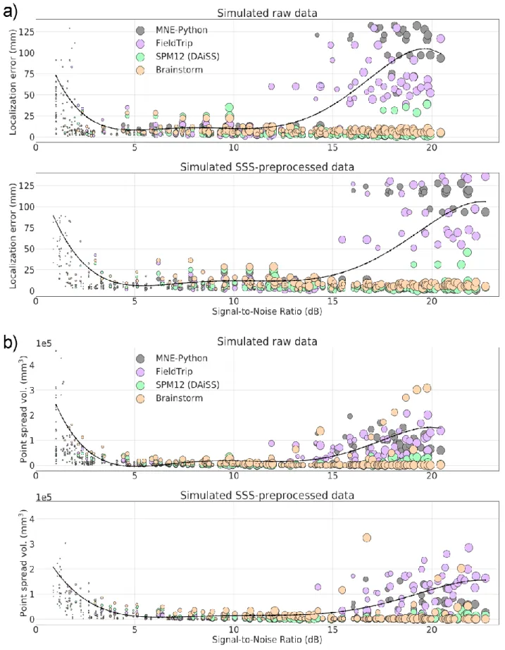
Fig. 5a shows the plots between localization error and input SNR of each simulated dataset. The 414
polynomial regressions of the maximum localization errors across LCMV implementations show the 415
variation of localization errors over the range of input SNRs. The localization error goes high for all 416
toolboxes for very low SNR (< 3 dB) signals (e.g. 20-nAm or deep sources). The localization error 417
within the input SNR range 3–12 dB is stable and mostly within 15 mm, and SSS preprocessing 418
widens this SNR range of stable performance to 3–15 dB. Unexpectedly, we also found high 419
localization error at high SNR (> 15 dB) for the toolboxes other than SPM12 (DAiSS). Fig. 5b plots 420
PSV values against input SNR for raw and SSS-preprocessed simulated data. The polynomial 421
regression plots fit a nonlinear relationship between the input SNR and the corresponding maximal 422
PSVs across the four LCMV implementations. The regression plots in Fig. 5b agree with the 423
corresponding plots in Fig. 5a, i.e., lower PSV values (higher spatial resolution) for the SNR range 424
with smaller localization errors and vice-versa, for all toolboxes. The low SNR signals (usually, weak 425
or deep sources) shows high PSV values in Fig. 5b which also indicates improved spatial resolution 426
after SSS preprocessing. Fig. 5a–b shows that none of the four toolboxes provides accurate 427
localization for all SNR values and that the spatial resolution of LCMV is dependent on input SNR. 428
SPM12 (DAiSS) shows lower localization errors and PSV values at very high SNR too. 429
Insert Fig. 5 about here
430431
3.2. Static and moving phantom MEG data
432
In the case of phantom data, the background noise is very low and there is a single source 433
underneath a measurement. Also, the phantom analysis uses a homogeneous sphere model that 434
does not introduce any forward model inaccuracy, except the possible co-registration error. All four 435
toolboxes show high localization accuracy and high resolution for phantom data, if the input SNR is 436
not very low. Corresponding results for the static phantom data are presented in Fig. 6a–b. Fig. 6a 437
indicates the localization error clear dependency on SNR. The nonlinear regression plots fitted over 438
maximum localization errors indicate high localization errors at very low SNR raw data sets. The 439
16
high error is because of some unfiltered artifacts in raw data which was removed by SSS. After SSS, 440
the beamformer shows localization error under ~5 mm for all the datasets. Fig. 6b shows the 441
beamforming resolution in terms of PSV. The regression plots fitted over maximum PSV values show 442
a high spatial resolution for the data with SNR > 5 dB. 443
444
Insert Fig. 6 about here 445
446
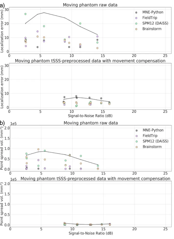
In the cases of moving phantom, Fig. 7a shows high localization errors with unprocessed raw data 447
because of disturbances caused by the movement. The dipole excitation amplitude was 200 nAm, 448
which is enough to provide a good SNR. The most superficial dipoles (Dipoles 5 and 9 in Fig. 3c) 449
possess higher SNR but also higher localization error since they get more significant angular 450
displacement during movement. Because of differences in implementations and preprocessing 451
parameters listed in Section 2.4, apparent differences among the estimated localization error can be 452
seen. Overall, MNE-Python shows the lowest while SPM12 (DAiSS) shows the highest localization 453
error with the phantom data with movement artifact. After applying for spatiotemporal tSSS and 454
movement compensation, the improved SNR provided significantly better localization accuracies. 455
Fig. 7b shows the PSV for moving phantom data for raw and processed data. The regression plots 456
indicate improvement in SNR and spatial resolution after tSSS with movement compensation. 457
458
Insert Fig. 7 about here 459
460
3.3. Human subject MEG data
461
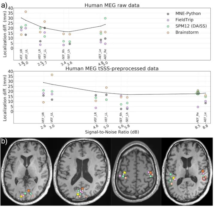
Since the correct source locations for the human evoked field datasets are unknown, we plotted the 462
localization difference across the four LCMV implementations for each data. These localization 463
differences were the Cartesian distance between an LCMV-estimated location and the 464
corresponding reference dipole location as explained in Section 2.1.4. Fig. 8a shows the plots for 465
the localization differences against the input SNRs computed using Eq (9) for four visual, two 466
auditory and two somatosensory evoked-field datasets. The localization differences for both 467
unprocessed raw and SSS preprocessed data are mostly under 20 mm in each toolbox. The higher 468
differences compared to the phantom and simulated dataset could be because of two reasons. First, 469
the recording might have been comprised by some head movement, which could not be corrected 470
because of the lack of continuous HPI. Second, the reference dipole location may not represent the 471
very same source as estimated by the LCMV beamformer. In contrast to dipole fitting, beamforming 472
utilizes data from the full covariance window, so some difference between the estimated localizations 473
17
is to be expected. For all SSS-preprocessed evoked field datasets, Fig. 8b shows the estimated 474
locations across the four LCMV implementation and the corresponding reference dipole locations. 475
For simplifying the visualization, all estimated locations in a stimulus category are projected onto a 476
single axial slice. All localizations seem to be in the correct anatomical regions, except the estimated 477
location from right-ear auditory responses by MNE-Python after SSS-preprocessing (Fig. 8b; red 478
circle). After de-selecting the channels close to the right auditory cortex, the MNE-Python-estimated 479
source location was correctly in the left cortex (Fig. 8b; green circle). The regression plots fitted over 480
the maxima of the localization differences across the LCMV implementations show the improvement 481
in input SNR and also localization improvement in some cases. Fig. 9 in Supplementary material 482
shows the PSV values as a function of the input SNR for the evoked-field datasets, demonstrating 483
the spatial resolution of beamforming. 484
485
Insert Fig. 8 about here 486
487 488
18
4. Discussion
489
The localization accuracy and beamformer resolution as a function of the input SNR were 490
investigated and compared across the LCMV implementations in the four tested toolboxes. In the 491
absence of background noise, the phantom data showed high localization accuracy and high spatial 492
resolution if the input SNR >~5 dB. All implementations also showed high localization accuracy for 493
data recording from a moving phantom after compensating the movement and applying tSSS. For 494
the simulated datasets with realistic background noise, the regression curve fitted over the maximum 495
localization error across the LCMV implementations indicates that the reliability of localization 496
accuracy in these implementations depends on the SNR of input data and these implementations 497
localize a single source reliably within the SNR range of ~3–15 dB. Small differences among the 498
estimated source locations across the implementations even in this SNR range are caused by 499
differing processing steps in defining the head model, spatial filter and performing the beamformer 500
scan. For the human subject evoked-field MEG data, all implementations localize sources within 501
about 20 mm. 502
Our results indicate that with the default parameter settings, none of the four implementations works 503
universally reliable for all datasets and input SNR values. In the case of low SNR (typically less than 504
3 dB), the lower contrast between data and noise covariance may cause the beamformer scan to 505
provide a flat peak in the output and so the localization error goes high. Unexpectedly, we found high 506
localization error for high SNR signal and significant differences between the toolboxes. The 507
regression curves fitted over averaged maximum PSV across all toolboxes showed higher values 508
for low- and high-SNR simulated data. As expected, reliable localization provides higher spatial 509
resolution across the implementations and vice-versa (Fig. 5 and 6). The lower spatial resolution 510
(higher PSV) for the signal with low SNR also agrees with previous studies (Lin et al., 2008; 511
Hillebrand and Barnes, 2003). We further discuss here the significant steps of the beamformer 512
pipelines, which affect the localization accuracy and introduce discrepancies among the 513
implementations. 514
4.1 Preprocessing with SSS 515
Due to the spatial-filter nature of the beamformer, it can reject external interference and therefore 516
SSS-based pre-processing may have little effect on the results. Thus, although the SNR increases 517
as a result of applying SSS, the localization accuracy does not necessarily improve, which is evident 518
in the localization of the evoked responses (Fig. 8). 519
However, undetected artifacts, such as a large-amplitude signal jump in a single sensor, may in SSS 520
processing spread to neighboring channels and subsequently reduce data quality. Therefore, 521
channels with distinct artifacts should be noted and marked as bad prior to beamforming of 522
unprocessed data or before applying SSS operations. In addition, trials with large artifacts should be 523
removed based on an amplitude thresholding or by other means. Furthermore, SSS processing of 524
19
extremely weak signals (SNR < ~2 dB) may not improve the SNR for producing smaller localization 525
errors and PSV values. Hence the data quality should be carefully inspected before and after 526
applying preprocessing methods such as SSS, and channels or trials with low-quality data (or lower 527
contrast) should be omitted from the covariance estimation. 528
4.2. Effect of filtering and artifact-removal methods 529
All four toolboxes we tested employ either a MATLAB or Python implementation of the same MNE 530
routines (Gramfort et al. 2014) for reading FIFF data files and thus have internally the exact same 531
data at the very first stage (see Suppl. Fig. 6). The data import either keeps the data in SI-units (T 532
for magnetometers and T/m for gradiometers) or rescales the data (fT and fT/mm) before further 533
processing. The actual pre-processing steps in the pipeline may contribute to differences in the 534
results. The filtering step is performed to remove frequency components of no interest, such as slow 535
drifts, from the data. By default, FieldTrip and SPM use an IIR (Butterworth) filter, and MNE-Python 536
uses FIR filters. The power spectra of these filters’ output signals show notable differences and the 537
output data from these two filters are not identical. Significant variations can be found between MNE-538
Python-filtered and FieldTrip/SPM-filtered data. Although SPM and FieldTrip use the same filter 539
implementation, the filtering results are not identical because of numeric differences caused by 540
different channel scaling (Suppl. Fig 6). These differences affect the estimated covariance matrices, 541
which are a crucial ingredient for the spatial-filter computation and finally may contribute to 542
differences in beamforming results. 543
4.3. Effect of SNR on localization accuracy 544
We reduced the impact of the unknown source depth and strength to a well-defined metrics in terms 545
of the SNR. We observed that the localization accuracy is poor for very low SNR values, i.e. below 546
3 dB. The weaker, as well as the deeper sources, project less power on to the sensor array and thus 547
show lower SNR; see Eq (9). On the other hand, the LCMV beamformer may also fail to localize 548
accurately sources that produce very high SNR values, likely because the data covariance matrix is 549
over-fitted, or the scanning grid is too sparse with respect to the point spread of the beamformer 550
output. In this case the output is too focal and a small error in forward solution, introduced for 551
example by inaccurate coregistration, may lead to missing the true focal source and obtaining nearly 552
equal power estimates at many source locations, increasing the chance of mislocalization. Usually, 553
such high levels of SNR do not occur in typical human MEG experiments, however, the strength of 554
equivalent current dipoles (ECD) for interictal epileptiform discharges (IIEDs) typically ranges 555
between 50 and 500 nAm (Bagic et al., 2011a). 556
All four beamformer pipelines provided very similar results when the SNR is in the “suitable range” 557
of about ~3–15 dB. Unsatisfactory performance is typically due to the data; either the SNR is 558
extremely low, or there are some uncorrected artifacts in the data. The results of the phantom data 559
20
showed that all toolboxes provide equally good results if there are no uncorrected large artifacts in 560
the data and if the SNR is not extremely small or large. 561
4.4. Effect of the head model 562
Forward modelling requires MEG–MRI co-registration, segmentation of the head MRI and leadfield 563
computation for the source space. The four beamformer implementations use different approaches, 564
or similar approaches but with different parameters, which yields slightly different forward models. 565
From Eqs (2–7), it is evident that beamformers are quite sensitive to the forward model. Hillebrand 566
and Barnes (2003) showed that the spatial resolution and the localization accuracy of a beamformer 567
improve with accuracy of the forward model. Dalal and colleagues (2014) reported that co-568
registration errors contribute greatly to EEG localization inaccuracy, likely due to their ultimate impact 569
on head-model quality. Chella and colleagues (2019) presented the dependency of beamformer-570
based functional connectivity estimates on MEG-MRI co-registration accuracy. 571
The increasing inter-toolbox localization differences towards very low and very high input SNR is 572
also subject to the differences between the head models. Fig. 4 shows the three overlapped head 573
models prepared from the same MRI where a slight misalignment among head models can be easily 574
seen. This misalignment also affects source space. These differences in head models and thus in 575
forward solutions will contribute to differences in beamforming results across the toolboxes. 576
4.5.
Covariance matrix 577The data covariance matrix is a key component of the adaptive spatial filter in LCMV beamforming, 578
and any error in covariance estimation can cause an error in source estimation. We used 5% of the 579
mean variance of all sensors to regularize data covariance for making its inversion stable in FieldTrip, 580
SPM12 and MNE-Python. Brainstorm uses a slightly different approach and applies regularization 581
with 5% of mean variance of gradiometer and magnetometer channel sets separately and eliminate 582
cross-sensor-type entries from the covariance matrices. As SSS preprocessing reduces the rank of 583
the data, usually retaining at most 75 non-zero eigenvalues, the trace of the covariance matrix 584
decreases strongly. At very high SNRs (> 15 dB), overfitting of the covariance matrix becomes more 585
prominent; the condition number (ratio of the largest and the smallest eigenvalues) of the covariance 586
matrix becomes very high even after the default regularization, which can deteriorate the quality of 587
source estimates unless the covariance is appropriately regularized. Therefore, the seemingly same 588
5% regularization can have very different effects before and after SSS; see Suppl. Fig. 7. Thus, the 589
commonly used way of specifying the regularization level might not be appropriate to produce a good 590
and stable covariance model at high SNR, and this could be one of the explanations for the 591
anecdotally reported detrimental effects of SSS on beamforming results. 592
21
5. Conclusion
593
We conclude that with the current versions of LCMV beamformer implementations in the four open-594
source toolboxes — FieldTrip, SPM12(DAiSS), Brainstorm, and MNE-Python — the localization 595
accuracy is acceptable (within ~10 mm for a true point source) for most purposes when the input 596
SNR is 3–15 dB. Lower or higher SNR may compromise the localization accuracy and spatial 597
resolution. To extend this useable range, a properly defined scaling strategy such as pre-whitening 598
should be implemented across the toolboxes. The default regularization is often inadequate and may 599
yield suboptimal results. Therefore, a data-driven approach for regularization should be adopted to 600
alleviate problems with low- and high-SNR cases. Our further work will be focusing on optimizing 601
regularization using a more data-driven approach. 602
603
Acknowledgment
604
This study has been supported by the European Union H2020 MSCA-ITN-2014-ETN program, 605
Advancing brain research in Children’s developmental neurocognitive disorders project (ChildBrain 606
#641652). SSD and BUW have been supported by an ERC Starting Grant (#640448). 607
608
References
609
Bagic, A. I., Knowlton, R. C., Rose, D. F., Ebersole, J. S., & ACMEGS Clinical Practice Guideline 610
(CPG) Committee. (2011a). American clinical magnetoencephalography society clinical practice 611
guideline 1: recording and analysis of spontaneous cerebral activity. J Clin Neurophysiol. 28(4): 348– 612
354. http://dx.doi.org/10.1097/WNP.0b013e3182272fed 613
Bagic, A. I., Knowlton, R. C., Rose, D. F., Ebersole, J. S., & ACMEGS Clinical Practice Guideline 614
(CPG) Committee. (2011b). American Clinical Magnetoencephalography Society Clinical Practice 615
Guideline 3: MEG–EEG Reporting. J Clin Neurophysiol. 28(4): 362–365. 616
http://dx.doi.org/10.1097/WNO.0b013e3181cde4ad 617
Barca, L., Cornelissen, P., Simpson, M., Urooj, U., Woods, W., & Ellis, A. W. (2011). The neural 618
basis of the right visual field advantage in reading: an MEG analysis using virtual electrodes. Brain 619
Lang 118(3): 53–71. http://dx.doi.org/10.1016/j.bandl.2010.09.003 620
Burgess, R. C., Funke, M. E., Bowyer, S. M., Lewine, J. D., Kirsch, H. E., Bagić, A. I., & ACMEGS 621
Clinical Practice Guideline (CPG) Committee (2011). American Clinical Magnetoencephalography 622
Society Clinical Practice Guideline 2: Presurgical functional brain mapping using magnetic evoked 623
fields. J Clin Neurophysiol. 28(4): 355–361. http://dx.doi.org/10.1097/WNP.0b013e3182272ffe 624
22
Chella, F., Marzetti, L., Stenroos, M., Parkkonen, L., Ilmoniemi, R. J., Romani, G. L., & Pizzella, V. 625
(2019). The impact of improved MEG–MRI co-registration on MEG connectivity analysis. 626
NeuroImage, 197: 354-367. https://doi.org/10.1016/j.neuroimage.2019.04.061 627
Dalal, S. S., Rampp, S., Willomitzer, F., & Ettl, S. (2014). Consequences of EEG electrode position 628
error on ultimate beamformer source reconstruction performance. Front Neurosci. 8: 42. 629
http://dx.doi.org/10.3389/fnins.2014.00042 630
Dale, A. M., Fischl, B., & Sereno, M. I. (1999). Cortical surface-based analysis I: Segmentation and 631
surface reconstruction. Neuroimage 9(2): 179-194. https://doi.org/10.1006/nimg.1998.0395 632
Dale, A. M., Liu, A. K., Fischl, B. R., Buckner, R. L., Belliveau, J. W., Lewine, J. D., & Halgren, E. 633
(2000). Dynamic statistical parametric mapping: combining fMRI and MEG for high-resolution 634
imaging of cortical activity. Neuron 26(1): 55–67. http://dx.doi.org/10.1016/S0896-6273(00)81138-1 635
Elekta Neuromag® TRIUX User’s Manual, (Megin Oy, 2018)
636
Engemann, D. A., & Gramfort, A. (2015). Automated model selection in covariance estimation and
637
spatial whitening of MEG and EEG signals. NeuroImage 108: 328–342.
638
http://dx.doi.org/10.1016/j.neuroimage.2014.12.040
639
Fischl, B. (2012). FreeSurfer. Neuroimage 62(2): 774–781. 640
https://doi.org/10.1016/j.neuroimage.2012.01.021 641
Fischl, B., Sereno, M. I. & Dale, A. M. (1999). Cortical surface-based analysis II: Inflation, flattening, 642
and a surface-based coordinate system. NeuroImage 9(2): 195–207.
643
https://doi.org/10.1006/nimg.1998.0396 644
Gramfort, A., Luessi, M., Larson, E., Engemann, D. A., Strohmeier, D., Brodbeck, C., ... & 645
Hämäläinen, M. (2013a). MEG and EEG data analysis with MNE-Python. Front Neurosci. 7: 267. 646
http://dx.doi.org/10.3389/fnins.2013.00267 647
Gramfort, A., Strohmeier, D., Haueisen, J., Hämäläinen, M. S., & Kowalski, M. (2013b). Time-648
frequency mixed-norm estimates: Sparse M/EEG imaging with non-stationary source activations. 649
NeuroImage 70: 410–422. http://dx.doi.org/10.1016/j.neuroimage.2012.12.051 650
Gramfort, A., Luessi, M., Larson, E., Engemann, D. A., Strohmeier, D., Brodbeck, C., ... & 651
Hämäläinen, M. S. (2014). MNE software for processing MEG and EEG data. Neuroimage 86: 446– 652
460. http://dx.doi.org/10.1016/j.neuroimage.2013.10.027 653
Gross, J., Kujala, J., Hämäläinen, M., Timmermann, L., Schnitzler, A., & Salmelin, R. (2001). 654
Dynamic imaging of coherent sources: studying neural interactions in the human brain. Proc Natl 655
Acad Sci USA 98(2): 694-699. http://dx.doi.org/10.1073/pnas.98.2.694 656
23
Hall, M. B., Nissen, I. A., van Straaten, E. C., Furlong, P. L., Witton, C., Foley, E., ... & Hillebrand, A. 657
(2018). An evaluation of kurtosis beamforming in magnetoencephalography to localize the 658
epileptogenic zone in drug-resistant epilepsy patients. Clin Neurophysiol. 129(6): 1221–1229. 659
http://dx.doi.org/10.1016/j.clinph.2017.12.040 660
Hämäläinen, M., Hari, R., Lounasmaa, O. V., Knuutila, J., & Ilmoniemi, R. J. (1993). 661
Magnetoencephalography-theory, instrumentation, and applications to noninvasive studies of the 662
working human brain. Rev Mod Phys 65: 413–497. https://doi.org/10.1103/RevModPhys.65.413 663
Hämäläinen, M. S., & Ilmoniemi, R. J. (1994). Interpreting magnetic fields of the brain: minimum 664
norm estimates. Med Biol Eng Compt. 32(1): 35–42. https://doi.org/10.1007/BF02512476 665
Hämäläinen, M. S., & Sarvas, J. (1989). Realistic conductivity geometry model of the human head 666
for interpretation of neuromagnetic data. IEEE Trans Biomed Eng. 36(2): 165–171. 667
https://doi.org/10.1109/10.16463 668
Hillebrand, A., & Barnes, G. R. (2003). The use of anatomical constraints with MEG beamformers.
669
Neuroimage 20(4): 2302–2313. http://dx.doi.org/10.1016/j.neuroimage.2003.07.031
670
Hillebrand, A., & Barnes, G. R. (2005). Beamformer analysis of MEG data. Int Rev Neurobiol 68: 671
149–171. http://dx.doi.org/10.1016/S0074-7742(05)68006-3 672
Huang, M. X., Mosher, J. C., & Leahy, R. M. (1999). A sensor-weighted overlapping-sphere head 673
model and exhaustive head model comparison for MEG. Phys Med Biol. 44(2): 423-440. 674
http://dx.doi.org/10.1088/0031-9155/44/2/010
675
Ilmoniemi, R. J., Hämäläinen, M. S., & Knuutila, J. (1985). The forward and inverse problems in the 676
spherical model, in: Weinberg, H., Stroink, G. & Katila, T. (Eds.), Biomagnetism: Applications and 677
Theory. Pergamon Press, New York, 278–282 678
Ilmoniemi, R. J., & Sarvas, J. (2019). Brain Signals: Physics and Mathematics of MEG and EEG.
679
MIT Press.
680
Ishii, R., Canuet, L., Ishihara, T., Aoki, Y., Ikeda, S., Hata, M., ... & Iwase, M. (2014). Frontal midline 681
theta rhythm and gamma power changes during focused attention on mental calculation: an MEG 682
beamformer analysis. Front Hum Neurosci. 8: 406. http://dx.doi.org/10.3389/fnhum.2014.00406 683
Lin, F. H., Witzel, T., Zeffiro, T. A., & Belliveau, J. W. (2008). Linear constraint minimum variance
684
beamformer functional magnetic resonance inverse imaging. Neuroimage 43(2): 297–311.
685
http://dx.doi.org/10.1016/j.neuroimage.2008.06.038 686
Litvak, V., Mattout, J., Kiebel, S., Phillips, C., Henson, R., Kilner, J., ... & Penny, W. (2011). EEG and 687
MEG data analysis in SPM8. Comput Intell Neurosci. 2011. http://dx.doi.org/10.1155/2011/852961 688
24
Mattout, J., Henson, R. N., & Friston, K. J. (2007). Canonical source reconstruction for MEG. Comput 689
Intell Neurosci. 2007. http://dx.doi.org/10.1155/2007/67613 690
Mosher, J. C., Lewis, P. S., & Leahy, R. M. (1992). Multiple dipole modeling and localization from 691
spatio-temporal MEG data. IEEE Trans Biomed Eng. 39(6): 541–557. 692
http://dx.doi.org/10.1109/10.141192 693
Nenonen J, Nurminen J, Kicic D, Bikmullina R, Lioumis P, Jousmäki V, Taulu S, Parkkonen L, 694
Putaala M, Kähkönen S (2012). Validation of head movement correction and spatiotemporal signal 695
space separation in magnetoencephalography. Clin Neurophysiol. 123(11): 2180–2191. 696
http://dx.doi.org/10.1016/j.clinph.2012.03.080 697
Nolte, G. (2003). The magnetic lead field theorem in the quasi-static approximation and its use for 698
magnetoencephalography forward calculation in realistic volume conductors. Phys Med Biol. 48(22): 699
3637. http://dx.doi.org/10.1088/0031-9155/48/22/002 700
Oostenveld, R., Fries, P., Maris, E., & Schoffelen, J. M. (2011). FieldTrip: open source software for 701
advanced analysis of MEG, EEG, and invasive electrophysiological data. Comput Intell Neurosci. 702
2011. http://dx.doi.org/10.1155/2011/156869 703
Pascual-Marqui, R. D., Michel, C. M., & Lehmann, D. (1994). Low resolution electromagnetic 704
tomography: a new method for localizing electrical activity in the brain. Int J Psychophysiol. 18(1): 705
49-65. https://doi.org/10.1016/0167-8760(84)90014-X 706
Robinson S.E., Vrba, J. (1998). Functional neuroimaging by synthetic aperture magnetometry 707
(SAM), in: Yoshimoto, T., Kotani, M., Kuriki, S., Karibe, H. & Nakasato, N. (Eds.), Recent Advances 708
in Biomagnetism. Tohoku University Press, Japan, 302–305. 709
Salmelin, R. (2010). Multi-dipole modeling in MEG, in: Hansen, P., Kringelbach, M. & Salmelin, R. 710
(Eds.), MEG: an introduction to methods. Oxford university press, 124–155. 711
http://dx.doi.org/10.1093/acprof:oso/9780195307238.003.0006 712
Sekihara, K., & Scholz, B. (1996). Generalized Wiener estimation of three-dimensional current 713
distribution from biomagnetic measurements. IEEE Trans Biomed Eng. 43(3): 281-291. 714
http://dx.doi.org/10.1109/10.486285 715
Sekihara, K., Hild, K. E., & Nagarajan, S. S. (2006). A novel adaptive beamformer for MEG source 716
reconstruction effective when large background brain activities exist. IEEE Trans Biomed Eng. 53(9), 717
1755–1764. http://dx.doi.org/10.1109/TBME.2006.878119 718
Sekihara, K., & Nagarajan, S., S. (2008). Adaptive spatial filters for electromagnetic brain imaging.
719
Springer Science & Business Media.https://doi.org/10.1007/978-3-540-79370-0 720


![[PDF] Introduction au cours UML Use Case et méthodes | Cours uml](data:image/gif;base64,R0lGODlhAQABAIAAAP///wAAACH5BAEAAAAALAAAAAABAAEAAAICRAEAOw==)