A modified Generalized Least Squares method for large scale nuclear data evaluation

(1)

HAL Id: hal-01465923

https://hal.archives-ouvertes.fr/hal-01465923

Submitted on 13 Feb 2017

HAL is a multi-disciplinary open access

archive for the deposit and dissemination of

sci-entific research documents, whether they are

pub-lished or not. The documents may come from

teaching and research institutions in France or

abroad, or from public or private research centers.

L’archive ouverte pluridisciplinaire HAL, est

destinée au dépôt et à la diffusion de documents

scientifiques de niveau recherche, publiés ou non,

émanant des établissements d’enseignement et de

recherche français ou étrangers, des laboratoires

publics ou privés.

A modified Generalized Least Squares method for large

scale nuclear data evaluation

Georg Schnabel, Helmut Leeb

To cite this version:

Georg Schnabel, Helmut Leeb. A modified Generalized Least Squares method for large scale

nu-clear data evaluation.

Nuclear Instruments and Methods in Physics Research Section A:

Ac-celerators, Spectrometers, Detectors and Associated Equipment, Elsevier, 2017, 841, pp.87 - 96.

�10.1016/j.nima.2016.10.006�. �hal-01465923�

(2)

Contents lists available atScienceDirect

Nuclear Instruments and Methods in Physics Research A

journal homepage:www.elsevier.com/locate/nima

A modi

ﬁed Generalized Least Squares method for large scale nuclear data

evaluation

Georg Schnabel

a,b,⁎

, Helmut Leeb

b

a_{Irfu, CEA, Université Paris-Saclay, 91191 Gif-sur-Yvette, France} b_{Atominstitut, TU Wien, Vienna, Austria}

A R T I C L E I N F O

Keywords:

Nuclear data evaluation Generalized Least Squares Bayesian statistics

A B S T R A C T

Nuclear data evaluation aims to provide estimates and uncertainties in the form of covariance matrices of cross sections and related quantities. Many practitioners use the Generalized Least Squares (GLS) formulas to combine experimental data and results of model calculations in order to determine reliable estimates and covariance matrices. A prerequisite to apply the GLS formulas is the construction of a prior covariance matrix for the observables from a set of model calculations. Modern nuclear model codes are able to provide predictions for a large number of observables. However, the inclusion of all observables may lead to a prior covariance matrix of intractable size. Therefore, we introduce mathematically equivalent versions of the GLS formulas to avoid the construction of the prior covariance matrix. Experimental data can be incrementally incorporated into the evaluation process, hence there is no upper limit on their amount. We demonstrate the modiﬁed GLS method in a tentative evaluation involving about three million observables using the code TALYS. The revised scheme is well suited as building block of a database application providing evaluated nuclear data. Updating with new experimental data is feasible and users can query estimates and correlations of arbitrary subsets of the observables stored in the database.

1. Introduction

The increasing performance of computers and the availability of computer clusters enable nowadays simulations of complex nuclear systems such as reactors. These simulations guide design choices regarding eﬃciency and safety. An important prerequisite for such simulations are reliable estimates of reaction cross sections and emission spectra. There is also an increasing demand for uncertainty information in the form of covariance matrices. Usually, perturbation theory is used to propagate these uncertainties through simulations in order to obtain the corresponding uncertainties of the integral ob-servables (e.g.[1]). An alternative to perturbation theory is the total Monte Carlo method[2]. The latter is able to deal with non-Gaussian distributions but is computationally more demanding[3]. Therefore, perturbation theory using covariance matrices remains a viable option for uncertainty propagation.

Estimates and covariance matrices are generated with the help of an evaluation method. An evaluation method is a statistical procedure which combines results of model calculations and experimental data to obtain an improved set of estimates and covariance matrices for the observables. Several evaluation methods were proposed (e.g.[4–13]) which diﬀer in their details but commonly employ the framework of

Bayesian statistics. For an overview of the diﬀerent methods see e.g. [14]and[15, pp. 61–74].

The basic formulas used by most of these methods are often referred to as Generalized Least Squares (GLS) formulas. There are two approaches to include information of a nuclear model into the GLS formulas. In the linearization approach, one linearizes the model and assumes a multivariate normal distribution for the model parameters (e.g.[5,7]). In the sampling approach, one creates a sample of model calculations with varied model parameters and constructs a multi-variate normal distribution for the predicted observables (e.g.[9,11]). The linearization approach requires only a small number of model parameters to be updated. The advantage of the sampling approach is that it allows evaluations to better resemble experimental data because theﬁnal evaluation does not necessarily need to correspond to a model prediction with a speciﬁc choice of model parameters[15, p. 37–41]. However, a disadvantage of the sampling approach is its restriction on the number of observables which can be taken into account.

Nuclear model codes such as TALYS[16,17]are able to predict a number of observables in the order of millions if one considers a broad range of incident energies (e.g. between 1 and 200 MeV). Updating such a number of observables and the associated covariance matrix is troublesome using the sampling approach in combination with the

http://dx.doi.org/10.1016/j.nima.2016.10.006

Received 16 June 2016; Received in revised form 19 September 2016; Accepted 1 October 2016 ⁎_{Corresponding author at: CEA/Saclay, DRF/Irfu/SPhN, 91191 Gif-sur-Yvette Cedex, France}

Nuclear Instruments and Methods in Physics Research A 841 (2017) 87–96

(3)

standard GLS formulas.

The main obstacle for the large scale application of the GLS formulas is the prior covariance matrix for the observables. As an example, the GANDR code suite[18] developed at the International Atomic Energy Agency[19]allows the consistent evaluation of 91 000 observables on a personal computer, which involves a 91 000×91 000 covariance matrix taking about 30 gigabytes of storage space. If the number of observables were increased to millions, the covariance matrix would inﬂate to a size in the order of 10 terabytes. Consequently, the computation time would surpass an acceptable level. In this paper, we present a revised computation scheme to evaluate the GLS formulas which avoids the explicit construction of the prior covariance matrix. We exploit the fact that the L×Lcovariance matrix for L observables is constructed from a much smaller number N of model calculations (e.g.L = 106_{and N = 10}3_{). Concerns may be raised}

that estimating a covariance matrix of larger dimension than the number of model calculations is problematic from a statistical point of view. However, model predictions are determined by a limited number of parameters, hence the intrinsic dimension of the covariance matrix is much lower than its nominal dimension. The number of model calculations must be only suﬃciently larger than the intrinsic dimension to justify the application of the GLS formulas.

In order to represent an updated state of knowledge, neither updated estimates of observables nor corresponding covariance ma-trices have to be stored. It suﬃces to keep (1) a vector→w1containing a

weight for each of the N model calculations, (2) a N×N covariance matrix W1referring to model calculations instead of observables, and

(3) the results of model calculations.

Experimental data can be included in several stages, which is a signiﬁcant extension to the work presented in[20]. The time need to update the information of millions of observables based on experi-mental data is in the order of seconds on a modern personal computer. Estimates of observables and relevant pieces of the full evaluated covariance matrix can be eﬃciently reconstructed from→w1, W1and the

model calculation results.

These features make the revised GLS scheme well suited to be implemented as a database application. Estimates, uncertainties and correlations of arbitrary subsets of observables can be computed on demand. Due to the large size of a full covariance matrix for all observables, libraries such as JEFF [21] or TENDL [22] provide covariances only for the most signiﬁcant reaction channels. On the other hand, theﬂexibility of the envisaged database application would give the user the freedom to retrieve any covariance matrix which is important for his application.

Finally, we note that the idea to avoid the construction of a possibly large matrix and instead to work with the vectors from which it would be constructed has already been successfully applied in otherﬁelds and contexts, see e.g. the Ensemble Kalman Filter[23,24]and the L-BFGS method for optimization[25,26].

The structure of this paper is as follows. Section 2 provides a concise sketch of the GLS method and elaborates on the required modiﬁcations to enable the evaluation of a large number of observa-bles. Section 3 compares the time and storage requirement of the standard approach and the modiﬁed approach. Section 4 contains details about the application of the revised GLS method in an evaluation of neutron-induced reactions on 181Ta with 854 experi-mental data points and about three million observables predicted by the nuclear models code TALYS. Section 5 underlines important aspects of the revised evaluation scheme. Section 6provides conclu-sions and an outlook.

2. Method 2.1. Basic method

We give a brief sketch of the GLS method, which will serve as the

basis to discuss the modiﬁcations for a large number of observables. A derivation of the GLS formulas is given inAppendix A.

The purpose of the GLS method is to infer best estimates of observables and an associated covariance matrix by taking into account both the results of model calculations and experimental data. In the GLS method, both experimental uncertainties and the variations of model predictions due to variations of parameters are described by multivariate normal distributions.

The GLS method takes place in three steps: First, the results of model calculations are used to construct the so-called prior, deﬁned by a prior mean vector and a prior covariance matrix. Second, one assembles the measured values of experiments into a measurement vector and constructs an associated covariance matrix based on the knowledge about statistical and systematic measurement errors. And third, the quantities of theﬁrst and second steps are combined using the GLS formulas to obtain the posterior, which comprises a posterior mean vector and a posterior covariance matrix. Following, we discuss each step in more detail and provide the mathematical formulas.

Construction of the prior. Information from model calculations has to be represented by a vector of best estimates σ→0and an associated

covariance matrix A0. In order to determine these two quantities, one

performs a certain number N of model calculations with diﬀerent model parameter sets p{→i i}=1 ..N. For example, using TALYS the vectors

p →

i contain the parameters of the optical model in the global parame-trization of Koning–Delaroche [27]. The values of the parameter vectors are usually drawn from a uniform or a multivariate normal distribution. Diﬀerent procedures have been suggested to determine sensible ranges (in the case of a uniform distribution) or a center vector and a covariance matrix (in the case of a multivariate normal distribution) for the parameter vector. These procedures either make use of constraints stemming from physics considerations [11] or specify the parameter ranges in such a way that the associated predictions cover the majority of available experimental data[28].

Once the model prediction vector x→i is available for each model parameter vector→p_i in the set p{→i i}=1 ..N, the prior mean vector σ→0 and

the prior covariance matrix A0are calculated by

∑

σ N x A N x σ x σ → = 1 → _and ₌ 1 (→− → )(→− → ) . i N i i N i i T 0 =1 0 =1 0 0 (1) Another possible way to set up σ→0is to make a model calculation based

on the mean vector of the parameter distribution and to use the result as prior mean vector σ→0for the observables.

One can see from these formulas that the vector σ→0 is of the same

dimension as the model prediction vectors x→i. The position of a value in these vectors indicates to which observable this value refers. Observables predicted by a nuclear model are typically cross sections, angle-diﬀerential cross sections and spectra. However, any continuous observable predicted by a model may be used.

Experimental data. The knowledge from experimental data has to be cast into a measurement vector σ→exp and an associated experiment

covariance matrix B. The measurement vector contains the values obtained in the experiments. Of course, one has to keep track to which observables these values relate. The level of trust in the measured values is used to set up a covariance matrix B. The squared statistical uncertainties due to a limited number of detected events have to be placed in the diagonal of the covariance matrix. Systematic errors, which tie together uncertainties of different values, lead to contribu-tions to both diagonal and off-diagonal elements. For example, an uncertainty about the proper calibration of the employed detector translates to a systematic uncertainty of all cross sections of different atomic nuclei measured with the detector. More information about the construction of covariance matrices can be found in[29].

Performing the update. The information from model calculations represented by a prior center vector σ→0and a prior covariance matrix

A0provides one source of information; the information from

(4)

covariance matrix B another one. The application of the Bayesian update formulas allows us to combine these quantities to obtain the posterior center vector→σ1and the posterior covariance matrix A1. If new

measurement data are available, one can use the obtained posterior as the new prior. Hence we will use the notation→σi andAi to denote the prior of the current iteration. The Bayesian update formula to calculate the posterior mean vector σ→i+1 of the current iteration reads (see Appendix)

σ σ A S SA S B σ Sσ

→ _{= → +} ₍ ₊ _{) (→} _{− →).}

i+1 i i T i T −1 exp i (2)

The observables in→σi are usually deﬁned on a diﬀerent energy/angle grid than those in σ→exp. The sensitivity matrix S maps the observables

from the model grid associated with→σito the grid associated with σ→exp.

Depending on the choice of S, diﬀerent mapping schemes such as linear or spline interpolation are possible. In the opinion of the authors, linear interpolation has to be preferred over other interpolation schemes because it leads to very sparse matrices S, which is compu-tationally beneﬁcial. The reduced smoothness compared to e.g. splines can be compensated by using more grid points.

The posterior covariance matrix Ai+1with a reduced uncertainty is given by (see Appendix)

Ai+1=Ai−A S SA Si T( i T+B)−1SAi. (3) These update formulas are convenient tools in nuclear data evaluation due to their simplicity. The numerically most complex operation is the inversion of an M×M matrix with M being the number of measurements and thus the dimension of σ→exp. The number

L of observables in the vector→σi is from a computational perspective rather uncritical, because the corresponding L×L covariance matrix Aiis only involved in a matrix product. However, admissible computa-tion time and storage space pose practical limits on the number of observables. For instance, a TALYS calculation up to 200 MeV yields millions of predicted observables. The storage requirement of the associated covariance matrixAiwould be in the order of 10 terabytes. 2.2. Modiﬁed method

Following we describe the modiﬁed method, which enables evalua-tions with a much larger number of observables than the basic method. The methods are mathematically equivalent, which is shown inSection 2.4. Like the basic method, the input quantities of the modiﬁed method are the mean prediction vector σ→0(see Eq.(1)), the model prediction

vectors x→k and the measurement vector σ→exp with the associated

covariance matrix B. Three execution blocks can be distinguished in the modiﬁed method: constructing the prior, performing the update, and making predictions.

Constructing the prior. The quantities being updated in the modiﬁed method are a vector of weights w→i and an associated covariance matrix Wi. The dimensions are N and N×N, respectively, with N being the number of model calculations. The index i indicates that updates can be performed in several stages, where a new experimental data set is included in each stage. In the veryﬁrst update, the assignments are w→0= 0→andW0=, whereis the N×Nidentity

matrix.

Performing the update. Each update step requires the calculation of the matrix

v v v

V= (→1,→2, …,→N) (4) with vk=S(→xk− → )σ0. The matrix S maps observables from the model

grid to the energies and angles of the measurement vector σ→exp. Thus,

the ith column of V contains the prediction of a model calculation based on parameter set→pi for the experimental data set. Depending on the number of experimental data points M and the number of observables L predicted by the model code, the M×Lmatrix S can attain a signiﬁcant size. However, S is usually very sparse and this feature allows for both eﬃcient storage and computation. We elaborate

on this point in more detail inSection 2.3. The M×Nmatrix Vﬁts in typical evaluation scenarios completely into main memory. If not, the matrix products in the following equations can be performed block wise, reading the blocks of V sequentially from the hard drive.

Introducing the abbreviation ⎛ ⎝ ⎜ ⎞_⎠⎟ N Xi= 1VWVi T+B , −1 (5) we can write the update formulas as

⎛ ⎝ ⎜ ⎞_⎠⎟ w w σ σ N w WV X S V → ₌→₊ → _{− → −} 1 → _, i+1 i i T i exp 0 i (6) and N Wi+1=Wi− 1WV X VWi T i i. ₍₇₎

Noteworthy, the modiﬁed method updates the N N× matrix Wi whereas the basic method updates the L×Lmatrix Ai. Evaluations may involve N=1000 model calculations andL = 106_{observables. The}

smaller size of the matrix to be updated in the modified method is the main reason why the modified method is much faster than the basic method. We compare the differences between the methods with respect to execution time and storage requirement thoroughly inSection 3.

Making predictions. LetSP_{be the matrix that maps the observables} from the model grid to the energies and angles of interest. Using the weight vector →wi, the mean prediction vector σ→0 and the model

prediction vectors x→k, the predictions for the observables of interest are

σ σ N w S V → = → + 1 →,i P _P _P i 0 (8) whereVP_{is de}_{ﬁned as in Eq.}₍₄₎_{with S replaced by}_SP_{. The associated} covariance matrix reads

N

AiP= 1V W VP i( P T) .

(9) In contrast to the basic method, there is no need to evaluate the complete covariance matrixAi during updating. Blocks may only be computed when they are themselves of interest.

2.3. Eﬃcient mapping

Both modiﬁed update equations(6) and (7)contain the matrix V whose columns are given by vS→k=S→xk− →Sσ0. The sensitivity matrix S is

of dimension M×Lwhere M is the number of elements in σ→expand L is

the number of elements in σ→0. For instance, assuming L = 106 and

M=5000, the matrix S needs about 40 gigabytes of storage space. However, S is usually very sparse and one could exploit this sparsity to reduce the storage size. Assuming linear interpolation for cross sections, which are functions of incident energy, and bilinear inter-polation for angle-diﬀerential cross sections and spectra, which are functions of incident energy and emission energy or scattering angle, the sensitivity matrix contains not more than four non-zero elements in each row. Storing just the positions and the values of the non-zero elements, instead of M×Lnumbers only3 × 4 ×M numbers have to be stored. The sparse representation also speeds up the computation of

x

S→kand σS→0by the same factor.

Furthermore, it is possible to avoid completely the explicit deter-mination of S. The only purpose of S is to interpolate observables from the model grid to the experiment grid. The multiplication with S can therefore be replaced by directly performing the required interpolation. Because the task to compare model predictions with experimental data is quite common, scripts to interpolate results of model calcula-tions to the energies and angles of the experimental data are often available. Building on existing scripts, the modiﬁed GLS method can be quickly implemented in a high-level language like R or MatLab.

G. Schnabel, H. Leeb Nuclear Instruments and Methods in Physics Research A 841 (2017) 87–96

(5)

2.4. Derivation of the modiﬁed method

The modiﬁed method presented in Section 2.2 is the direct consequence of a reformulation which is outlined in the following. For a concise notation, we introduce the shifted prediction vectors

u x σ

→₌→_{− →}

k k 0and reiterate the abbreviation v→k=S→uk. We bundle these quantities to matrices of dimension L×Nand M×N respectively,

u u u v v v

U= (→1,→2, …,→N) and V= (→1,→2, …,→N). (10) Key idea of the modiﬁed GLS method is to avoid the explicit computation of the prior covariance matrix. Therefore, we introduce an

N×N matrix Wi and rewrite the prior covariance matrixAi of some iteration i as

∑ ∑

N u W u N Ai= 1 → → = 1UWU . j N j k N j i jk k T i T =1 = , (11) In the veryﬁrst update, the choiceW0=yields the prior covariance A0

given in Eq.(1). In later update iterations, the respective matrix Wiwill in general also contain non-diagonal elements. We use this decom-position ofAito express the inverted matrix occurring in Eqs.(2) and

(3)as ⎛ ⎝ ⎜ ⎞_⎠⎟ N Xi= (SA Si T+B)−1= 1VWVi T+B . −1 (12) Using the introduced notation, we can rewrite Eq.(2)

∑

σ σ N σ σ σ N u u σ σ UWV X S UWV X S → _{= → +} 1 (→ − →) = → + 1 →[→ (→ − →)]. i i i T i i i k N k k T i T i i +1 exp =1 exp (13) The expression in the squared bracket at the end is just a number. Therefore, the diﬀerence σ→i+1− →σi can be described as a linear combination of the shifted model prediction vectors→uk.

This feature allows us to express→σiof any iteration i in the form

∑

σ σ N u w σ NUw → = → + 1 → _{= → +} 1 →_, i k N k ik i 0 =1 0 (14) where the vectors→wihave to be determined during updating. In theﬁrst update iteration, we have w→0= 0→. Inserting Eq.(14)into Eq.(13)leads to ⎛ ⎝ ⎜ ⎞_⎠⎟ ⎧ ⎨ ⎩ ⎛ ⎝ ⎜ ⎞_⎠⎟⎫⎬ ⎭ σ σ N w N σ σ N w N w σ σ N w N w U UWV X S V U WV X S V U → _{− → =} 1 →₊ 1 → _{− → −} 1 → = 1 →+ → − → − 1 → = 1 → . i i i T i i i i T i i i +1 0 exp 0 exp 0 +1 (15) The result of this update formula can be written as the product of U and an updated vector of weights w→i+1. Therefore, it suﬃces to consider the reduced update equation

⎛ ⎝ ⎜ ⎞_⎠⎟ w w σ σ N w WV X S V → ₌→₊ → _{− → −} 1 →_, i+1 i i T i exp 0 i (16) which is exactly Eq.(6)in the outline of the modiﬁed method inSection 2.2.

We proceed with the calculation of Ai+1. Inserting Eq.(11)into the update Eq.(3)gives

N N

Ai+1= 1UWUi T− 1₂UWV X VWUi T i i T

(17) ⎛ ⎝ ⎜ ⎞_⎠⎟ N N N Ai+1= 1U Wi− 1WV X VW Ui T i i T= 1UWi+1UT. (18) Thus, we just consider the update equation

N

Wi+1=Wi− 1WV X VWi T i i, ₍₁₉₎

whose structure resembles the original update equation (3). This update equation appears as Eq. (7) in the outline of the modiﬁed method inSection 2.2. Similar to the original update equations(2) and (3), also the modiﬁed equations(16) and (19)allow the inclusion of experimental data in several stages.

Predictions of observables can be computed by taking recourse to Eq.(14). LetSP _{be the matrix to map from the model grid to the} energies and angles of interest. Multiplying Eq.(14)from the left bySP yields σ σ N w S V → = → + 1 →i P _P i 0 ₍₂₀₎ with σ→ = →i S σ P _P

i. Similarly, multiplying Eq.(18)from the left bySPand from the right by S( P T) _{and substituting i}_{( + 1) →}_i_gives

N Ai = 1V W V( ) P P i P T (21) with Ai =S A S( ) P P

i P Tcommonly known as sandwich formula.

3. Comparison of methods

Flow charts of the standard and the revised GLS scheme are shown inFig. 1. The most important diﬀerence between them is that updating and making predictions are clearly separated processes in the revised scheme. To enable updating with experimental data in several stages in the standard scheme, the full covariance matrixAihas to be updated within each stage. If the employed nuclear model predicts e.g.L = 106

diﬀerent observables, the L L× posterior covariance matrix would need about 4 terabytes of storage space. While this amount of storage space may be available on a well-equipped personal computer, the calculation of the posterior covariance matrix and writing it to disk takes considerable time. How much time will be studied in the course of this section.

In contrast to that, an update in the revised scheme consists of updating the auxiliary quantities→wiand Wiof dimension N and N×N, respectively, with N being the number of performed model calcula-tions. Typically, N is in the order of 103 _{and therefore the storage}

requirement of Wi about 400 megabytes—a remarkable reduction compared to the earlier mentioned 4 terabytes ofAi.

The auxiliary quantities→wiand Wiin combination with the vector σ→0

and the model prediction vectors x→kcompletely characterize the current state of knowledge. On their basis, predictions of observables and associated covariance matrices can be calculated whenever needed. We emphasize again the important diﬀerence to the standard scheme, in which the full set of predictions and the associated covariance matrix must be calculated during updating.

Having outlined the conceptional diﬀerences between the two schemes, we want to test their performance in practice, such as their time need. Because the time need depends on the employed computer as well as the used programming language, we feel obliged to provide these technical details. The calculations presented in the next two subsections were performed on a computer equipped with an Intel i5-3550 processor with four cores at 3.3 GHz, 32 gigabytes of main memory, and a solid-state drive. The throughput of the solid-state drive has been measured to be around 350 megabytes a second. We used the programming language R [30] to implement the matrix formulas. This language relies on the Basic Linear Algebra Subprogram routines to perform basic linear algebra operations. We employed the optimized OpenBLAS[31]implementation which makes use of all available cores in parallel. In order to work with matrices whose size exceeds available main memory, we employed the bigmem-ory[32]package. Using this package, matrices are stored inﬁles but within R they can be treated as if they would be located in the main memory.

(6)

3.1. Prior generation

Both schemes contain a prior generation phase. In the standard scheme, this phase includes the construction of the prior mean vector

σ

→

0and the associated prior covariance matrix A0. The prior generation

in the revised scheme comprises the construction of σ→0, the

determina-tion of the model predicdetermina-tion vectors x→kas well as the initializations of the vector w→0= 0→ and the matrix W0=. We also include the

generation of the matrixU= (→u1,→u2, …,→uN)with u→k=→xk− →σ0into the

prior generation of the modiﬁed method. This matrix remains the same for each update and allows us to slightly speed up the calculation of V (see Eq.(4)). Once σ→0and U are available, the now redundant model

prediction vectors x→kcan be discarded.

We are interested in the required time of both schemes to generate the prior as a function of the number L of observables and the number N of model calculations. We do not account for the time need to perform the model calculations but assume that their results are already available in the form of N prediction vectors x→i. Because the origin of the numbers in the prediction vectors does not inﬂuence the eﬃciency of the method, we initialized their elements with random numbers drawn from a uniform distribution in the range between zero and one. The computed quantities were always written to the

solid-Fig. 1. Flow charts of the standard GLS approach and the revised GLS approach. The most important diﬀerences (L ≡ number of predicted observables, N ≡ number of model calculations): The matrix Wiis just N L( / )2the size of Ai. Updating and making predictions are disentangled in the revised scheme.

Table 1

Comparison of the time for the prior generation and the storage space requirement of the revised scheme and the standard scheme for different choices of the number N of model calculations and the number L of predicted observables. In the revised scheme, the matrices U and W0are considered, whereas in the standard scheme the matrix A0is

taken into account. The size of the vector σ→0appearing in the prior generation process of

both schemes is negligible compared to the former mentioned matrices and hence not considered in the timings. Numbers marked with an asterisk are extrapolations.

N L Revised scheme Standard scheme Time (s) size (MByte) Time (s) Size (MByte) 1000 1000 0.081 15.266 0.072 7.645 1000 5000 0.285 45.784 1.124 190.811 1000 10 000 0.555 83.931 4.144 763.092 1000 20 000 1.092 160.225 17.224 3052.063 1000 40 000 2.170 312.813 72.295 12 207.642 2000 1000 0.162 45.792 0.126 7.645 2000 5000 0.595 106.827 1.737 190.811 2000 10 000 1.182 183.121 6.637 763.092 2000 20 000 2.207 335.709 25.760 3052.063 2000 40 000 4.357 640.884 114.611 12 207.642 2000 106 _436.860 _{15 289.310} *_{71 763.00} *_{7 629 411.00}

(7)

state drive even if they would ﬁt completely into main memory. Thereby, we accounted for the real use-case in which data have to be stored permanently for later usage.

Table 1summarizes the obtained timings. The time and storage requirement as a function of the number L of observables grow more rapidly for the standard scheme than for the revised scheme. Since the matrix U is of dimension N×L, time need and storage space scale linearly with L for the revised scheme. In contrast to that, building the

L×L matrix A0 in the standard scheme causes the time need and

storage space to scale quadratically with L. This important diﬀerence permits a much larger number of observables in the revised scheme. For example, the last row ofTable 1shows that a prior on the basis of N=2000 model calculations and L = 106 _{observables can be created}

and stored in about eight minutes using the revised scheme. Extrapolating from the table, the prior generation for the same setup in the standard scheme can be expected to take about 20 h and needs about 8 terabytes of storage space (or 4 terabytes if exploiting the symmetry ofAi).

3.2. Updating

We proceed with the comparison of the time need for updating. The revised scheme requires the update of the quantities →wi and Wi of dimension N and N×N, respectively. In the standard scheme, the quantities→σi and A

⎯→⎯

i of dimension L and L×Lhave to be updated. We use linear interpolation to map the observables from the model grid to the experiment grid. Linear interpolation leads to a M×L

sensitivity matrix S with exactly two non-zero elements in each row, where M is the number of experimental data points in the vector σ→exp.

We exploit this sparsity in both schemes and only store positions and values of non-zero elements. This measure signiﬁcantly reduces storage space. Furthermore, the information about the positions of non-zero elements enables to perform only the element-wise products that contribute. For example, only 2ML instead of ML2 _element-wise

multiplications are needed to compute the product of the M×Lmatrix

Swith the L×LmatrixAi.

The priors for the two schemes were constructed as described in Section 3.1. Because the position and the specific choice for the non-zero values in the matrix S do not affect the efficiency of the method, we selected randomly two elements in each row and assigned to them random values drawn from a uniform distribution between zero and one.

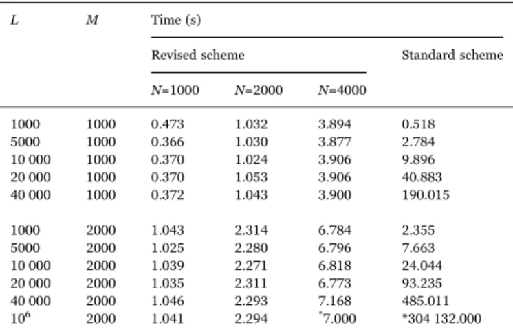
Table 2 shows the time need for updating of both schemes. The most important diﬀerence is that the time need grows quadratically

with L in the standard scheme whereas it is independent from L in the revised scheme. This feature allows us to update the information of millions of observables within seconds in the revised scheme. In contrast to that, an update involvingL = 106_{observables would take}

about four days using the standard scheme. 3.3. Making predictions

Contrary to the revised scheme, making an update with measure-ments in the standard scheme implies computing the predictions of all L observables. As has been shown in the last subsection, updating a large number of observables in the standard scheme is time consuming. However, it is possible to skip the calculation of Ai+1 and to only calculate σ→i+1. Such an incomplete update can be performed much faster than a full update, but without Ai+1 no further updates are possible afterward.

Here, we want to compare the time needs of an incomplete update in the standard scheme (see Eq. (2)) and the prediction of all L observables in the revised scheme (see Eq.(8)with SP=

L L× ). The

timings are reported inTable 3. The number of predicted observables is the same in both schemes. Because experimental information enters an incomplete update (see Eq.(2)), the timings of the standard scheme are also dependent on the number M of measurement points. The time need for a prediction in the revised scheme depends besides L on the number N of model calculations.

As can be seen fromTable 3, the time need for predicting scales linearly with the number L of observables for both schemes. However, comparing the case N=2000 in the revised scheme with the case M=1000 in the standard scheme, the slope of the increase in time need is larger in the standard scheme. Noteworthy, the combined time for an update and a subsequent prediction in the revised scheme is still signiﬁcantly smaller than the time for an incomplete update in the standard scheme.

Finally, we emphasize that it is possible to compute the predictions only for a subset of the observables. This means that the predictions of e.g. 1000 observables can be calculated in about 0.01 s, irrespective of the total number of observables considered in the update procedure. 4. Demonstration

The last section showed that the formulas of the revised scheme can be much faster evaluated than those of the standard scheme. In this section, we provide details about a tentative evaluation of neutron-induced reactions on 181_{Ta using the revised scheme. Especially,}

information needed for updating and predicting was directly retrieved from the outputﬁles of the nuclear model, hence besides→w1and W1no

additional data structures were introduced.

We performed 2000 TALYS[17] calculations with random

varia-Table 2

Comparison of the time need for updating between the revised scheme and the standard scheme as a function of the number L of observables and the number M of measure-ments. In the revised scheme, the time depends also on the number N of model calculations. Numbers with an asterisk are extrapolations.

L M Time (s)

Revised scheme Standard scheme N=1000 N=2000 N=4000 1000 1000 0.473 1.032 3.894 0.518 5000 1000 0.366 1.030 3.877 2.784 10 000 1000 0.370 1.024 3.906 9.896 20 000 1000 0.370 1.053 3.906 40.883 40 000 1000 0.372 1.043 3.900 190.015 1000 2000 1.043 2.314 6.784 2.355 5000 2000 1.025 2.280 6.796 7.663 10 000 2000 1.039 2.271 6.818 24.044 20 000 2000 1.035 2.311 6.773 93.235 40 000 2000 1.046 2.293 7.168 485.011 106 ₂₀₀₀ _1.041 _2.294 *_7.000 _{*304 132.000} Table 3

Comparison of the time need for making predictions between the revised scheme and the standard scheme as a function of the number L of observables. The time need of the revised scheme depends additionally on the number N of model calculations, and those of the standard scheme on the number M of experimental data points. Numbers with an asterisk are extrapolations.

L Time (s)

Revised scheme Standard scheme N=1000 N=2000 M=1000 M=2000 1000 0.008 0.016 0.300 1.794 5000 0.046 0.092 0.639 2.956 10 000 0.095 0.195 1.092 4.491 20 000 0.195 0.397 1.944 7.496 40 000 0.407 1.052 3.645 13.790 106 _14.401 _28.794 *_86.000 *_309.000

(8)

tions of the neutron, proton and alpha optical model parameters. The parameters were sampled uniformly in the range between 80% and 120% relative to their default values. In total, 72 model parameters were adjusted—24 optical model parameters for each particle type. The same grid of 150 incident energies between 1 MeV and 200 MeV was used for all calculations. The calculations were performed on a computer cluster in parallel. TALYS was conﬁgured to provide detailed output, which led to the generation of about 4 × 104_text_{ﬁles in each}

calculation. Theﬁles generated in each calculation required 300 mega-bytes of storage space and contained predictions for about 3 × 106

quantities. Such a number of quantities clearly surpass the domain of application of the standard formulas, especially in the case of stage-wise updates. We bundled the resulting ﬁles of each calculation to a compressed tar archive. Each archive took about 30 megabytes. The total storage requirement for all archives was 60 gigabytes. For updating and making predictions, the relevant ﬁles were extracted whenever needed.

The linear interpolation from the model grid to the experiment grid was directly performed during the process of reading the content of the resultﬁles. In other words, instead of calculating v→k=S(→xk− → )σ0 (see

Eq.(4)), we calculated v→k=S→xk− →Sσ0; and instead of constructing the

sensitivity matrix S and multiplying it with the vectors x→kand σ→0, we

directly interpolated from these vectors. Furthermore, the vectors x→k and σ→0containing the predictions of model calculation never have to be

explicitly constructed because their values are already available in the result files of TALYS. To interpolate a model calculation to an experimental observable, it suffices to locate the two relevant values in the resultfiles. Thus, besides→wi and Wi, only the outputfiles of the model calculations were stored.

It is important to mention that storing the textfiles produced by the model calculations as compressed tar archives is convenient but not efficient. Unpacking and parsing the files introduces a significant overhead to the update procedure. Thus, the time need will be larger than reported in the previous section, where timings were based on an efficient binary representation of the matrix U. However, using directly the outputfiles of TALYS offers great flexibility. In order to introduce a new observable into the update procedure, it suffices to implement a function to read that observable from the TALYS resultfiles.

We performed an update with the experimental data stated in[33]. The 854 experimental data points are distributed over 14 reaction channels. It took about 10 min to evaluate Eqs.(6) and (7). This time span includes unpacking and reading 14files from each of the 2000 archives to construct the matrix V defined in Eq. (4). The update formulas can be evaluated in seconds, hence the overall time need is mainly determined by unpacking and reading thefiles.

The obtained quantities →w1 and W1 enable the computation of

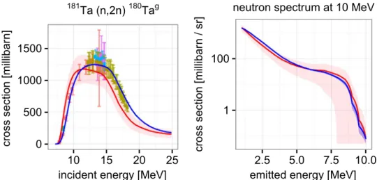
arbitrary observables according to Eq. (8). As an example, we com-puted the evaluated estimates and associated covariances for the (n, 2n)180Tag_{cross section and the neutron spectrum at 10 MeV incident} energy. These cross sections are displayed inFig. 2and their correla-tions in Fig. 3. The computation of the matrix VP _{including the} extraction of 151ﬁles from each tar archive took about 14 min. This example shows that predictions, uncertainties, and correlations can be calculated for any observable predicted by the model in reasonable time.

One might wonder whether the computation of all 3 × 106_evaluated

estimates contained in about 4 × 104_{ﬁles is feasible. To answer this}

question, we computed 45 300 evaluated estimates of emission spectra at different incident energies with the neutron, proton, deuteron, triton, helium-3 nucleus, and alpha nucleus as emitted particles. The computation involves interpolations of the values from 900files from each calculation. Using the already unpackedfiles, the computation of the evaluated estimates required 30 min. Both in terms of number of files and in terms of number of observables, there is about a factor 50 to the computation of all evaluated quantities. Thus, the time needed to obtain the estimates of all 3 × 106_{observables can be estimated to be}

roughly one day. As shown inSection 3.3, using an eﬃcient binary representation, for example in the form of the matrix U, would allow the prediction of all 3 × 106_{observables in about 2 min.}

5. Discussion

The revised scheme presents a fundamentally diﬀerent view on the GLS method than the standard formulas. Rather than updating the values of observables σ→0, one updates a vector of weights w⎯ →⎯0. Each

weight in this vector is associated with a speciﬁc calculation. Similarly, instead of computing all elements of a possible large posterior covariance matrix A1for the observables, one only computes a matrix

W1which contains the covariances between calculations.

The revised scheme clearly demonstrates which information is considered in the update process. The updated quantities→w1and W1

are functions of the results of the model calculations interpolated to the grid of the measurements. Predicted observables not directly related to the measurements play no role in the update process. The information of measurements included in earlier updates aﬀects the current update only through the induced modiﬁcations in w→

0 and W0. It must be

emphasized that the latter two quantities are global information at the level of complete calculations. These two quantities in combination with σ→0 and the model prediction vectors x→k completely specify the current state of knowledge.

One could go even one step further. The information in σ→0and the

model prediction vectors x→kis fully determined by the predictions of a model  performed with some parameter sets{→pk k}=1 ..N. Thus, in principle, it is not necessary to keep the results of model calculations after an update. Required information from model calculations for updating and making predictions can be recomputed at any time. Whether the results of model calculations should be stored or rather recomputed depends on the time requirement of the computation, the size of the output, and the available storage space.

These features allow us to add missing observables at a later point, even if updates have already been performed. In contrast to that, in the standard scheme all relevant observables must be speciﬁed at the very beginning before the generation of the prior. Every eventual measure-ment and any prediction of interest in the future has to be anticipated. If at some point, a prediction of some observable not taken into account is needed, the whole chain from prior generation over updating with measurement data has to be redone.

The increasedﬂexibility in the revised scheme in combination with its speed advantage make it suitable to be implemented as a database application. As has been shown in Section 3.2, the information for millions of observables can be updated in seconds. The predictions of about 106_{observables can be calculated in about 30 s, see}_{Section 3.3}_.

The time need to predict a subset of them, e.g. 1000 observables, is in the order of 0.01 s. These timings were measured on a personal computer. Therefore, these operations could even be performed faster on a server with more powerful hardware, for instance a system where the results of model calculations are distributed over several solid-state drives.

6. Summary and outlook

We presented an alternative computation scheme for the GLS formula which avoids the explicit calculation of the prior covariance matrix and instead works directly with the set of model calculations. The outlined computation scheme is mathematically equivalent to the standard scheme. In typical evaluation scenarios, the feasible number of observables is increased by two or three orders of magnitude compared to the standard scheme. We applied the new scheme in a tentative evaluation of neutron-induced reactions of181Ta involving about 3 × 106_observables.

The revised scheme allows us to add missing observables at a later point, even after updates with experimental data. Updating and making

(9)

predictions are separate processes, and both of these processes can be performed quickly. These features make the revised scheme suited to be implemented as a database application with public access. Users could query evaluated predictions, uncertainties and correlations of any observable which can be predicted by the employed nuclear model. Theﬂexibility of such a database would be a valuable complement to existing data services such as the JEFF or the TENDL library.

Finally, the ability to deal with a large number of observables is a key requirement for the evaluation of high-energy reactions. Evaluated uncertainties may provide essential information for the uncertainty quantiﬁcation of novel technologies, such as the currently planned

MYRRHA reactor and future fusion and transmutation devices. Acknowledgments

We thank Jean-Christoph David and Anthony Marchix for valuable feedback on the paper. This work was performed within the work package WP11 of the CHANDA project (605203) of the European Commission. It is partly based on results achieved within the Impulsprojekt IPN2013-7 ﬁnanced by the Austrian Academy of Sciences and the Partnership Agreement F4E-FPA-168.01 with Fusion for Energy (F4E).

Appendix A. Derivation of the GLS formulas

We derive the GLS formulas by taking recourse to Bayesian statistics (e.g. [40]). An alternative derivation adopting a minimum-variance viewpoint is presented in[4].

Prior knowledge about the true cross section vector→σtrueis speciﬁed in terms of a probability density function (pdf). In the GLS method, this

Fig. 2. Prior cross section (red) and evaluated cross section (blue). The left graph shows the (n,2n) cross section leaving the target nucleus in the ground state. The right graph shows the continuous part of the neutron emission spectrum for incoming neutrons with energy 10 MeV. Depicted data are taken from EXFOR[34]. Original sources are[35,36,37,38,39]. (For interpretation of the references to color in thisﬁgure caption, the reader is referred to the web version of this paper.)

Fig. 3. Change of correlation structure due to updating with experimental data. Both graphs show the correlation between the (n,2n) cross section leaving the target nucleus in the ground state and the emitted neutron spectra for incoming neutrons with energy 10 MeV. The left graph shows the correlations before and the right graph after taking into account experimental data.

(10)

prior pdf is given as a multivariate normal distribution

π0(→ ) ∝ exp{− (→σtrue ₂1 σtrue− → )σ0TA−10 (→σtrue− → )}.σ0 (A.1)

The center vector σ→0and the covariance matrix A0deﬁne its shape.Section 2outlined their determination based on model calculations. We do not

need to know normalization constants in the following discussion.

The dispersion of the measurement vector σ→exp around the true cross section vector is also described by a multivariate normal distribution,

σ σ σ Sσ B σ Sσ

ℓ(→ |→ ) ∝ exp{− (→exp true 1₂ exp− → )trueT −1(→exp− → )}.true _(A.2)

This pdf is called the likelihood. The covariance matrix B reﬂects statistical and systematic errors associated with the measurements. The sensitivity matrix S maps the values of→σtrueto the grid of σ→exp.

Both pdfs can be combined using the Bayesian update formula:

π σ1(→true|→ ) ∝ ℓ(→ |→ )σexp σexpσtrue π0(→ ).σtrue (A.3)

The posterior pdfπ1represents an improved knowledge about→σtrue. The exponents of both prior pdf and likelihood are quadratic forms with respect

to→σtrue. The exponent of the posterior is the sum of the exponents of the prior pdf and the likelihood and therefore also a quadratic form. Thus, the

posterior pdf is a multivariate normal distribution,

π σ1(→ ) ∝ exp{− (→true ₂1 σtrue− →)σ1TA1−1(→σtrue− →)}.σ1 (A.4)

The center vector→σ1and the covariance matrix A1can be determined by comparing the exponents of the left and right hand side of Eq.(A.3):

σ σ σ σ σ σ σ σ σ σ σ σ σ σ σ σ C σ σ σ σ σ σ σ σ A A A A A A A A S B S S B B S B → → _{+ →} _{→ + →} → _{+ →} _{→ = →} → _{+ →} _{→ + →} → _{+ →} _{→ + →} → _{+ →} → + → → + → → . T T T T T T T T T _T T _T T T

true 1−1 true true 1−1 1 1 1−1 true 1 1−1 1 true 0−1 true true −10 1 0 0−1 true 0 −10 0 true −1 true true −1 exp

exp −1 true exp −1 exp (A.5)

Using normalized pdfs for the prior and the likelihood, the Bayesian update formula yields a normalized posterior pdf. Terms independent of→σtruein

the exponents of the pdfs only aﬀect the normalization constant. Therefore, the sides of Eq.(A.5)are allowed to diﬀer by a constant C and we only have to consider terms with→σtrue. Matching the terms with→σtrueof the left and right hand side of Eq.(A.5)leads to

A =A +S B ST 1 −1 0 −1 −1 _(A.6) σ σ σ A → =A → +S BT → 1 −1 1 0−1 0 −1 exp (A.7)

Applying the Woodbury matrix identity for inversion[41], the posterior covariance matrix can be expressed as

A =A −A S SA ST( T+B) SA .

1 0 0 0 −1 0 (A.8)

Multiplying Eq.(A.7)from the left with this representation of A1yields σ σ A S SA S B Sσ A S B SA S B SA S B σ

→ = → − T( T+ ) → + T( − ( T+ ) T )→

1 0 0 0 −1 0 0 −1 0 −1 0 −1 exp (A.9)

We rearrange the bracketed expression in the second line:

B−1− (SA ST+B) SA S BT = (SA ST+B) ((SA ST+B B) −SA S BT ) = (SA ST+B) .

0 −1 0 −1 0 −1 0 −1 0 −1 0 −1 (A.10)

Using this identity, we can write Eq.(A.9)as

σ σ A S SA S B σ Sσ

→ = → + T( T+ ) (→ − → ).

1 0 0 0 −1 exp 0 (A.11)

Eqs.(A.8) and (A.11)are theﬁnal forms of the GLS formulas as stated in Eqs.(2) and (3).

References

[1] NEA, Uncertainty and Target Accuracy Assessment for Innovative Systems Using Recent Covariance Data Evaluations, NEA/OECD, Paris, 2008.

[2] A.J. Koning, D. Rochman, Towards sustainable nuclear energy: putting nuclear physics to work, Ann. Nucl. Energy 35 (11) (2008) 2024–2030.http://dx.doi.org/ 10.1016/j.anucene.2008.06.004.

[3] D. Rochman, A.J. Koning, S.C. van der Marck, A. Hogenbirk, D. van Veen, Nuclear data uncertainty propagation: total Monte Carlo vs. covariances, J. Korean Phys. Soc. 59 (23) (2011) 1236.http://dx.doi.org/10.3938/jkps.59.1236.

[4]D.W. Muir, Evaluation of correlated data using partitioned least squares: a minimum-variance derivation, Nucl. Sci. Eng. 101 (1) (1989) 88–93. [5] T. Kawano, K. Shibata, Covariance Evaluation System, Technical Report

JAERI-Data/Code 97-037, JAERI, Japan, 1997.

[6]D. Smith, L.A. Naberejnev, Large Errors and Severe Conditions (2002). [7] M. Herman, P. Oblozinsky, D. Rochman, T. Kawano, L. Leal, Fast Neutron

Covariances for Evaluated Data Files, Technical Report BNL-75893-2006-CP, Brookhaven National Laboratory, May 2006.

[8] E. Bauge, S. Hilaire, P. Dossantos-Uzarralde, Evaluation of the Covariance Matrix of Neutronic Cross Sections with the Backward–Forward Monte Carlo Method, EDP Sciences, Les Ulis, France; London, UK, 2007.http://dx.doi.org/10.1051/ ndata:07339.

[9] H. Leeb, D. Neudecker, T. Srdinko, Consistent procedure for nuclear data evaluation based on modeling, Nucl. Data Sheets 109 (12) (2008) 2762–2767.

http://dx.doi.org/10.1016/j.nds.2008.11.006.

[10] D.L. Smith, A uniﬁed Monte Carlo approach to fast neutron cross section data evaluation, in: Proceedings of the 8th International Topical Meeting on Nuclear Applications and Utilities Of Accelerators, Pocatello, July 2008, pp. 736–743. [11] D. Neudecker, The full Bayesian evaluation technique and its application to

isotopes of structural materials (Ph.D. thesis), Technische Universität Wien, Austria, 2012.

[12] R. Capote, D.L. Smith, A. Trkov, M. Meghzifene, A new formulation of the uniﬁed Monte Carlo approach (UMC-B) and cross-section evaluation for the dosimetry reaction55_Mn(n,g)56_{Mn, J. ASTM Int. 9 (3) (2012) 104115.}_{http://dx.doi.org/}

10.1520/JAI104115.

[13] A.J. Koning, Bayesian Monte Carlo method for nuclear data evaluation, Nucl. Data Sheets 123 (2015) 207–213.http://dx.doi.org/10.1016/j.nds.2014.12.036. [14] R. Capote, D. Smith, A. Trkov, Nuclear data evaluation methodology including

estimates of covariances, EPJ Web Conf. 8 (2010) 04001.http://dx.doi.org/10. 1051/epjconf/20100804001.

[15] G. Schnabel, Large scale Bayesian nuclear data evaluation with consistent model defects (Ph.D. thesis), Technische Universitat Wien, Vienna, 2015. URL〈http:// katalog.ub.tuwien.ac.at/AC12392895〉.

[16] A.J. Koning, S. Hilaire, M.C. Duijvestijn, TALYS-1.0, EDP Sciences, Les Ulis, France; London, UK, 2007.http://dx.doi.org/10.1051/ndata:07767. [17] A.J. Koning, S. Hilaire, S. Goriely, TALYS-1.6– A Nuclear Reaction Program

(December) (2013)〈http://www.talys.eu〉.

[18] D.W. Muir, A. Trkov, I. Kodeli, R. Capote, V. Zerkin, The Global Assessment of Nuclear Data, GANDR, EDP Sciences, Les Ulis, France; London, UK, 2007.http:// dx.doi.org/10.1051/ndata:07635.

[19] International AtomicEnergy Agency. URL〈https://www.iaea.org/〉.

(11)

[20] G. Schnabel, H. Leeb, A. New, Module for large scale Bayesian evaluation in the fast neutron energy region, Nucl. Data Sheets 123 (2015) 196–200.http://dx.doi.org/ 10.1016/j.nds.2014.12.034.

[21] Nuclear Energy Agency– JEFF and EFF Projects. URL 〈https://www.oecd-nea. org/dbforms/data/eva/evatapes/jeﬀ_32/〉.

[22] A. Koning, D. Rochman, J. Kopecky, J. Sublet, M. Fleming, E. Bauge, S. Hilaire, P. Romain, B. Morillon, H. Duarte, S. van der Marck, S. Pomp, H. Sjostrand, R. Forrest, H. Henriksson, O. Cabellos, S. Goriely, J. Leppanen, H. Leeb, A. Plompen, R. Mills, TENDL-2015 Nuclear Data Library. URL〈https://tendl.web.psi.ch/tendl_ 2015/tendl2015.html〉.

[23] G. Evensen, Sequential data assimilation with a nonlinear quasi-geostrophic model using Monte Carlo methods to forecast error statistics, J. Geophys. Res. 99 (C5) (1994) 10143.http://dx.doi.org/10.1029/94JC00572.

[24] G. Evensen, Data Assimilation: The Ensemble Kalman Filter, 2nd ed., Springer, Dordrecht, 2009.

[25] H. Matthies, G. Strang, The solution of nonlinearﬁnite element equations, Int. J. Numer. Methods Eng. 14 (11) (1979) 1613–1626.http://dx.doi.org/10.1002/ nme.1620141104.

[26] J. Nocedal, Updating quasi-Newton matrices with limited storage, Math. Comput. 35 (151) (1980) 773.http://dx.doi.org/10.2307/2006193.

[27] A.J. Koning, J.P. Delaroche, Local and global nucleon optical models from 1 keV to 200 MeV, Nucl. Phys. A 713 (3–4) (2003) 231–310.http://dx.doi.org/10.1016/ S0375-9474(02)01321-0.

[28] A.J. Koning, Bayesian Monte Carlo method for nuclear data evaluation, Eur. Phys. J. A 51(12) (2015).http://dx.doi.org/10.1140/epja/i2015-15184-x.

[29] D. Smith, N. Otuka, Experimental nuclear reaction data uncertainties: basic concepts and documentation, Nucl. Data Sheets 113 (12) (2012) 3006–3053.

http://dx.doi.org/10.1016/j.nds.2012.11.004.

[30] R Development Core Team, R: A Language and Environment for Statistical Computing, R Foundation for Statistical Computing, Vienna, Austria, 2008 (ISBN 3-900051-07-0). URL〈http://www.R-project.org〉.

[31] OpenBLAS: An Optimized BLAS Library〈http://www.openblas.net/〉.

[32] M.J. Kane, J. Emerson, S. Weston, Scalable strategies for computing with massive data, J. Stat. Softw. 55 (14) (2013) 1–19 (URL 〈http://www.jstatsoft.org/v55/i14/

〉).

[33] H. Leeb, G. Schnabel, T. Srdinko, V. Wildpaner, Bayesian evaluation including covariance matrices of neutron-induced reaction cross sections of181_{Ta, Nucl. Data} Sheets 123 (2015) 153–158.http://dx.doi.org/10.1016/j.nds.2014.12.027. [34] N. Otuka, E. Dupont, V. Semkova, B. Pritychenko, A. Blokhin, M. Aikawa,

S. Babykina, M. Bossant, G. Chen, S. Dunaeva, R. Forrest, T. Fukahori, N. Furutachi, S. Ganesan, Z. Ge, O. Gritzay, M. Herman, S. Hlavač, K. Katō, B. Lalremruata, Y. Lee, A. Makinaga, K. Matsumoto, M. Mikhaylyukova, G. Pikulina, V. Pronyaev, A. Saxena, O. Schwerer, S. Simakov, N. Soppera, R. Suzuki, S. Takács, X. Tao, S. Taova, F. Tárkányi, V. Varlamov, J. Wang, S. Yang, V. Zerkin, Y. Zhuang, Towards a more complete and accurate experimental nuclear reaction data library (EXFOR): international collaboration between Nuclear Reaction Data Centres (NRDC), Nucl. Data Sheets 120 (2014) 272–276.http:// dx.doi.org/10.1016/j.nds.2014.07.065.

[35] F. Peiguo, Chin. J. Nucl. Phys. 7 (3) (1985) 242.

[36] L. Han-Lin, Z. Wen Rong, F.P. Guo, Measurement of the neutron cross sections for the reactions169_{(n, 2n)}168_Tm,169_Tm(n,3n)167_{Tm, and}181_Ta(n,2n)180m_{Ta, Nucl.} Sci. Eng. 90 (3) (1985) 304–310.http://dx.doi.org/10.13182/NSE85-3. [37] A.A. Filatenkov, Leningrad Reports, Technical Report 258, Khlopin Radium

Institute, 2001.

[38] C. Zhu, Y. Chen, Y. Mou, P. Zheng, T. He, X. Wang, L. An, H. Guo, Measurements of (n, 2n) reaction cross sections at 14 MeV for several nuclei, Nucl. Sci. Eng. 169 (2) (2011) 188–197.http://dx.doi.org/10.13182/NSE10-35.

[39] C. Bhatia, M.E. Gooden, W. Tornow, A.P. Tonchev, Ground-state and isomeric-state cross sections for181_Ta(n,2n)180_{Ta between 8 and 15 MeV, Phys. Rev. C 87(3)} (2013).http://dx.doi.org/10.1103/PhysRevC.87.031601.

[40] E.T. Jaynes, Probability Theory: The Logic of Science, Cambridge University Press, Cambridge, UK; New York, NY, 2003.

[41] M.A. Woodbury, Inverting Modiﬁed Matrices, Statistical Research Group, Memo. Rep. no. 42, Princeton University, Princeton, N.J., 1950.