Design of a top-down computer vision algorithm dedicated to the recognition of cortical sulci

(1)

HAL Id: tel-02325893

https://tel.archives-ouvertes.fr/tel-02325893

Submitted on 22 Oct 2019

HAL is a multi-disciplinary open access archive for the deposit and dissemination of sci-entific research documents, whether they are pub-lished or not. The documents may come from teaching and research institutions in France or abroad, or from public or private research centers.

L’archive ouverte pluridisciplinaire HAL, est destinée au dépôt et à la diffusion de documents scientifiques de niveau recherche, publiés ou non, émanant des établissements d’enseignement et de recherche français ou étrangers, des laboratoires publics ou privés.

dedicated to the recognition of cortical sulci

Leonie Borne

To cite this version:

Leonie Borne. Design of a top-down computer vision algorithm dedicated to the recognition of cortical sulci. Medical Imaging. Université Paris Saclay (COmUE), 2019. English. �NNT : 2019SACLS322�. �tel-02325893�

(2)

Th

`ese

de

doctor

at

NNT

:

2019SA

CLS322

Conception d’un algorithme de vision par

ordinateur ”top-down” d édi é à la

reconnaissance des sillons corticaux

Th èse de doctorat de l’Universit é Paris-Saclay pr épar ée à l’Universit é Paris-Sud Ecole doctorale n◦_{575 Electrical, Optical, Bio: Physics and Engineering (EOBE)}

Sp écialit é de doctorat : Imagerie et physique m édicale

Th èse pr ésent ée et soutenue à Saclay, le 01/10/2019, par

L ´

EONIE

B

ORNE

Composition du jury :

Isabelle Bloch

Professeur, T ´el ´ecom Paris-Tech, Univ. Paris-Saclay (LTCI)

Pr ´esidente Pierrick Coup ´e

Charg ´e de recherche, CNRS, Univ. Bordeaux (LABRI)

Rapporteur Franc¸ois Rousseau

Professeur, INSERM, IMT Atlantique (LaTIM)

Rapporteur Arnaud Cachia

Professeur, CNRS, Univ. Paris-Descartes (LaPsyD ´E)

Examinateur Olivier Coulon

Directeur de Recherche, CNRS, Univ. Aix-Marseille (INT)

Examinateur Mark Jenkinson

Professeur, Univ. Oxford (FMRIB)

Examinateur Jean-Franc¸ois Mangin

Directeur de recherche, CEA, Neurospin (UNATI)

Directeur de th `ese Denis Rivi `ere

Charg ´e de recherche, CEA, Neurospin (UNATI)

(3)

Doctor

al

thesis

NNT

:

2019SA

CLS322

algorithm dedicated to the recognition of

cortical sulci

PhD thesis of University Paris-Saclay prepared at University Paris-Sud Doctoral school n◦575 Electrical, Optical, Bio: Physics and Engineering (EOBE)

PhD speciality : Imaging and Medical Physics

Thesis presented and defended in Saclay, on October, 1st_{, 2019, by}

L ´

EONIE

B

ORNE

Composition of the jury :

Isabelle Bloch

Professor, T ´el ´ecom Paris-Tech, Univ. Paris-Saclay (LTCI)

President of the jury Pierrick Coup ´e

Professor, CNRS, Univ. Bordeaux (LABRI)

Reviewer Franc¸ois Rousseau

Professor, INSERM, IMT Atlantique (LaTIM)

Reviewer Arnaud Cachia

Professor, CNRS, Univ. Paris-Descartes (LaPsyD ´E)

Examiner Olivier Coulon

Research director, CNRS, Univ. Aix-Marseille (INT)

Examiner Mark Jenkinson

Professor, Univ. Oxford (FMRIB)

Examiner Jean-Franc¸ois Mangin

Research director, CEA, Neurospin (UNATI)

Supervisor Denis Rivi `ere

(4)

Acknowledgements

To Nicolas, who had not chosen to do a thesis, but who still experienced it by proxy. Thank you for supporting me, feeding me and taking me out even when it was raining.

To Denis, for his availability, his attentive ear and for showing me the plea-sures of research and of Parisian subsoils. Thank you for these cata-ptivating experiences!

To Jean-Fran¸cois, for his support, encouragement and eternal optimism throughout this thesis. Thank you for being so for both of us.

To my colleagues for their help, whatever the solicitation, the discussions in the canteen, the cakes in the office that never stayed very long and the Chilean parties. Thank you for being there, simply.

To my running colleagues, for our discussions, our shared sweat, our cheesy evenings and our wild weekend with the plastic chicken. Thank you for your good humour at all times.

To my whole family, for their support and constant interest in my research, although I doubt I have been able to explain it properly. Thank you for your encouragement, from the very beginning.

Thank you to all of you without whom this thesis would not have been such an enriching experience, in discovery, knowledge and encounter.

(5)

(6)

Introduction

Context

Considered as the seat of our intelligence, the brain is currently one of the most challenging enigmas that remains to be solved. Its function and in particular its dysfunctions fascinate. The link between the anatomy of the brain and its function is one of the unknowns of this enigma. For a while, it was common to think that our ability to calculate was related to the size of a bump in our cranium box: the ”math bump”. This expression comes from a pseudoscience, the phrenology, which was very popular in the 19th century. This pseudoscience attributed each aspect of an individual’s personality to the extent of a bump in the cranium. Of course, the shape of the skull is not linked to that of the brain and this pseudoscience no longer has any credit. However, it has been shown that calculation actually involves specific areas of our brain, whose location is relatively stable from one individual to another. In fact, the appearance of non-invasive imaging, such as Magnetic Resonance Imaging (MRI), about 40 years ago allowed us to visualize the brain, first anatomically and then functionally. So is the functioning of these areas related to the anatomical organization of the brain? Regarding the anatomy of the brain’s surface, the most noticeable feature is its convolutions, which are so variable that each individual has unique fold patterns. However, this striking feature is still poorly understood today.

From a Darwinian point of view, these folds are considered as a trick of evolution to increase the cortical surface without modifying the volume of the cranial cavity. Thus, the degree of folding, the complexity of their arrangement and their variability seem to be related to the degree of in-telligence of each species. Indeed, most animals have a smooth brain, only some mammals, such as great apes (but also ferrets, cats, dogs, horses, cows, elephants, etc.), and some cetaceans, such as dolphins, have a folded brain. Note that some cetaceans have a brain with a volume and degree of folding greater than ours, which suggests a much higher degree of intelligence! This observation nevertheless shows the importance of folds in the uniqueness of the human species.

(11)

pregnancy and the sulci do not change their overall configuration afterwards. This period also corresponds to the emergence of cortical architecture: the migration of neurons into different predefined areas occurs just before the formation of folds. This observation suggests a link between cortical folds and the functional organization of the cortex. In fact, unusual fold patterns are generally linked to abnormal developments that can lead to psychiatric syndromes such as epilepsy or schizophrenia. Moreover, a close link has been demonstrated between the shape of certain sulci and cognitive func-tions such as manual laterality or reading. Therefore, the fold patterns appear to be signatures of each individual’s functional organization. This hypothesis is now relatively accepted for the most important sulci but is more controversial for secondary sulci.

Anyway, the study of cortical folds requires a high level of expertise that few neuroanatomists have at this time. In order to facilitate their study, artificial intelligence algorithms are used in this thesis to automate tasks requiring advanced learning. But how do you teach a task to an algorithm? This question is addressed by a field of study of artificial intelligence: the machine learning. This approach is inspired by our own way of learning: for exemple, learning to read involves teaching based on decoding many words and texts. Similarly, machine learning algorithms ”learn” from data. Today, artificial intelligence has made significant progress, especially in the field of computer vision, which is revolutionizing our daily lives. This is due to the emergence of a new method inspired by the brain function: the deep learning. This technique has allowed smartphones to talk, computers to beat chess champions, cars to drive on their own, etc. Will they also allow us to decipher our sulcal lines?

Challenges

The first challenge addressed during this thesis is the automation of local fold pattern classification. Based on a pattern identified by experts, the ob-jective is to automate its recognition, which raises several issues. First, the distinction of patterns is sometimes difficult to the naked eye and requires ad-hoc criteria. Second, due to the extreme variability of cortical folds, the choice of classifier is a crucial step. Third, as we are interested in local pat-terns, the classifier must be able to handle particularly noisy data. Fourth, since manual labeling is time-consuming, the available learning databases are limited in size and can be largely unbalanced if the pattern is rare.

The second challenge concerns the automation of cortical sulci labeling. In order to study the geometry of cortical folds, neuroanatomists have at-tempted to define a sulci dictionary to differentiate these structures. Among the several proposed nomenclatures, the main sulci generally have a com-mon label, but the fold variability is so high that there is no consensual

(12)

Contents 3

nomenclature for all sulci. However, whatever the nomenclature used, sulci labeling is generally tedious and requires a long expertise in the field. Thus, the automation of sulci recognition is essential to enable large-scale studies. This challenge has already been addressed several times, including in the lab-oratory hosting this thesis, but the results obtained are not yet satisfactory, on the one hand because the recognition rates are too low to reproduce the observations obtained with manual labeling and on the other hand because the recognition pipeline is dependent on an error-prone sub-segmentation process.

Thesis organization

This thesis is organized in two parts. The first part gives a state of the art on the topic under study (i.e. cortical sulci) and on the methods of medical image analysis on which the work of this thesis is based (i.e. multi- atlas segmentation techniques and convolutional neural networks). The second part presents the methods implemented for the automatic classification of local fold patterns and the automatic labeling of the sulci themselves. For these two problems, several methods are compared and the best method obtained is tested in practice.

Thesis contribution

The work carried out during this thesis has led to the emergence of two types of tools dedicated to the study of cortical folds, which will soon be available in the BrainVISA/Morphologist toolbox (http://brainvisa.info). The first tool automates the classification of local cortical fold patterns. This issue had never been addressed before. The second tool automates sulci labeling by eliminating the main defects of the model previously proposed by the BrainVISA/Morphologist toolbox. Thus, in addition to improving perfor-mance and speed, the proposed new model is robust to sub-segmentation errors, which is one of the greatest weaknesses of the old system.

This thesis continues the work of J.-F. Mangin (Mangin, 1995), D. Rivière (Riviere, 2000) and M. Perrot (Perrot, 2009) during their respective the-ses. It took place within the NAO (Neuroimagerie Assistée par Ordinateur ) team of the Neurospin laboratory at CEA (Commissariat à l’énergie atom-ique et aux énergies alternatives) in Saclay. The work has benefit from an outstanding visualization environment provided by the Simulation house in order to manipulate and visualize hundreds of brains simultaneously (http://maisondelasimulation.fr).

(13)

(14)

Part I

(15)

(16)

Chapter 1 Cortical sulci

Abstract

The complex and diverse arrangement of cortical folds is the most striking, interesting and yet poorly understood coarse morphological feature of the human brain. First, what is a sulcus? To answer this question, I will briefly review the anatomy of the brain in order to understand the place of sulci in its organization. Second, why study sulci? To understand the interest aroused by cortical folds, I will focus on their anatomy and its main components before presenting the mechanism of fold formation and their link with the functional organization of the brain. Third, how to study sulci? The choice of the fold representation is a key step for studying these structures. I will make a quick overview of the different representations used so far before developing the one used in this thesis.

1.1 Brain anatomy

Let’s do a quick reminder about the anatomy of the human brain.

On a cellular scale, the brain is composed of nerve cells, called neurons, and glial cells. Neurons transmit information in the form of nerve impulses, while glial cells nourish, support and protect neurons. Glial cells also seem to have a significant, but still poorly understood, role in brain function. In order to communicate with each other, neurons have two types of extensions: dendrites that collect nerve impulses and carry them to the cell body, and the axon, a long fiber that carries information to other neurons.

On an anatomical scale, the cerebrum represents the largest part of the human brain. It is separated into two hemispheres communicating through the corpus callosum. Several brain nuclei are located in the centre of the brain: the central grey nuclei, the thalamus and the hypothalamus. Also in the center of the brain, there are cavities filled with cerebrospinal fluid: the ventricles. Finally, the cerebellum is below the rest of the brain.

(17)

The cellular bodies of cerebrum neurons are located either on the pe-riphery where they form a grey layer, the cortex, or in nuclei buried in the depths of the brain. The axons form clusters of fibers, which constitute the white matter. In this thesis, we focus on a particular region of the brain, the cortex, which is supposed to be the seat of high-level functions.

1.2 Sulci: anatomy, formation and link with

func-tional organization

1.2.1 Sulci and gyri anatomy

The cortex is divided into several convolutions, called gyri, delimited by folds, called sulci. On a larger scale, these structures are grouped into several large cortical lobes on each hemisphere, generally delimited by large deep sulci (Figure 1.1). Indeed, the central sulcus separates the frontal lobe from the parietal lobe; the parieto-occipital fissure separates the occipital lobe from the parietal lobe; the cingulate sulcus separates the frontal lobe from the limbic lobe on the inner side, etc. There is also a buried lobe at the bottom of the sylvian valley, between the temporal and frontal lobes: the insula.

Figure 1.1 – Four main cortical lobes. (Miller and Cummings, 1999) In order to study cortical folds, neuroanatomists have sought to asso-ciate a name to each sulcal or gyral structure, which has led to the emer-gence of several nomenclatures such as those described by Ono et al. (1990), Rademacher et al. (1992), Destrieux et al. (2010), etc. However, applying one of these nomenclatures, designed on a limited number of brains, to the

(18)

Sulci: anatomy, formation and link with functional organization9

thousands of brains now available is much more complicated than expected. In fact, the folds are so variable that the labeling of a sulcus, even a pri-mary one, can raise many questions. Note that if among the nomenclatures proposed so far, none of them is a consensus in the community, it is also because of the extreme variability of these structures.

1.2.2 Mechanism at the origin of cortical folds

Cortical folds appear during the third trimester of pregnancy. Once formed, their shape may vary slightly depending on the environment and the age of the subject. However, they maintain roughly the same configuration, which makes them excellent markers of early brain development. Nevertheless, the mechanism behind the formation of folds is not yet fully understood. Recently, a multicultural community has begun to focus on modeling the mechanisms that drive the folding process.

From a physical point of view, it has been demonstrated that the me-chanical instability induced by the tangential expansion of the grey matter of the cortex is sufficient to simulate the folding process (Tallinen et al., 2014, 2016) (Figure 1.2). This result is a big step forward, but this modeling does not seem sufficient to obtain realistic folding patterns.

Figure 1.2 – Simulation of uniform tangential expansion of the cortical layer from a smooth fetal brain. This expansion is sufficient to reproduce the cortex gyrification process. (Tallinen et al., 2016)

Two other major hypotheses exist to explain the mechanism of sulci formation.

The first hypothesis is based on the relationship between folding and the existence of primary molecular maps, called protomaps (Fern´andez et al., 2016). These maps, supposed to be the result of heterogeneous gene expres-sion, are present before the neuronal migration accompanying the construc-tion of the cortex, followed by its folding. The existence of a ”protomap” of the primary folding scheme is now relatively accepted (de Juan Romero et al., 2015). Thus, the areas of the protomap intended to become gyri

(19)

would present an increased multiplication of neurons, explaining the expan-sion maxima responsible for the formation of ”bumps”. Therefore, the me-chanical model mentioned above could be improved by taking into account this protomap model.

The second hypothesis, compatible with the first, is that slight fibre ten-sions could play a role (Van Essen, 1997). After the appearance of primary sulci, these tensions could explain the following dynamic steps forming the secondary and tertiary folds. However, this hypothesis is far from being accepted.

The appearance of cortical folds is concomitant with the distribution of the cortex into different functional areas (Kostovic and Rakic, 1990; Sur and Rubenstein, 2005; Reillo et al., 2010). Is that a coincidence? I will discuss the links between folding patterns and functional organization in the next section.

1.2.3 Relations with cortical functional organization

The cortex is often divided into several zones, each supposed to be special-ized in a different cognitive function (Amunts and Zilles, 2015; Glasser et al., 2016). The existence of close links between primary sulci and functional ar-chitecture is generally accepted (Welker, 1990; Fischl et al., 2007). These links are more controversial for other sulci, where the number of studies re-porting similar results is very low (Watson et al., 1993; Amiez et al., 2006; Weiner et al., 2014). However, if we consider anatomical studies that are not based on a functional investigation, several of them suggest a much closer link than what has been demonstrated today.

1.2.3.1 Abnormal fold patterns and psychiatric pathologies Abnormal folds patterns are usually related to anomalies in early brain de-velopment. For example, in (B´en´ezit et al., 2015), the abnormal development of interhemispheric fibres strongly disrupts the folding process.

Less obvious links have been identified with some neurodevelopmental diseases. For example, epilepsy is often due to incomplete migration of a group of neurons trapped in the white matter before reaching the cortical mantle: this group is called focal cortical dysplasia. This dysplasia is some-times linked to abnormal fold patterns (Besson et al., 2008; R´egis et al., 2011; Mellerio et al., 2014; Roca et al., 2015), even when the dysplasia is invisible on MRI (Figure 1.3).

Similarly, a link has been established between the patterns of the cin-gulate sulcus and schizophrenia. The shape of this sulcus can be catego-rized into two patterns: the single type and the double parallel type (Fig-ure 1.4). It has been shown that patients with schizophrenia tend to have

(20)

Sulci: anatomy, formation and link with functional organization11

Figure 1.3 – The Power Button Sign: a fold pattern related to epilepsy. (Mellerio et al., 2014).

more symmetric patterns (same pattern on each hemisphere) than controls (Le Provost et al., 2003; Y¨ucel et al., 2003).

It is interesting to note that children with the same lack of asymme-try have poor inhibitory control (Borst et al., 2014; Cachia et al., 2014). Thus, the study of folding patterns is not limited to psychiatric diseases but extends to the functioning of normal brains.

1.2.3.2 Sulci shape and brain function

In addition to studies based on fold patterns, other anatomical studies are based on a comparison of sulci length and depth between two groups of subjects (Mangin et al., 2010; Alem´an-G´omez et al., 2013; De Guio et al., 2014; Janssen et al., 2014; Hamelin et al., 2015; Leroy et al., 2015; Muellner et al., 2015). These studies show that the links between function and sulci shape can be much more subtle than an abnormal pattern.

Consider the example of the central sulcus. It is commonly accepted that this sulcus delimits the primary motor cortex of the primary somatosensory cortex. This special position makes it a particularly interesting structure to study. Indeed, it has been shown that the shape of this sulcus is related to manual laterality (Sun et al., 2012) and recovery after a subcortical stroke (Jouvent et al., 2016). The link between its form and functional organiza-tion was also studied through funcorganiza-tional MRI activaorganiza-tions: Sun et al. (2016) shows that the position of the ”hand knob” is related to the hand’s motor activation, as well as to the premotor linguistic zone.

Therefore, studies on the geometry of cortical folds reveal links with the functional organization of the brain. However, these studies would not have

(21)

Figure 1.4 – Two folding patterns identified in the cingulate region. (Cachia et al., 2014)

been possible without representing in 3D the folds from the MRI acquisition, allowing for example to facilitate their visualization when defining patterns or to evaluate the characteristics of a sulcus (length, depth, opening, etc).

1.3 Sulci representation

In the literature, there are many different approaches for representing corti-cal folds, each with its advantages and disadvantages. In this thesis focusing on the classification of local fold patterns and on the sulci labeling, the rep-resentation chosen must be sufficiently exhaustive to allow the distinction of these complex structures while remaining standardized enough to be gener-alizable.

Therefore, in this section, I will give a quick overview of the representa-tions of sulci presented in the literature, before developing the representation used in this thesis.

1.3.1 Overview

When considering cortical folds, two types of representations are possible: either the representations of bumps (gyri) or those of hollows (sulci).

(22)

Sulci representation 13

The first type of representation, used for example by Fischl et al. (2004) and Chen et al. (2017), is based on a labelisation of the cortical surface into different gyri. These representations are probably more appropriate when considering functional MRI or diffusion MRI. In fact, white matter fibers appear to preferentially fan out in gyri (Van Essen, 1997), so there is a high probability that this is where the functional activity is also concentrated. However, gyri do not have a well delineated boundary and are generally defined by the sulci surrounding them.

Therefore, the second type of representation, based on sulci, is more obvious from an anatomical point of view because they are better defined structures. As the representation used in this thesis is based on sulci, I will develop in particular this type of representation below.

1.3.1.1 Sulcus regions

As for gyri representation, this representation of sulci is based on the cortical surface labelisation. Each sulcus is represented by a sulcus region, i. e. the surface of the cortex that surrounds the sulci (Behnke et al., 2003; Rettmann et al., 2005; Vivodtzev et al., 2006; Yang and Kruggel, 2009).

This representation is particularly effective in capturing all variations of cortical surface depth, including dimples. However, it is not ideal for repre-senting the 3D layout of these structures. Moreover, it takes into account the sulci’s opening, which is highly dependent on the subject’s age. Other representations allow better normalization of the data.

1.3.1.2 Sulcus roots/pits

In order to overcome the high variability of folds, it was proposed to focus on sulcus roots, also called sulcus pits. These structures, corresponding to local maximum depths, represent the position of the first folds during their formation in utero. Their selection is supposed to provide more information on the architectural organization of the cortex (R´egis et al., 2005; Lohmann et al., 2007; Im et al., 2009; Mangin et al., 2015a; Im and Grant, 2019).

However, these approaches represent the sulci by a set of points where only critical parts of the structure shape are preserved, which is not appro-priate for our applications.

1.3.1.3 Sulcus bottom lines

In the late 1990s, the use of pipelines representing the cortical surface, no longer in 3D, but as a 2D spherical surface (Dale et al., 1999), promoted surface representations of sulci. These surface representations are based on the sulci bottom line as it is more accessible once the cortical surface is represented by a 2D mesh (Kao et al., 2007; Shi et al., 2008; Li et al., 2010; Shattuck et al., 2009; Seong et al., 2010; Lyu et al., 2018).

(23)

Although this representation is more appropriate than sulcal roots for sulci labeling, it does not consider information related to the deep extension of sulci. Yet, knowing the depth or inclination helps to recognize some sulci: for example, primary sulci are deeper than others, collateral sulcus has a characteristic inclination, etc.

1.3.1.4 Sulcus segments

When sulci are considered as hollows filled with cerebrospinal fluid, they can be extracted by making a negative mold of the cortical surface. To avoid representing the sulci opening, the extracted structure can be displayed by median surfaces between the two walls surrounding each sulcus. These median surfaces are then divided into several sulcus segments, also called elementary folds.

Compared to sulcus bottom lines, the sulcus segments are particularly interesting for representing information related to the deep extension of sulci. Two representations are based on this notion of sulcus segments. The first representation corresponds to smooth structures, called sulcus rib-bons, which do not represent the branches of sulci (Le Goualher et al., 1997; Vaillant and Davatzikos, 1997; Zeng et al., 1999; Zhou et al., 1999). The second representaion corresponds to the interface between the two walls bor-dering the sulci (Mangin, 1995; Le Goualher et al., 1998; Riviere et al., 2002; Klein et al., 2005; Perrot et al., 2011). By displaying branches of sulci, this representation is therefore much more suitable for studying local patterns of cortical folds. Thus, this more exhaustive representation has been used in this thesis.

1.3.2 Morphologist/BrainVISA representation

The Morphologist pipeline of the BrainVISA toolbox provides a represen-tation of sulcus segments taking into account the branches of sulci (Rivi`ere et al., 2009). This pipeline, first described in (Mangin et al., 1995), then more recently in (Riviere et al., 2002) and (Mangin et al., 2004), constitutes the preprocessing, allowing the extraction of sulci, used in this thesis. It consists of four major steps: first, the segmentation of white and grey mat-ter from MRI, then the extraction of the skeleton of cortical folds, followed by its division into elementary folds and finally the representation of these folds as a graph (Figure 1.5).

• White/grey matter segmentation: First, MRIs are analyzed to segment white matter and grey matter. To do this, a bias correction is made to eliminate signal intensity inhomogeneities depending on spatial position due to weaknesses in the acquisition process. Then, the intensity distribution is analyzed to detect grey and white matter, whose intensities vary according to the MR sequence and the subject.

(24)

Figure 1.5 – A computer vision pipeline mimicking a human anatomist (Man-gin et al., 2015b). A: interface between the cerebral envelope and the cortex. B: interface between white matter and grey matter. C: extraction of the fold skeleton. D: cutting of the skeleton into elementary folds. E: Folds labeling using the model of Perrot et al. (2011)

Finally, by using the histogram produced, the image is binarized by keeping the range of intensities that can belong to the brain. The binary image is eroded iteratively until a seed is obtained which is then dilated to form the shape of the brain.

• Sulci skeleton: Second, the resulting segmentation is used to ex-tract the sulci skeleton, located in the cerebrospinal fluid filling the folds. After separation of the two hemispheres and the cerebellum, each hemisphere is represented by a spherical object whose outer sur-face corresponds to the intersur-face between the cerebral envelope and the cortex and the inner surface to that between white and grey mat-ter. The object obtained, corresponding to a 3D negative mold of the white matter, is then skeletonized. The skeleton points connected to the outside of the brain are used to form the brain envelope. The rest of the points represent cortical folds.

• Elementary folds: Third, this part of the skeleton is divided into several elementary folds. Each elementary fold is supposed to corre-spond to a single sulcus label. Several factors are considered to cut the fold skeleton: first, topological characterization is used to isolate

(25)

sur-face pieces that do not include any junctions (Malandain et al., 1993; Mangin et al., 1995) and second, the skeleton is cut to the minimum depths, which correspond to buried gyri (Figure 1.6).

• Graph representation: Finally, the pipeline also proposes to aggre-gate the elementary folds in the form of graphs designed for the sulci recognition method described in (Riviere et al., 2002). Each elemen-tary fold represents a node of the graph and the relationship with the other nodes corresponds either to a topological separation (branches), or to the presence of a buried gyrus (pli de passage), or to that of a convolution (gyrus) between two unconnected elementary folds.

Figure 1.6 – Schematic representation of the fold skeleton. The fragmenta-tion into elementary folds isolates the internal and external branches and cuts the skeleton at the level of the buried gyri. (Riviere et al., 2002).

This pipeline extracts the sulci skeleton reliably enough to allow the study of local fold patterns and the labeling of cortical sulci. However, the cutting of the skeleton into elementary folds, which is particularly useful for regularizing sulci labeling, is considerably less robust. Indeed, when label-ing sulci, each elementary fold is supposed to have a unique label. However, it happens that the fragmentation of the skeleton is insufficient and that some elementary folds actually contain several labels. Moreover, vastly dif-ferent fragmentations can be observed from the same MRI. In fact, several stochastic optimizations are included in the segmentation pipeline (e. g. for bias correction, brain masking, skeletonization, etc.). These optimizations only have a slight impact on the shape of the resulting fold skeleton, but for the topological fragmentation into elementary folds, a single voxel can then make the difference. Thus, these stochastic optimizations can have important consequences on the fragmentation of large simple surfaces.

(26)

The Morphologist/BrainVISA pipeline offers two methods for automatic labeling of elementary folds: the first is a graph matching approach (Riviere et al., 2002) and the second is based on Statistical Probabilistic Anatomy Map (SPAM) (Perrot et al., 2011). Each of these two methods assigns a label by elementary fold and does not allow to reconsider the bottom-up segmentation of the elementary folds. To eliminate the shortcomings asso-ciated with the fragmentation into elementary folds, this thesis propose to complement the regularization scheme using a top-down perspective which triggers an additional cleavage of the elementary folds when required.

Conclusion

This chapter has highlighted why cortical folds are still poorly understood and why new tools are required to study them. In this thesis, the tools de-veloped aim on the one hand to automate the classification of local patterns of cortical folds and on the other hand to automatically label sulci. These tools will allow the study of sulcal geometry characteristics on the very large databases currently available, which is not possible with manual recognition. For each of these tools, the Morphologist/BrainVISA pipeline is used to ex-tract thes folds. This pipeline allows the fold skeleton to be segmented in a robust and reliable way, but the fragmentation of the skeleton into elemen-tary folds is sometimes problematic. Thus, one of the major objectives of this thesis is to overcome these fragmentation errors when labeling sulci.

(27)

(28)

Chapter 2 Multi-Atlas Segmentation

(MAS)

Abstract

The automatic recognition of cortical sulci shares the same characteristics as segmentation problems. Indeed, as explained in the previous chapter, sulci are represented in this thesis in the form of a skeleton of folds from which we want to label each voxel. Similarly, segmentation aims to label each voxel in an image. Among the most common segmentation methods nowadays, Multi Atlas Segmentation (MAS) is now widely used in medical imaging because it allows a better representation of the variability of anatomical structures than a model based on an average template. Note that the SPAM model proposed today by the BrainVISA/Morphologist toolbox is indeed based on an average template while cortical folds are known for their extreme variability. Thus, a MAS approach seems to have the potential to significantly improve the performance of the current model.

In this section, I will describe the general principle of MAS techniques and then detail the patch approaches used in this thesis.

2.1 General principles

MAS approaches, introduced about ten years ago (Rohlfing et al., 2004; Klein et al., 2005; Heckemann et al., 2006), are among the most effective methods for medical image segmentation today. Indeed, these approaches manipulate each manually labeled image in the database as an ”atlas” used to label a new image. This allows them to better represent anatomical variability than a model based on an average representation, and therefore to have a better segmentation accuracy. This advantage, however, generally comes at a high calculation cost.

(29)

As proposed in (Iglesias and Sabuncu, 2015), MAS approaches can be described in four main steps:

Generation of atlases The first step consists in creating atlases, i.e. labeled training images. Each labeling generally requires a costly effort from domain-specific experts, using interactive visualization tools.

Registration In order to establish spatial correspondences between the atlases and the image to be segmented, they must be registered to the im-age. This step is essential for successful segmentation: it is necessary to optimize spatial alignment while maintaining an anatomically plausible de-formation. To do this, it is important to carefully choose the deformation model (i.e. rigid or non-rigid registration), the distance to be minimized and the optimization method. However, this crucial step can be extremely costly depending on the modalities used.

Label Propagation Once the spatial correspondence of the atlases has been established with the image to be segmented, the atlas labels are prop-agated to the coordinates of the new image.

Label Fusion The last step consists in combining the propagated labels of the atlases in order to obtain the final segmentation. This step, ranging from simple selection of the best atlas to probabilistic fusion of atlases, is one of the main components of MAS.

One of the critical steps in MAS approaches is the registration of atlases to the image to be segmented. Indeed, a poor registration can significantly penalize segmentation accuracy. However, in our opinion, there is currently no sufficiently precise registration of sulci for this task. Some approaches recently proposed, however, do not require a precise registration: these are the patch approaches.

2.2 Patch-based MAS approach

Introduced by Coup´e et al. (2011) and Rousseau et al. (2011), the nonlocal patch-based label fusion have become more popular in recent years (Wang et al., 2011; Fonov et al., 2012; Zhang et al., 2012; Asman and Landman, 2013; Bai et al., 2013; Konukoglu et al., 2013; Wolz et al., 2013; Wang et al., 2014; Ta et al., 2014; Romero et al., 2017a,b). These approaches use a patch search strategy to identify matches with the atlases and use the non-local means method of Buades et al. (2005) to fuse the labels. Moreover, since they no longer require costly non-linear registration, these approaches can

(30)

Patch-based MAS approach 21

be computationally efficient with an appropriate implementation (Ta et al., 2014; Giraud et al., 2016), which is a significant advantage in practice.

In this section, I will first briefly present the foundations of patch label fusion approaches, and then discuss the various proposed improvements.

2.2.1 Nonlocal means label fusion

In the label fusion strategy described in (Coup´e et al., 2011), each voxel of the image to be segmented is labeled based on a cubic patch surrounding that voxel. This patch is compared to several patches in the atlas library: the distance between two patches is used to make a robust weighted average of all patch matches. This weighted average is based on the non-local mean estimator proposed by Buades et al. (2005). The value of this estimator is finally used to determine the label of the voxel.

Since comparing each patch of the image to be segmented to all the patches of all the atlases in the library would be extremely computation-ally expensive, different techniques are used to limit the number of patch matches. First, the region of interest of the image to be segmented is ex-tracted in order to reduce the number of voxels to be labeled. Second, not all atlases in the library are used: only some atlases are pre-selected based on their similarity to the image to be segmented. Finally, a selection is made among the patches of the selected atlases: only the atlas patches located in the neighbourhood of the position of the voxel to be labeled are taken into account.

This label fusion strategy has produced results similar or even superior to the contemporary segmentation algorithms (Coup´e et al., 2011; Eskild-sen et al., 2012). In addition, this segmentation approach has also been adapted for the classification of patients with Alzheimer’s disease (AD) and cognitively normal subjects (CN) (Coup´e et al., 2012). This classification is based on the non-local mean estimator to asses the proximity of each voxel to both populations in the training database (Figure 2.1). Thus, this approach provides an estimate of the grade (i.e., the degree of proximity of one group or another) for each voxel. The average of these scores is then calculated to obtain an estimate of the subject’s grade.

2.2.2 Voxel-wise vs. Patch-wise label fusion

In the method presented above, only the central voxel of the patches is propagated to the image to be segmented. However, if the patch strongly matches the image to be segmented, it is likely that it is not the only voxel that is interesting to propagate. Thus, Rousseau et al. (2011) successfully propose to propagate all the voxels of the compared patches. This approach also provides better regularization of the results and has proven its efficiency in several applications (Wu et al., 2014; Manj´on et al., 2014a).

(31)

Figure 2.1 – Global overview of the grading and segmentation method pro-posed in (Coup´e et al., 2012), known as SNIPE (Scoring by Non-local Image Patch Estimator). The nearest N/2 subjects in the atlas library are selected from both populations (AD and CN). Each patch of the studied subject is compared with the patches of the selected atlases in order to segment the studied structure and note its similarity with the two populations.

2.2.3 Optimized PAtch-match Label fusion (OPAL)

Despite the different techniques used in (Coup´e et al., 2011) to reduce the number of patches to be compared, the computation time is still impor-tant. To remedy this, a search strategy to find the Approximate Nearest Neighbours (ANNs) of each patch to be labeled, inspired by the Patch-Match (PM) algorithm (Barnes et al., 2011), was proposed: the Optimized Patch-Match (OPM) algorithm. This algorithm gave its name to the new label fusion strategy that results from it: the Optimized PAtch-Match Label fusion (OPAL) strategy.

2.2.3.1 PatchMatch (PM) algorithm

The PM algorithm is an efficient strategy to find good patch matches be-tween two images (initially in 2D). It is based on the assumption that, given a patch pA(i, j), belonging to image A and whose central pixel is located at

coordinates (i, j), that matches with the patch pB(i0, j0) belonging to image

B, the adjacent patches of pA(i, j) will probably match the adjacent patches

of pB(i0, j0).

This algorithm is implemented in three steps: initialization, propagation and random search. During initialization, a random patch of the image B is assigned to each patch of the image A. The adjacent patches are then

(32)

tested during the propagation step, in order to improve the current match by following the principle mentioned above. Finally, during the random search step, randomly selected patches in concentric neighbourhoods of the current match are tested in order to avoid local minima. These last two steps are performed iteratively to improve correspondences.

2.2.3.2 Optimized PatchMatch (OPM) algorithm

The OPM algorithm proposes to adapt the PM algorithm to biomedical applications by exploiting the fact that two anatomical images can generally be roughly aligned (Ta et al., 2014; Giraud et al., 2016). Thus, the search for a similar patch no longer needs to be in the entire image but only in a part of it.

Compared to the PM algorithm, the OPM algorithm manipulates 3D images and does not look for patch matches between two images but between an image and a library of images (i.e. the atlases). One of the major advantages of this algorithm is that its duration depends only on the size of the image to be segmented and not on the size of the library.

As with PM, the OPM algorithm is implemented in three steps: con-strained initialization, propagation step and concon-strained random search. These last two steps are performed iteratively a predetermined number of times (Figure 2.2).

• Constrained Initialization The constrained initialization aims to assign to each voxel of the image to be segmented, a patch of the atlas library being located approximately in the same region. To do this, an atlas is randomly selected in the library. Then, a patch is randomly selected in the neighbourhood of the voxel to be labeled. The width of this neighbourhood is determined a priori according to the variability of the problem to be managed.

• Propagation Step Once all the voxels in the image have been matched to a patch in the atlas library, the next step is to propagate the best matches. Thus, as for the PM algorithm, for each voxel of the image to be labeled, it is checked whether the propagation of the patches of one of its adjacent voxels does not allow a better match.

• Constrained Random Search Once the propagation step is com-pleted, a random constrained search is performed. As with the PM algorithm, for each match, it looks for a better match in the same image by testing several randomly selected patches. For the OPM al-gorithm, this search is constrained by a search window that closes a little more each time around the position of the matched patch. Whereas before, all the tested patches were involved in the label fusion, this time only those returned by the OPM algorithm are propagated. In

(33)

Figure 2.2 – OPAL main steps. (a) Constrained initialization (CI), (b) and (d) propagation step (PS) for iteration #1 and #2, respectively (c) and (e) constrained random search (CRS) for iteration #1 and #2, respectively and (f) multiple Patch Match (PM). (Ta et al., 2014)

order to obtain several patches per voxel to label, the algorithm is run several times independently.

2.2.4 Multi-scale and multi-feature label fusion

Some approaches propose to use different patch sizes and/or features, which allows them to significantly improve the results in some cases (Eskildsen et al., 2012; Manj´on et al., 2014b; Giraud et al., 2016; Romero et al., 2017b,a). For example, Giraud et al. (2016) proposes to merge the score maps obtained for each modality by following the late fusion principle of Snoek et al. (2005) (Figure 2.3).

(34)

Figure 2.3 – Fusion of multi-feature and multi-scale label estimator maps. The algorithm is applied with Ns different patch sizes, on Nf different

fea-tures, so N = Ns∗ Nf estimator maps are computed and merged to provide

the final segmentation. (Giraud et al., 2016)

Conclusion

In conclusion, MAS patch approaches seem particularly appropriate for cor-tical sulci labeling for two main reasons. First, they effectively represent the variability of the structures to be segmented. Second, they do not require any precise registration between the atlases and the image to be segmented, which is difficult to obtain for cortical sulci without first labeling them.. For the same reasons, these approaches will also be tested for the automatic classification of cortical folds, based on the approach proposed in (Coup´e et al., 2012).

(35)

(36)

Chapter 3 Convolutionnal Neural

Networks (CNNs)

Abstract

Neural networks, and in particular convolutional neural networks (CNNs), are famous for their remarkable effectiveness in dealing with many computer vision problems. These algorithms, inspired by the brain architecture, have indeed revolutionized image recognition over the past ten years. In this thesis, this trendy approach is used to automatically classify fold patterns and automatically recognize sulci. Therefore, this chapter will detail the history and principles of this method in order to understand why it was selected for these two problems.

3.1 A model inspired by the brain’s organization

In the 1950s, attempts were made to model the brain function by represent-ing its operatrepresent-ing units: the neurons. The Perceptron of Rosenblatt (1958) is a simplified mathematical model of how neurons work (Figure 3.1): it receives a set of binarized inputs (from several other neurons), it processes this information by weighting the inputs (representing the strength of the synapse of the neuron transmitting the information) and it thresholds the sum of the weighted inputs to have a binarized output according to the sum magnitude (representing a neuron activation when the signal is high enough). By adjusting the input weights, the Perceptron allows to model the basic OR/AND/NOT functions, which was a challenge at that time.

In the 1980s, the Perceptron was integrated into a model inspired by the organization of the visual cortex: the Neocognitron (Fukushima, 1980). In this model, neurons are organized into several hierarchical layers where each layer is responsible for detecting a pattern from the outputs of the previous layer using a sliding filter. The first CNN was created!

(37)

Figure 3.1 – A diagram showing how the Perceptron works (Fei-Fei et al., 2015). The Perceptron receives a set of binarized inputs x0, x1 and x2. It

processes this information by weighting the inputs by w0, w1 and w2

re-spectively. It thresholds the sum of the weighted inputs P

iwixi at bias

b thanks to an activation function f , in order to have a binarized output according to the sum magnitude. Note that in most current models, output and inputs are no longer necessarily binary because other activation func-tions, imitating the thresholding process, are now used, such as the sigmoid function.

Although the Neocognitron is effective for some pattern recognition tasks, these convolutional filters were then manually configured. It was only in the 1990s that automatic learning of neural networks was proposed using back-propagation (Werbos et al., 1990). The first convolutional neural network trained in this way is LeNet-5 (Figure 3.2), which allows automatic recogni-tion of handwritten numbers (LeCun et al., 1998). The architecture of this network is composed of several types of neural layers, which are still widely used in more recent architectures. The following section will develop the principles of these different layers.

Figure 3.2 – LeNet-5 architecture, a CNN for digits recognition (LeCun et al., 1998).

(38)

Building Blocks of CNNs 29

3.2 Building Blocks of CNNs

The major advantage of CNNs is that they process images efficiently by taking into account their spatial organization. For 2D image processing, each layer of these networks is organized in three dimensions: width, height and depth. The width and height define the size of the feature maps associated with the layer, and its depth determines their number. Three types of layers are mainly used by CNNs: convolutional layers, pooling layers and fully connected layers.

3.2.1 Convolutional Layers

In order to avoid connecting each neuron in a layer to all the neurons in the previous layer, which would be extremely computationally expensive, convolution layers limit the inputs of a neuron to a fixed size window. For a given depth of the output layer, the weights are shared through the different view windows on the input image. Therefore, the neurons along the depth ”watch” the same window but analyze it differently (Figure 3.3).

Figure 3.3 – Illustration of a convolution layer. The input volume is shown in red: it corresponds to a 2D image, of size 32*32, whose 3 RGB color channels are represented along the depth of the input. The layer of neurons is represented in blue. Each neuron in the layer is connected only to a local region of the input volume but to the entire depth. Several neurons (5 in this example) along the depth are connected to the same region of the input volume. (Fei-Fei et al., 2015)

The first hyperparameter, called the receptive field, corresponds to the size of the input region observed by a column of neurons. Three other hyperparameters allow to control the output volume: the depth, i.e. the number of neurons in a column of neurons, the stride, i.e. the step between each observation window of two successive columns of neurons, and the size of the zero-padding, i.e. the quantity of zeros added at the edges of the input volume.

(39)

Therefore, the convolutional layers allow the image to be analyzed using different filters, whose nature depends on the weights assigned to each area of the input window. Each filter sees all the input features and produces a new output feature. Usually, the number of output features is greater than the number of input features. In order to control the size of these features, convolutional layers go hand in hand with pooling layers.

3.2.2 Pooling Layers

Pooling layers are generally placed between two successive convolution lay-ers. They gradually reduce the size of the representation, and therefore the number of parameters and calculations in the network. Two hyperparam-eters are used to define these layers: the stride, i. e. the filter application step, and the spatial extent, i. e. the filter size. The most commonly used filter is the maximum function (Figure 3.4).

Figure 3.4 – Illustration of a Max-Pooling Layer. Each color represents a different input window for filters with a spatial range of 2*2 and stride 2. For each input window, only the highest value is kept. (Fei-Fei et al., 2015) Convolutional layers and pooling are repeated iteratively in order to reduce the size of the features while increasing their number. This allows the CNN to represent simplified features of the images. Once these features are extracted, they must be processed to perform the classification: for this purpose, the fully connected layers are used.

3.2.3 Fully-Connected Layers

Fully connected layers include neurons connected to all the neurons of the previous layer. This type of layer is used to learn how to classify images, once the images have been ”analyzed” by the convolutional and pooling layers.

(40)

CNNs architectures 31

After LeNet-5 for handwritten number recognition, other neural network architectures have been proposed to address different problems. The follow-ing section describes the historical evolution of architectures developed for issues related to those of this thesis.

3.3 CNNs architectures

This section discusses the CNNs architectures used for image classification and segmentation. In fact, this thesis focuses on two applications: the automatic classification of local folding patterns and the automatic labeling of the sulci themselves. The first task is similar to image classification: we want to classify the subjects, or their hemispheres, according to the pattern they present. The second task is more like image segmentation: for each voxel of the fold skeleton, we want to assign a label to it.

3.3.1 Image Classification

The classification of 2D images has made spectacular progress thanks to the use of neural networks. This is particularly well illustrated by the ImageNet Large Scale Visual Recognition Challenge (ILSVRC) (Russakovsky et al., 2015), held every year from 2010 to 2017.

In 2012, the first CNN wins this challenge (Krizhevsky et al., 2012) by reducing the top-5 error from 26.2% to 15.3%. This five-layer convo-lutional network, known as AlexNet, is trained using Graphics Processing Units (GPUs) and has an architecture similar to LeNet-5 (LeCun et al., 1998). This article uses several techniques that are now widespread: data augmentation and dropout to avoid overfitting and the use of GPUs to ac-celerate learning.

In 2014, new neural network architectures significantly reduced the top-5 error from 1top-5.3% to about 7%. GoogleNet, also known as Inception V1 (Szegedy et al., 2015), wins the competition by offering a deeper architecture (22 layers) thanks to an optimized implementation. The second winner is the VGG network (Simonyan and Zisserman, 2014) which uses small convo-lutional filters (3*3*3) to deepen its network architecture which goes up to 16 or 19 layers. It is now one of the most popular architectures because of its simplicity to train.

In 2015, the ResNet network (He et al., 2016) wins the competition with a top-5 error of 3.5%. The architecture of this network has been designed to allow a much deeper network than the VGG (i.e. 152 layers instead of 19) while maintaining a lower complexity (Figure 3.6). Moreover, in order to facilitate the training of this particularly deep network, this model uses ”skip connections”, i.e. shortcuts performing identity mapping (Figure 3.5). Thanks to these connections, the layers only have to learn the residual functions with reference to the layer inputs, instead of learning unreferenced

(41)

functions. These skip connections have also inspired the architecture of the DenseNet (Huang et al., 2017) where all layers are connected to each other instead of just connecting the input and output of a residual block. This enabled, among other things, to obtain similar results to the ResNet by using a less deep architecture, containing fewer parameters to learn, and therefore being less computationally expensive.

Figure 3.5 – Illustration of a ”skip connection” for residual learning. (He et al., 2016)

In 2017, the Squeeze-and-Excitation (SE) network won the competition with a top 5 error of only 2.3% (Hu et al., 2018). This network is based on a new architectural unit, the SE block, which adaptively recalibrates channel-wise feature responses by explicitly modeling interdependencies be-tween channels.

All these advances show the importance of network architecture in the search for the best error rate. Today, a community of researchers is inter-ested in automating the design of the network architecture to adapt it to the given problem (Zoph et al., 2018).

Note that all the spectacular advances described above concern the clas-sification of 2D images, available in very large quantities for the ILSVRC. The classification of 3D images raises new challenges: on the one hand be-cause of the large size of the inputs to be processed and on the other hand because of the difficulty of obtaining images labeled in large quantities. To date, there is no challenge as renowned as the ILSVRC for 3D image classifi-cation, which prevents comparing the different neural network architectures for this problem. However, it is planned that the ILSVRC will be replaced by a new competition that aims to help robots see the world in all its depth.

(42)

CNNs architectures 33

Figure 3.6 – Example network architectures for ILSVRC. Left: the VGG-19 model (19.6 billion FLOPs, i.e. floating-point operations per second) as a reference. Middle: a plain network with 34 parameter layers (3.6 billion FLOPs). Right: a residual network with 34 parameter layers (3.6 billion FLOPs). (He et al., 2016)

(43)

3.3.2 Image Segmentation

Regarding image segmentation, the use of a patch approach was first pro-posed by Ciresan et al. (2012). The method described in this article aims to train a neural network to classify each pixel according to its neighbourhood, i.e. a square patch of which it is the central pixel. This approach, although particularly effective, is nevertheless costly to apply.

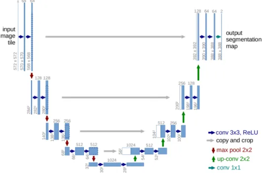
More recently, fully connected networks have been used for semantic segmentation (Long et al., 2015). This approach is based on the network architecture designed for image classification mentioned above and adds a layer to reproduce the size of the input image. Note that the image size no longer needs to be fixed: the output image has the same size as the input image. Based on this approach, the use of deconvolutions was then proposed (Noh et al., 2015). Unlike the previous network, this approach does not brutally reproduce the segmented image after several convolutions but allows to progressively enlarge the feature maps obtained to reproduce the image. This idea inspired Ronneberger et al. (2015) to propose a specific architecture for medical imaging: the U-Net (Figure 3.7). This architecture is now widely used and has been adapted for 3D medical image segmentation by C¸ i¸cek et al. (2016) and Milletari et al. (2016).

Figure 3.7 – U-net architecture, a fully convolutional network for medical image segmentation. (Ronneberger et al., 2015)

(44)

segmen-How to train a neural network? 35

tation (Chen et al., 2018) that introduces atrous convolutions (also called dilated convolutions). These convolutions introduce a new parameter called the dilation rate that defines a spacing between the input values considered. This allows a more global vision, supposed to be more adapted to segmen-tation than the convolutions used for image classification. The interesting results obtained by this approach show that, even today, image segmentation is a hot topic.

Although it is important to understand recent neural network architec-tures, automating image classification or segmentation does not only depend on the network organization. Training the network is also a critical step that I will discuss in the next section.

3.4 How to train a neural network?

The design evolution of the CNN architecture shows a tendency to create deeper models. However, the deeper the network, the more parameters it contains to learn and the harder the training is to converge. For a long time, training neural networks was almost impossible to converge in a reasonable time. The use of GPUs has considerably accelerated the process, especially as they become more and more powerful and accessible. However, today, it is mainly many tricks that help them to converge. In this section, I will briefly explain how a neural network is trained and then detail some of these tricks.

3.4.1 General approach

When a new data to be modeled is presented to the neural network, the first step is to calculate the output of the network: this is the forward propagation.

During training, we want to modify the architecture of the neural net-work, i. e. its parameters, so that the output obtained is closer to the desired one. For this purpose, a loss function is calculated. This function must be derivable and get higher values when the output is far from the expected learning value.

In order to minimize the loss function, several optimization algorithms have been proposed, the first and most common being the Stochastic Gra-dient Descent (SGD). SGD is a graGra-dient descent method used to minimize an objective function, here the loss function. The stochastic, i. e. random, side of this algorithm allows it to avoid small local minima and therefore to be more robust. When training a neural network, this algorithm adapts the parameters of each neuron by calculating the gradient of the loss function according to the parameter to be optimized. Depending on the gradient value, the parameter value is then adjusted to minimize the loss function.

(45)

In order to calculate the gradients for each parameter of the model, SGD uses backpropagation. This tool first calculates the gradients of the neu-ron parameters of the last layer, then iteratively goes up the network to calculate the gradients of the neuron parameters of the previous layers.

3.4.2 Tricks to improve training

In this section, I will discuss two of the main problems encountered when training a neural network: the vanishing/exploding gradient problem that prevents the network from learning and overfitting that makes the network learn incorrectly.

3.4.2.1 How to avoid the vanishing/exploding gradient problem? First of all, what is the vanishing gradient problem? During learning, gradi-ents are used to update neuron parameters. If these gradigradi-ents are too low, updating the parameters will have only a small impact. However, during backpropagation, the gradients of the model parameters with respect to the loss function are calculated by chain rule: each gradient is a multiplication of partial derivatives that depend on the previous layers. If some of these derivatives are close to zero, multiplying them will make the gradients even smaller, i.e. ” vanishing ”, which will cause the mentioned problem. This is all the more complicated to manage if the network is deep because the parameter gradients of the first layers will depend on an even higher number of partial derivatives. Conversely, if these gradients are greater than one, the gradient values may explode, causing the opposite problem: the parameters are unstable.

Now, how can we avoid it? First, by carefully initializing the parameters of the neural network. For example, Glorot and Bengio (2010) initializes the connection weights so that the input of the activation functions is nor-malized. Indeed, if the activation function is a sigmoid, input values too far from zeros have almost zero derivatives. Other activation functions have been proposed to avoid this problem: for example, the ReLU function has a zero derivative only for inputs below zero, large inputs will have the same derivative, i.e. one.

Then, the input data are generally normalized. Indeed, this makes it possible on the one hand to ensure that they are in the same range of values and on the other hand to avoid saturation of the activation functions. In the same vein, batch normalization aims to normalize the input of each layer during training.

3.4.2.2 How to deal with overfitting?

Another recurrent problem when training a neural network, especially when it is deep, is overfitting. This phenomenon is manifested by an increase

(46)

How to train a neural network? 37

of the neural network’s performance on the learning set, accompanied by a decrease on the validation set. In fact, neural networks are particularly data-intensive and easily overfit on small learning bases.

In order to limit overfitting, the first solution is to expand the size of the learning base. To do this, the data can be increased by various transforma-tions of the images: rotation, translation, cropping, noise effect, etc.

Another important step to avoid overfitting is the training design. In particular, the choice of the learning rate, the number of epochs, etc. For example, a too short learning time may lead to underfitting the model on the learning and test set, while a too long learning time may lead to overfitting on the learning set while having poor performance on the test set. In order to find the right balance, early stopping is generally used: this technique aims to stop learning when the model’s performance starts to deteriorate on a validation set, i.e. a part of the learning set reserved to test the model at each epoch.

Finally, one of the most popular tricks is the use of dropout during network training (Srivastava et al., 2014). This technique aims to ”drop out” some neurons during learning: a neuron is kept active according to a probability determined a priori, otherwise it is ”extinguished” (Figure 3.8). Thus, only a small network is trained on the data at this stage. The deleted neurons are then reintegrated into the network with their original weight.

Figure 3.8 – Illustration of the Dropout. (Srivastava et al., 2014)

Conclusion

To conclude, this chapter highlights the importance of choosing the archi-tecture of the neural network on the one hand and the training design on

(47)

the other. In this thesis, these CNN models inspired by the brain function will be tested to study one of its most striking anatomical characteristics: the cortical folds.

For the automatic classification of local folding patterns, a 3D ResNet will be used. Based on the study conducted by Hara et al. (2018) comparing the spatiotemporal 3D CNN adaptations of the 2D CNNs used for ILSVRC, a 3D ResNet has been choosen for the automatic classification of local folding patterns, as it is the architecture obtaining the best performance in (Hara et al., 2018).

For the automatic recognition of cortical sulci, two types of approaches will be tested: the first inspired by the patch segmentation approach pro-posed by Ciresan et al. (2012) and the second using a fully convolutional network, i.e. a 3D U-Net (C¸ i¸cek et al., 2016). These two approaches were initially proposed for the segmentation of medical images and have proven their effectiveness in this task.

(48)

Part II

(49)