HAL Id: hal-01399978
https://hal.inria.fr/hal-01399978
Submitted on 21 Nov 2016
HAL is a multi-disciplinary open access
archive for the deposit and dissemination of
sci-entific research documents, whether they are
pub-lished or not. The documents may come from
teaching and research institutions in France or
abroad, or from public or private research centers.
L’archive ouverte pluridisciplinaire HAL, est
destinée au dépôt et à la diffusion de documents
scientifiques de niveau recherche, publiés ou non,
émanant des établissements d’enseignement et de
recherche français ou étrangers, des laboratoires
publics ou privés.
MECSYCO: a Multi-agent DEVS Wrapping Platform
for the Co-simulation of Complex Systems
Benjamin Camus, Thomas Paris, Julien Vaubourg, Yannick Presse, Christine
Bourjot, Laurent Ciarletta, Vincent Chevrier
To cite this version:
Benjamin Camus, Thomas Paris, Julien Vaubourg, Yannick Presse, Christine Bourjot, et al..
MECSYCO: a Multi-agent DEVS Wrapping Platform for the Co-simulation of Complex Systems.
[Research Report] LORIA, UMR 7503, Université de Lorraine, CNRS, Vandoeuvre-lès-Nancy; Inria
Nancy - Grand Est (Villers-lès-Nancy, France). 2016. �hal-01399978�
MECSYCO: a Multi-agent DEVS Wrapping Platform for the
Co-simulation of Complex Systems
Benjamin Camus
1, Thomas Paris
1, Julien Vaubourg
2, Yannick Presse
2, Christine Bourjot
1, Laurent
Ciarletta
1, and Vincent Chevrier
11
Universit´e de Lorraine, CNRS, Inria, LORIA, UMR 7503, Vandœuvre-l`es-Nancy, F-54506, France.
[email protected]
2
Inria, 54600 Villers-l`es-Nancy, France. [email protected]
Abstract
Most modeling and simulation (M&S) questions about complex systems require to take simultaneously account of several points of view. Phenomena evolving at differ-ent scales and at differdiffer-ent levels of resolution have to be considered. Moreover, expert skills belonging to differ-ent scidiffer-entific fields are needed. The challenges are then to reconcile these heterogeneous points of view, and to inte-grate each domain tools (formalisms and simulation soft-ware) within the rigorous framework of the M&S process. To answer to this issue, we propose here the specifications of the MECSYCO co-simulation middleware. MECSYCO relies on the universality of the DEVS formalism in order to integrate models written in different formalism. This in-tegration is based on a wrapping strategy in order to make models implemented in different simulation software inter-operable. The middleware performs the co-simulation in a parallel, decentralized and distributable fashion thanks to its modular multi-agent architecture. We detail how MECSYCO perform hybrid co-simulations by integrating in a generic way already implemented continuous models thanks to the FMI standard, the DEV&DESS formalism and the QSS method. The DEVS wrapping of FMI that we pro-pose is not restricted to MECSYCO but can be performed in any DEVS-based platform. We show the modularity and the genericity of our approach through an iterative smart heat-ing system M&S. Compared to other works in the literature, our proposition is generic thanks to the strong foundation of DEVS and the unifying features of the FMI standard, while being fully specified from the concepts to their implemen-tations.
Keywords : DEVS, FMI/FMU, QSS, DEV&DESS, hy-brid modeling, parallel simulation, multi-agent
1
Introduction
In this article, we are interested in the modeling and simu-lation (M&S) of complex systems. These systems formed a particular type of dynamic systems defined as being ”com-prised of a great number of heterogeneous entities, among which local interactions create multiple levels of collective structure and organization”[1]. Complex systems can cor-respond to natural or artificial systems: the former range from insect colony (e.g. ants, bees, termites) to collective motion (e.g. crowds, birds flocking)[2], while the latter in-clude cities [3,4], traffic networks and smart grids.
By experimenting in a rigorous way on a simplification of a complex system (i.e. a model) instead of a real one, the M&S process avoids cost, time and ethic constraints, and thus position itself as a choice tool for the complex sys-tems science. However, when applied in this latter context, the M&S process faces many specific challenges. Indeed, most questions on complex systems require taking simulta-neously account of several points of view. Then, we need to consider phenomena evolving at different scales (temporal and spatial), and different levels of resolutions (from micro to macro). Moreover, the expert skills required for describ-ing a system may come from different domains (e.g. for a smart grid: the telecommunication, the information system, the electrical grid), each of them having their own tried and tested models and M&S tools (i.e. formalisms and simula-tion software). The challenges are then to reconcile these heterogeneous points of view, and to integrate each do-main models and tools within the rigorous framework of the M&S process.
A very promising strategy to tackles these challenges lies in co-simulation. Co-simulation consists in perform-ing a simulation by reusperform-ing models implemented in differ-ent simulation software, and managing exchanges of data between these software in order to make their models inter-act. It allows each specialist involved in a complex system
to keep using the tools which are popular in his/her com-munity while providing to each of them a realistic context. In addition, each simulator can (in some cases) execute on a different machine, which makes possible the co-simulation of very large systems. However, co-simulation faces many issues directly related to the heterogeneity of the models and tools that need to interact.
Our contribution to tackle these issues is twofold in this paper:
• We give the whole operational specification of the MECSYCO (Multi-Agent Environment for Complex-SYstem CO-simulation) co-simulation middleware dedicated to the DEVS (Discrete EVent System speci-fication) wrapping of pre-existing simulation tools. • We propose DEVS wrappers for the FMI (Functional
Mockup Interface) standard in order to make continu-ous equation-based models interact with discrete event models in a generic way.
The paper is organized as follows. Section2details the different challenges related to the M&S of complex sys-tems. Section 3 details how the DEVS formalism -and more precisely the DEVS wrapping strategy- offers an es-sential solution to these challenges. The Section4details the MECSYCO platform which enables the parallel simu-lation of complex systems models in a rigorous and decen-tralized way. Section5details the promising benefits of the FMI standard regarding the integration of equation-based tools, and how we achieve the DEVS wrapping of this stan-dard. Finally, in Section9we validate our proposition with a smart heating use case.
2
Co-simulation Challenges
2.1
Multi-representation integration
When modeling a non-complex dynamic system, we usu-ally describe the system at a specific level of resolution. However, in order to represent a complex system, several levels of resolution may be simultaneously considered (e.g. micro, meso, macro) [5]. Such multi-level representation could be needed, for instance, when there is a lack of ex-pressiveness of one level and a second one is required [6]; when available data explicitly refer to different levels of representation [5]; or when the modeling question is ex-plicitly to study the mutual influences between the cou-pled levels dynamics[7]. Finally, a multi-level represen-tation can be used in order to find a trade-off between a micro representation which offers more accurate results, and a macro representation which enables speeding-up the simulation[8,9,10].
As a consequence, the models involved in a co-simulation may have different representations of the sys-tem. The issue is then to reconcile the heterogeneous rep-resentations -i.e. given output data of a model which de-scribes the system at a level of resolution, what operations are needed to translate these data into the level of resolution of another model?
2.2
Multi-formalism integration
Because of its heterogeneity, a complex system may ex-hibit both discrete and continuous dynamics, and several formalisms maybe required to describe the system [11]. Such formalisms may be for instance differential or alge-braic equations for the continuous parts, and event-based, finite-state automata or one of the many formalization of the multi-agent paradigm for the discrete part.
As a consequence, discrete and continuous models may interact and co-evolve inside a co-simulation. At the ex-ecution level, this formalism heterogeneity implies deal-ing with different scheduldeal-ing policies: cyclic or variable time-steps, event-based, etc. A rigorous framework is then needed to integrate these different models in order to have an univocal behavior of the co-simulation [12].
Two solutions exist to integrate these different formalisms[11]:
Translate the models in a same formalism and per-form the simulation using the abstract simulator of this formalism. This is the solution chosen by AT oM3 [13], which enables to automatically translate two models by a sequence of transformations in their closest common for-malism. To do so, AT oM3relies on a Formalism Transfor-mation Graph where each node corresponds to a formalism and each arc represents an existing automatic translation. The shortcoming of this solution is that it forces to rewrite and re-implement the existing models, thus loosing the co-simulation advantages -i.e. effort of translation (if not auto-matic) and then possibilities of errors.
Use a hybrid M&S formalism which explicitly de-scribe how continuous and discrete systems interact and co-evolve. This super-formalism can be notably DEV&DESS [14] or HFSS (Heterogeneous Flow System Specification)[15], which merge a whole set of traditional techniques used in the field of hybrid modeling. Such tech-niques include notably (1) the integration of discrete in-put events during the evolution of the continuous system, and (2) the generation during the simulation of two kinds of discrete-events from the continuous system state: time-events and state-time-events[12]. While the former consist of events scheduled at predefined simulation times, the latter correspond to events whose occurrence is related to some specific condition on the continuous state (usually when a continuous variable cross a given threshold). From a
simu-lation perspective, the challenge is to integrate in a generic way this discrete-event logic during the numerical resolu-tion of the continuous system (this latter being concern with finding the best trade-off between the accuracy of the solu-tion and the simulasolu-tion performances[16]). Most notably, the detection and the accurate localization in time of state-events during the simulation is a well known issue in hybrid simulation [17].
2.3
Simulation software interoperability
From a software perspective, co-simulation implies deal-ing with a heterogeneous set of simulation software. In-deed, as shown in Table1, the different domain of expertise may have different simulation software which may be im-plemented in different programming languages and be com-pliant with different operating systems. Moreover some of these simulation software must be available only on some specific hardware (e.g. if a private license is required). In-teroperability processes are then required[18] to synchro-nize these heterogeneous software execution and manage exchanges of usable data between them [19].
This interoperability can be achieve in an ad-hoc way by directly modifying the simulation software to make them compliant with each others. A more generic solution con-sist of using a simulation middleware dedicated to the man-agement of the interoperability within the co-simulation. The advantage of this solution is its flexibility which en-ables easily adding, removing and changing some simula-tion software without impacting the rest of co-simulasimula-tion implementation. This is feasible because in this case, the simulation software do not have to be directly interoperable with each others, but have to be interoperable with the mid-dleware instead. The co-simulation midmid-dleware can also serves as a communication middleware thus enabling the distribution of the co-simulation, and being therefore com-pliant with the required hardware and OS diversity.
2.4
Synthesis
To sum up, setting up a co-simulation requires solving a set of specific issues at the representations, the formalisms and the software levels. The solutions that have to be provided are directly related to the heterogeneity found at each of these levels.
Additionally in a M&S process, the need for modular-ity is required -i.e. to enable adding, removing or changing models and simulation software and their connections with-out having to redefine all the co-simulation from scratch [24].
In order to fulfill this latter requirements, ad-hoc solu-tions should be avoided as a more generic and rigorous framework is needed. In the following we details how the DEVS formalism brings solution to these requirements.
3
DEVS as a pivotal formalism for
heterogeneity integration
3.1
The DEVS formalism
DEVS [25] is an event-based formalism for the M&S of system of systems. One important feature of DEVS is its universality which positions it as a pivot formalism for multi-paradigm modelling and simulation [26]. Indeed, not only DEVS appears to be universal for describing discrete-event systems [25], but it can also integrate continuous sys-tems [27] expressed for instance with differential equations [28]. Of particular interest in the scope of this article is the fact that, as shown by Zeigler[29], DEVS can also em-bed the DEV&DESS formalism [14]. This formalism offers a sound framework for describing hybrid systems as it de-scribes how continuous systems interact and co-evolve with the discrete world.
Moreover, DEVS can encapsulate differential and alge-braic equation solvers by relying on a quantized integrator approach like the Quantized State Systems (QSS) method [30]. This approach which is based on state quantization in-stead of the time discretization used by traditional integra-tion methods, shows in some case[31] better performance than these latter [32]. QSS is well-suited for hybrid mod-eling as it makes the continuous component equivalent to a DEVS model which naturally integrates input events, and makes state-events detection trivial and costless [33].
As summarized by Quesnel[28], the integration of a for-malism in DEVS can be performed either by a mapping or a wrapping. While the former consists in establishing the equivalence between the formalisms, the latter implies bridging the gap between the two abstract simulators [34]. The advantage of the wrapping strategy is to enable reusing pre-existing models already implemented in some simula-tion software [35].
DEVS distinguishes between atomic and coupled mod-els. A DEVS atomic model describes the behavior of the system and corresponds to the structure:
Mi= (Xi, Yi, S, δext, δint, λ, ta) (1)
where:
Xi= {(p, v)|p ∈ InP ortsi, v ∈ Xi} is the set of input
ports and values. These ports can receive external in-put events,
Yi= {(p, v)|p ∈ OutP ortsi, v ∈ Yi} is the set of output
ports and values. These ports can send external output events,
S is the set of the model states,
δext: Q × Xi→ S is the external transition function
Table 1: Example of M&S application domains and their simulation software.
Domain Simulation software Languages Operating system
Collective mo-tion
NetLogo [20] Java API Java & Scala GNU/Linux, Windows, Mac OS
GAMA [21] Java GNU/Linux, Windows, Mac OS
Telecom net-works
NS-3 [22] C++, Python API GNU/Linux
OMNeT++ [23] C++ GNU/Linux, Windows, Mac OS
Robotic VREP C/C++, Lua, Python, Java GNU/Linux, Windows, Mac OS
Physical system Dymola Proprietary code Windows
Matlab/Simulink Proprietary code, C/C++ API, Fortran GNU/Linux, Windows, Mac OS
Q = {(s, e)|s ∈ S, 0 ≤ e ≤ ta(s)} is the total state of the model,
e is the elapsed time since the last transition,
δint: S → S is the internal transition function describing
the internal dynamic of the model -i.e. the function processes an internal event which changes the model state,
λ : S → Yi is the output function describing the output
events of the model according to its current state, ta : S → R+0,∞ is the time advance function describing the
time during which the model will stay in the same cur-rent state (in the absence of input event). The function is used to get the date of the next internal event. A coupled model describes the structure of the system. It corresponds to the following structure which describes a set of interconnected atomic models:
N = (X, Y, D, {Md|d ∈ D}, EIC, EOC, IC) (2)
where:
X = {(p, v)|p ∈ InP orts, v ∈ X} is the set of input ports and values
Y = {(p, v)|p ∈ OutP orts, v ∈ Y } is the set of output ports and values,
D is the set of models id,
EIC = {((N, ipN), (d, ipd))|ipN ∈ InP orts, d ∈
D, ipd ∈ InP ortsd} is the set of external input
cou-plings,
EOC = {((d, opd), (N, opN))|opN ∈ OutP orts, d ∈
D, opd ∈ OutP ortsd} is the set of external output
couplings,
IC = {((a, opa), (b, ipb))|a, b ∈ D, opa ∈
OutP ortsa, ipb ∈ InP ortsb} is the set of
in-ternal couplings,
The closure under the coupling of DEVS is an important property which enables hierarchical modeling by proving that a coupled model is equivalent to an atomic one. Thus, a DEVS coupled model can be both composed of intercon-nected DEVS atomic and coupled models (these latter may be at their turn composed of coupled models etc.). DEVS proposes sequential and parallel abstract simulators and co-ordinators for respectively simulating the atomic and the coupled models. Thanks to the closure under the coupling of DEVS, these abstract simulators and coordinators can be controlled in an unified way using the DEVS simulation protocol.
3.2
Positioning
DEVS have striking advantages for managing the integra-tion of the formal and the software heterogeneity required by the co-simulation of complex system. This approach is the product of several decades of research, and constitutes a crucial scientific work we must capitalize.
In order to fulfill the requirements of complex system co-simulation, we propose to define a modular co-simulation middleware called MECSYCO (Multi-agent Environment for Complex SYstem CO-simulation) for managing in a generic way software interoperability. In this middleware, we propose to integrate heterogeneous formal models by using DEVS as a pivotal formalism in the following way:
1. integrate the different models in DEVS without imple-menting them again by using a wrapping strategy. 2. make these wrapped models interact within a DEVS
coupled model.
3. simulate the DEVS coupled model using the DEVS simulation protocol in order to perform the co-simulation in an unified way.
Thus, we respond both to the formal integration and to the software interoperability requirements of the complex system co-simulation (detailed in Section 2). In the fol-lowing section, we details the MECSYCO DEVS wrapping platform which is based on this proposition.
4
The MECSYCO platform
4.1
A Multi-agent Environment for M&S
MECSYCO [36] is a DEVS wrapping platform that takes advantage of the DEVS universality for enabling multi-paradigm co-simulation of complex systems. As shown in previous work [37], the platform also supports multi-level modeling. It is currently used for the M&S of smart electrical grids in the context of a partnership between LO-RIA/Inria1 and EDF R&D (leading French electric utility company) [38].
MECSYCO is based on the AA4MM (Agents & Arti-facts for Multi-Modeling) paradigm [39] (from an origi-nal idea of Bonneaud[40]) that sees an heterogeneous co-simulation as a multi-agent system. Within this scope, each couple model/simulator corresponds to an agent, and the data exchanges between the simulators correspond to the interactions between the agents. Thus, the co-simulation of the system corresponds to the dynamics of interaction between agents. Agents autonomy enables encapsulating legacy software by the use of wrappers[41]. Originality with regard to other multi-agent multi-model approaches is to consider the interactions in an indirect way thanks to the concept of passive computational entities called artifacts [42]. By following this multi-agent paradigm from the con-cepts to their implementation, MECSYCO ensures a mod-ular, extensible (i.e. features can be easily added such as an observation system) decentralized and distributable par-allel co-simulation. MECSYCO implements the AA4MM concepts according to DEVS simulation protocol for coor-dinating the executions of the simulators and managing in-teractions between models. In the following, we describe these concepts and their specifications.
4.2
MECSYCO Concepts
MECSYCO relies on four concepts to describe a co-simulation.
A model mi is a partial representation of the target
sys-tem implemented in a simulation software si (symbol in
Figure1a). A model possesses a set of input ports x1..n i and
output ports y1..m i .
An m-agent Ai(symbol in Figure1b) manages a model
mi and is in charge of the interactions of this model with
the other ones. Thus the m-agent is equivalent to a parallel abstract simulator for the models.
Each m-agent Ai sees its model mi as a DEVS atomic
model thanks to its model artifact Ii(symbol in Figure1d).
Therefore, Iiacts as a DEVS wrapper for mi- i.e. it
imple-ments the DEVS simulation protocol functions for control-ling mievolution through si.
1French IT research institute
(a) model (b) m-agent (c) coupling arti-fact
(d) model arti-fact
Figure 1: Symbols of the MECSYCO components.
Figure 2: Bloc diagram view of a DEVS coupled model.
Each interaction from an m-agent Ai to an m-agent Aj
is reified by a coupling artifact Ci
j (symbol in Figure1c).
A coupling artifact Ci
jworks like a mailbox: the artifact has
a buffer of events where the m-agents can post their exter-nal output events and get their exterexter-nal input events. Thus, a coupling artifact has two roles: for Ai, it is an output
coupling artifact, whereas for Aj it is an input coupling
artifact. The coupling artifacts can transform the data ex-changed between the models using operations that can be for instance, spatial and time scaling operations (convert-ing kilometers to meters or hours to minutes), or aggrega-tion/disaggregation operations [37].
According to the multi-agent paradigm, m-agents only have a local knowledge of the coupled model’s interconnec-tions. The coupled model’s internal coupling set IC is split such as an m-agent Ai only knows which input coupling
artifacts correspond to its model’s input ports, and which output coupling artifacts correspond to its model’s output ports. We define the set of input links INi of Aias being
composed of the couples (j, k) mapping the input coupling artifact Cij with the input port xk
i. We define the set of
out-put links OUTi of Ai as being composed of the couples
(n, j) mapping the output port yn
i with the output coupling
artifact Ci j.
The connection of the output ports of a model mi with
the input ports of a model mjis done by the coupling
arti-fact Cij. The link from a model mito a model mj(noted as
Li
j) corresponds to the tuple (n, k, o i,n
j,k). It maps the output
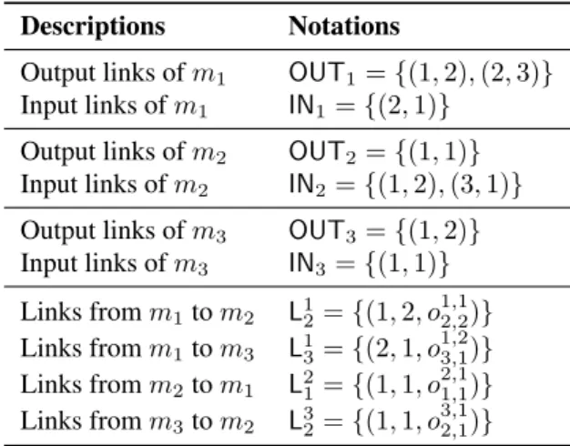
port yni with the input port xkj and applies the onk operation to transform the event between these two models represen-tation. By default, an operation corresponds to the identity operation id. The Table2and the Figure3illustrate how a DEVS coupled model (showed in Figure2) is described in a decentralized and distributable way thanks to MECSYCO.
Figure 3: Graphical representation of the MECSYCO co-simulation of Table2.
Table 2: Decentralized MECSYCO co-simulation of the DEVS coupled model of Figure2
Descriptions Notations
Output links of m1 OUT1= {(1, 2), (2, 3)}
Input links of m1 IN1= {(2, 1)}
Output links of m2 OUT2= {(1, 1)}
Input links of m2 IN2= {(1, 2), (3, 1)}
Output links of m3 OUT3= {(1, 2)}
Input links of m3 IN3= {(1, 1)} Links from m1to m2 L12= {(1, 2, o 1,1 2,2)} Links from m1to m3 L13= {(2, 1, o 1,2 3,1)} Links from m2to m1 L21= {(1, 1, o 2,1 1,1)} Links from m3to m2 L32= {(1, 1, o 3,1 2,1)}
4.3
Operational Specifications
The behavior of each m-agent corresponds to the DEVS conservative parallel abstract simulator which is based on the Chandy-Misra-Bryant (CMB) algorithm [43,44]. This algorithm is proven to be deadlock free and to respect the causality constraint [25] -i.e. to ensure that the ”execution of the simulation program on a parallel computer will pro-duce exactly the same results as an execution on a sequen-tial computer”[45].
Within this behavior, each m-agent Ai shares in its
en-vironment its Earliest Output Time estimate noted EOTi.
EOTicorresponds to the date (in simulation time), below
which Ai guarantees it will not send new external output
event. Aishares EOTiin the link time of each of its
out-put coupling artifact. The link time of a coupling artifact Cji is noted LTijand correspond to the simulated time (initially
equals to 0) up to which Aihas simulated the links from mi
to mj[43].
Each m-agent Ai uses the link times of all of its input
coupling artifacts to compute its Earliest Input Time esti-mate noted EITi. This EITicorresponds to the date (in
sim-ulated time) below which Aiwill not receive any new
ex-ternal input event. EITi corresponds to the minimum link
time of all of Ai’s input coupling artifacts.
For each m-agent Ai, all the events (internal or external)
with a timestamp inferior or equal to EITiare said to be safe
to process. In order to fulfill the causality constraint, each m-agent must process only safe events and in an increasing timestamped order.
Each EOTiis given by the Lookaheadifunction:
Lookaheadi() = min{nti, EITi+ Di, tini+Di} (3) with ntithe next internal event time of mi, tinithe time of the earliest event waiting to be processed in Ai’s input
coupling artifact, and Di(Di > 0) the minimum
propaga-tion delay of mi. This minimum propagation delay
cor-responds to the minimum delay (in simulated time) below which the processing of an external event can not schedule a new internal event in a model mi. Dihas to be determined
for each model miin the co-simulation.
This behavior which enables simulating a model until a time Z is formalized within the MECSYCO paradigm by the Algorithm 1 basing on the artifacts specifications de-tailed below.
A coupling artifact Cji proposes six functions to Aiand
Aj:
• post(en
out), n stores and transforms (according to
Ci
j’s operation) the external output event e k
outof output
port yin, in the artifact’s buffer.
• getEarliestEvent(k) returns the earliest exter-nal input event for the kthinput port of mj, xkj.
• getEarliestEventTime(k) returns the time of the earliest external event for xkj.
• removeEarliestEvent(k) removes from the ar-tifact’s buffer the earliest external event for xkj. • setLinkTime(ti)set LTijto ti.
• getLinkTime() returns LTij.
In order to manipulate mi, each model artifact Ii
pro-poses the following DEVS simulation protocol functions to Ai. These functions, which are listed below, have to be
de-fined for each simulation software:
• init() initializes the model mi. It sets the
parame-ters and the initial state of the model, • processExternalEvent(eini,ti,x
k
i)
pro-cesses the external input event eini at simulation time tiin the kthinput port of mi, xki,
• processInternalEvent(ti) processes the
in-ternal event of the model mischeduled at time ti,
• getOutputEvent(yn
i) returns e n
outi, the external output event at the nthoutput port of mi, yni,
• getNextInternalEventTime() returns the time of the earliest scheduled internal event of the model mi.
4.4
Implementation
MECSYCO is currently implemented in Java (available at
http://mecsyco.com) and C++. In order to make these two versions interoperable and to perform distributed co-simulations, MECSYCO relies on the JSON format and the OpenSplice implementation of the OMG standard DDS (Data Distribution Service). Using Opensplice, the cou-pling artifacts are divided in two parts, reader and writer, in order to split the co-simulation. DDS being based on the publish-subscribe communication pattern, writers coupling artifacts play the role of publishers while reader coupling artifacts act as subscribers. Each writer coupling artifact send data to its reader coupling artifact using a specific DDS topic (see Figure4).
The UML diagram of Figure 5 shows how we imple-ment the MECSYCO concepts following an object oriented programming. This implementation is in keeping with our multi-agent paradigm as each MECSYCO concept corre-sponds to a class of object, and as each autonomous m-agent corresponds to a thread. We retain then the advan-tages of our paradigm: the software architecture is com-posed of a set of modular software bricks which enables a decentralized and parallel simulation.
Figure 4: Distribution of a MECSYCO co-simulation.
4.5
DEVS wrapping of simulation software
So far, we successfully define DEVS wrappers for discrete modeling tools like the MAS simulator NetLogo [36], and the telecommunication network simulators NS-3 and OM-NeT++ [46]. Aside from several difficulties met when wrapping NS-3 and OMNeT++ (mainly due to the high level of modeling details offered by these platforms, as well as to the complexity of the opening and the distribu-tion of their telecommunicadistribu-tion models), making these dis-crete modeling tools compliant with the DEVS simulation protocol was a straightforward process. This is due to the fact that these platforms have a discrete modeling paradigm which is very close to DEVS.
However, to our experience with MECSYCO several dif-ficulties may arise when wrapping a simulation tools in DEVS. These problems depend mainly on two criteria:
• the M&S formalism used by the tools may not be explicitly defined by the software specification, and/or may be very different from DEVS. The challenge is then to answer the questions: what is the formalism used by the tools? How to bridge the formal gap be-tween this formalism and DEVS?
• the software interface with the middleware may be difficult to produce as the tools API and the software architecture are not always documented and fully com-pliant with the DEVS simulation protocol. Moreover, the software may not be conceived to be externally ma-nipulated.
Things getting especially complex with equation-based tools as their continuous modeling paradigm is very differ-ent from the discrete DEVS one. Thus, we need to bridge the gap between the discrete and the continuous paradigms, and a more complex wrapping strategy based on the hy-brid capacity of DEVS is required. Regarding this issue, wrapping each of these equation-based tools (e.g. Open-Modelica, Dymola, Matlab/Simulink) separately would be very inefficient.
Hopefully, a more efficient solution exists: most of these tools are compatible with the FMI standard which brings a generic API to manipulate equation-based models and
Algorithm 1 Aim-agent behavior. INPUT: INi, OUTi, Dti OUTPUT: nti← Ii.getNextEventTime() tini ← +∞ EOTi← 0 EITi← 0
. while the end of simulation. while (¬endOf Simulation) do
EITi← +∞
tini ← +∞
for all (j, k) ∈ INido
if Cij.getLinkTime()< EITithen . Compute EITi
EITi ← Cji.getLinkTime()
end if
if Cij.getEarliestEventTime(k) < tinithen . Take the next external event tini ← C j i.getEarliestEventTime(k) eini← C j i.getEarliestEvent(k)
p ← k . Save the corresponding input port
c ← j . Save the corresponding coupling artifact.
end if end for
. Compute EOTiand update output coupling artifact
if EOTi6= Lookaheadi(nti,EITi,tini)then EOTi← Lookaheadi(nti,EITi,tini) ∀(k, j) ∈ OUTi: Cij.setLinkTime(EOTi)
end if
. Find the next secured (internalor exteral) event if (nti ≤ tini) and (nti≤ EITi) and (nti≤ Z) then . if the event is internal
Ii.processInternalEvent(nti) . process the event
for all (k, j) ∈ OUTido . Send the resulting external output event
eoutk i ← Ii.getOutputEvent(yki) if eoutk i 6= ∅ then Ci j.post(eoutki, nti) end if end for nti← Ii.getNextInternalEventTime()
else if (tini < nti) and (tini ≤ EITi) and (tini≤ Z) then . if the event is external Ii.processExternalEvent(eini, tini, x
p
i) . process the event
Cc
i.removeEarliestEvent(p)
nti← Ii.getNextInternalEventTime()
end if end while
Figure 5: UML description of the MECSYCO software architecture.
their solvers. Our proposition is then to apply our DEVS wrapping strategy to FMI in order to define a generic way of making continuous equations-based tools inter-act with discrete-event one. In the following section, we detail the FMI standard and how we wrap it in DEVS using the hybrid M&S capacity of DEV&DESS and QSS.
5
DEVS wrapping of the FMI
stan-dard
5.1
The FMI standard
FMI [47] is a standard of the MODELISAR Consortium and the Modelica Association which proposes a generic software interface for manipulating equation-based models and their solvers. These models may be composed of a mix-ture of differential, algebraic and discrete-time equations, for instance described with the Modelica language. FMI aims at (1) defining a generic way of exchanging and using models designed with different equation-based simulation tools, and (2) protecting the intellectual property of these models by ensuring that they are seen as black-boxes.
A model implementing the FMI standard is called a Functional Mock-up Unit (FMU). The FMU interface dif-ferentiates the output variables whose values are accessi-ble from the outside (thus equivalent to the output ports of the model), from the input variables whose value can be set from the outside (thus equivalent to the input ports of the model). From a software perspective, this interface is composed of a set of C functions, and an XML file. The C functions enable controlling the FMU, whereas the XML file describes the FMU and its interface. More precisely, the XML file describes the variables names, types (i.e.
Real/In-teger/Boolean/String), variability (constant/discrete/contin-uous) and causality (input/output/parameter), as well as the continuous states vector.
So far around 42 simulation tools (e.g. Dymola, MAT-LAB/Simulink, OpenModelica) claim to be compliant with FMI v2.0 (80 with FMI v1.0), including 23 tools officially certified (29 with FMI v1.0)2. In order to support the stan-dard, these tools need either (1) to export their models as an FMU or (2) to import existing FMUs and use them as a component in a model. FMI allows two ways of exporting and importing a model: FMI for co-simulation and FMI for model-exchange.
With FMI for model-exchange, the model is exported without its solver. The FMU must be then associated with an external solver in order to be simulated. For that purpose, the solver can especially use the following C functions of the FMU API:
• fmi2GetReal/Integer/Boolean/String returns the current value of a given output variable. • fmi2SetReal/Integer/Boolean/String
sets a specific input variable to a given value.
• fmi2SetTime sets the clock of the model to a given simulated time.
• fmi2GetContinuousStates returns the contin-uous state vector.
• fmi2SetContinuousStates sets a the continu-ous state vector.
• fmi2GetDerivatives returns the derivative vec-tor of the continuous state.
2according tohttps://www.fmi-standard.org/tools
• fmi2CompletedIntegratorStep indicates that the integration step is finished, and evaluates if internal event has to be processed.
• fmi2GetEventIndicators returns indicators of state-events occurrence.
• fmi2EnterEventMode enters into the discrete event mode, i.e. makes the discrete-time equations ac-tive. While the FMU is in this mode, the integration of the continuous state is stopped but discrete-events (time, state or external) can be processed.
• fmi2EnterContinuousTimeMode enters into the continuous-time mode, i.e. disable the discrete-time equations. In this mode, the continuous state of the FMU can be solved, but the discrete state has to remain constant (i.e. events can not be processed). • fmi2NewDiscreteStates evaluates the
discrete-time equations (should therefore only be called in event mode) -i.e. processes the potential time and state events. Information returned by this function includes (1) the date of the next time-event (if scheduled), (2) indication if the processed event(s) has changed the continuous state (thus creating a discontinuities in the state trajectory), and (3) indication if the discrete state has to be immediately re-evaluate (e.g. to solve an in-ternal algebraic loop).
With FMI for co-simulation, a model is exported with its solver. As this solver has a passive behavior, an FMU for co-simulation is considered as a slave, and proposes in par-ticular the following C functions in order to be controlled by a master algorithm[48]:
• fmi2DoStep performs an integration for a given du-ration.
• fmi2SetReal/Integer/Boolean/String set a specific input variable to a given value. • fmi2GetReal/Integer/Boolean/String
get the current value of a given output variable. • fmi2GetFMUState and fmi2SetFMUState are
optional (but essential[49]) functions used to to ex-port/import the model state. They enable therefore to perform a rollback during the simulation of the model. FMI gives generic guidelines on how a master must man-age a set of interconnected FMUs in order to jointly solve their equations: the FMUs executions are synchronized thanks to communication points. These communication points which are shared by all the FMUs, correspond to the points in the simulated time where (1) the FMU simulation
must be stopped, and (2) exchanges of data has to be per-formed between FMUs according to their output-to-input links.
Aside from these guidelines, FMI does not give the specification of the master algorithm. As a conse-quence, different master algorithms are currently developed like FIDE[50] (FMI Integrated Design Environment) and DACCOSIM[51] (Distributed Architecture for Controlled CO-SIMulation), and numerous issues related to the dis-tributed numerical resolution of the system[49] are still un-der investigation by the community (e.g. how to determine the best communication points interval during the simula-tion? how to manage algebraic loop between FMUs?).
Rather than focusing on these distributed numerical reso-lutions aspects which arise when several FMUs are directly interconnected, we focus in this paper on the hybrid sim-ulation issues which arise when an FMU interact with a discrete-event component (e.g. a NS-3 model). Indeed, in a hybrid context, the communication points simulation strat-egy of FMI faces the following issues:
• state events occurring between 2 points of communi-cation are localized at the upper communicommuni-cation point, pending improvements of the hybrid co-simulation in the FMI standard.
• new inputs are only taken into account at the next com-munication point no matter when they are received (the abort orders are only applied at the communication points).
An effort is thus required to integrate the operational soft-ware in such a way as to respond to events. For that purpose, we present in the following our DEVS wrapping strategy for FMU. As FMUs for co-simulation and FMUs for model exchange do not have the same API and do not convey the same constraints, we specify a different wrapper for each of them in order to be fully compliant with the standard.
5.2
Wrapping strategies
As any model in MECSYCO, an FMU to integrate will be connected to the co-simulation by a model artifact. This ar-tifact exposes a DEVS view of the FMU, and must allow it to deal with events. To define such a model artifact we can rely on the DEV&DESS formalism as it can be embedded into DEVS, and as it offers a sound framework for describ-ing hybrid systems.
As defined by Zeigler [29], the DEVS version of a DEV&DESS model is composed of three components, each of them being formalized as a DEVS atomic model. With this structure, a DEV&DESS model can be incorporated into a larger DEVS schema as a coupled model. Thus the DEV&DESS model can be simulated using the DEVS
simulation protocol. The three components composing the model are:
• A continuous component describing the evolution of the continuous part of the system according to contin-uous inputs, and producing contincontin-uous outputs. • An event-detection function determining when
state-events occur based on the continuous states of the model (i.e. the FMU state in our case).
• A discrete-event component describing the evolution of the discrete part of the system. This component de-scribes the behavior of the model in the discrete-world, that is to say how it schedules internal events, how it produces and reacts to discrete inputs (i.e. exter-nal events), and what are the impacts of state-events. Potentially, for each of these events, the event-based component can change the whole DEV&DESS states, that is to say (1) its own state, (2) the continuous com-ponent state (thus creating a discontinuity in the state trajectory) and (3) the event detection function. The two strategies we propose to wrap FMUs in DEVS using DEV&DESS are the following:
• FMI for model-exchange proposes primitives that can handle an hybrid model. However, as stated in Section 5.1, in order to be simulated an FMU for model-exchange needs to be associated with a solver. We need then to implement such an hybrid solver in our DEV&DESS wrapper. In order to manage the continuous state simulation, the original DEVS ver-sion of DEV&DESS relies on a quantized integrator approach. The rationale behind this choice is that, quantized integrators have a discrete-event behavior as they quantize the states space instead of discretizing the time dimension. Thus, a quantized integrator nat-urally bridge the gap between the continuous and the discrete-event worlds [33]: its working principle is al-ready based on the integration of inputs events and on the detection of state-events[30] (i.e. localizing when the state trajectory cross a given threshold). It makes then perfectly sense to keep this choice and to imple-ment a quantized integrator in our wrapper. More pre-cisely, we choose the QSS approach[30] (developed mainly by Kofman) as it offers some of the most ad-vanced mathematical solutions for solving equation-based system, while exhibiting striking simulation per-formances. We have currently implemented QSS1 [52] (i.e. first order numerical method) and QSS2 [32] (i.e. second order numerical method) solvers for FMU. • FMI for co-simulation embeds a solver but does not
include yet the primitives required for managing a discrete-event behavior[53,49,50] (e.g. the date of
the next scheduled time-event can not be obtained from the FMU). Therefore, we consider that FMI for co-simulation only specifies the continuous behavior of the system. We need then to specifies its dis-crete behavior (i.e. the equivalent of the DEV&DESS event-detection function and the discrete-event com-ponent) within our wrapper. Additionally, specifying the discrete-event behavior outside the FMU enables a more flexible wrapping: different discrete-event be-haviors can be associated with a single FMU depend-ing on the co-simulation context (e.g. the discrete-event component can produce a discrete output sig-nal by regularly sampling the continuous output of an FMU, or send events when the continuous output signal of the same FMU reaches a given threshold). Moreover, when wrapping an FMU for co-simulation in DEVS, we have to take account of an additional constraint: the FMU is exported with its time-stepped solver as a black box onto which we have a limited control. By its time-stepped nature, an FMU can not be considered as a QSS model, and therefore we need to adapt the original DEVS version of DEV&DESS in our model artifact.
The two next sections detail our wrappers and their vali-dations.
6
Wrapping of FMU for
model-exchange
Figure 6a shows the architecture of our QSS2 solver for FMU. This architecture follows mainly the one defined by Kofman, but also has slight differences because two crite-ria where not handled by the original QSS specifications: (1) due to the FMU nature, the model is clearly separated from its solver, and (2) the discrete-events may cause dis-continuities in the continuous state trajectory. In order to highlight these differences, we now describe how our QSS solver works (Section 6.1) and how it interacts with the other components of DEV&DESS: the state-event detec-tor (Section 6.2) and the discrete-event behavior compo-nent (Section6.3). This whole structure of the wrapper is detailed in Figure6band corresponds to a DEVS coupled model which is managed by a classic DEVS coordinator not detailed here for sake of concision. This coordinator is directly controlled by the API of the MECSYCO wrapper. Section6.4details the validation of the wrapper.
6.1
Continuous behavior simulation with
QSS
In the original QSS specifications, the solver interacts with two clearly separated function blocks which respectively
(a) QSS2 solver for FMU model-exchange (b) global view
Figure 6: bloc diagram view of the DEVS wrapper for FMU model-exchange
define the output and the input behaviors of the model. In our wrapper, these blocks are directly embedded inside the FMU. Therefore the outputs (both discrete and continuous) of the solver correspond to the FMU ones. The output ports of our wrapper coupled model are directly linked to the FMU ones. However, according to the standard, the FMU discrete output ports produce piecewise-continuous signals -i.e. these signals are always present no matter the time instant[50]. In order to generate discrete-event output sig-nals (i.e. sigsig-nals that are present only at some instants in time) for these discrete ports, we propose an optional mode in our wrapper which filters the output of the FMU in order to generate signals (i.e. external events) only at the mo-ments of the time and/or state-events.
In accordance with the QSS approach, each variable xiof
the FMU continuous state vector is associated with a DEVS quantized integratorR
i. Each integrator
R
itakes in input the
first and second derivatives of xirespectively noted uiand
mui, and produces in output the new values and slopes of
xinoted respectively qiand mqi. These integrators
numer-ically solve the equation in an asynchronous way. A DEVS atomic model f is in charge of computing the derivatives slopes, handling the inputs of the equationbased system -therefore the model has a set {in1..inm} of input ports
cor-responding to the FMU ones- and interacting with the in-tegrators. In the original QSS specifications, the equation-based system is directly embedded into f . This is not feasi-ble in our case cause the system is already embedded in an
FMU. As a consequence, in our solver f also manages the interaction with the FMU in the following way:
• when it has to update the FMU continuous state (e.g. when it receives from an integrator a new value and slope for a continuous state variable), f first switches the FMU into the continuous mode (using fmi2EnterContinuousTimeMode) if it was not already, and call the fmi2SetContinuousStatesfunction.
• when it has to update the value of an input variable of the FMU (i.e. when it receives an input event through a ini ports), f first checks the variability
of the variable into the XML description file. De-pending if this variability is continuous or discrete, f calls the fmi2EnterContinuousTimeMode or fmi2EnterEventMode function in order to set the FMU in the appropriate mode (if it was not already). f checks then the input variable type in the XML file, and updates its value in the FMU using fmi2SetReal/Integer/Boolean/String function. If the updated variable is discrete, f asks (several times if needed by the FMU) the FMU to re-evaluate its discrete state using fmi2NewDiscreteStates.
• when it receives any events at its input ports (e.g. from the integrators or at a ini port), f updates the clock
of the FMU to the timestamp of the events using the fmi2SetTimefunction.
• when it has to get the derivative ui (e.g. in order to
compute its slope muiand to forward these two values
toR
i), f uses the fmi2GetDerivatives function
of the FMU.
As shown in Figure 6b the solver interacts with two atomic models in order to simulate the discrete behavior of the FMU. These models correspond to the ones defined by Zeigler in the DEVS version of DEV&DESS.
6.2
State-event detector
The state-event detector atomic model is in charge of the accurate localization of state-events during the simulation of the continuous equations. In order to take advantages of the QSS approach for detecting state-events, we make the hypothesis that the state-event thresholds of the FMU are a prioriknown (either because this information can be ob-tained from the model designer or from the XML descrip-tion file). In the original hybrid QSS specificadescrip-tions[33], Kofman suggests two ways of feeding the state-event de-tector from the QSS solver:
1. It can receive the variables values q and derivatives u and mu. This way, as stated by Kofman, the detector only ”have to find the roots of a second degree poly-nomial”[33] in order to find the time of the next state-event (in the absence of new state and derivatives up-date received from the solver). The detector schedules then an internal event at the time of this state-event in order to produce an output notifying the occurrence of the event.
2. Or it can only receive the derivatives u and their slopes mu directly from the output ports of f . In this case, in addition to find the time of the next state-event and schedule the resulting internal event, the detector has to integrate (in parallel of the system resolution) the variables concerned with the thresholds.
Kofman opts for the second option as it does not implies any modification of the QSS solver. However, the drawback of this option is that the detector can not be aware of the discontinuities in the continuous state trajectory caused by discrete-events processing (time, state or external). That is why we choose the first option in our wrapper: the model f forward immediately to the detector all the updates of the continuous states vector q and its derivatives u and mu through a dedicated output port.
6.3
Discrete-event behavior simulator
The DEVS’ atomic model is in charge of managing the oc-currences of discrete events (state, time and external). After
each modification of the discrete state of the FMU -i.e. after each external/time/state-event processing in the FMU-, this component (1) retrieves the time tn of the next time-event scheduled in the FMU, and (2) checks if the event process-ing has created a discontinuity in the continuous state trajec-tory (by checking the information returned by the last called of the FMU fmi2NewDiscreteStates function). The DEVS’ component schedules an internal event at each tn. It also receives notifications of state-events occurrences from the detector. Moreover, all the discrete inputs of the FMU are first sent to the DEVS’ component before being immedi-ately forwarded to the QSS solver. This enables the DEVS’ component to be aware of discrete-input occurrences, and thus to interact with the FMU (i.e. update tn and check dis-continuities) after the discrete input was processed by the solver. Therefore as shown in Figure6b, we distinguish in the QSS solver interface between:
• the set {inc
1, ..., inck} of input ports which correspond
to the continuous inputs of the FMU. These ports are directly connected to the input ports of the wrapper. This way, the solver can directly receive continuous inputs of the FMU from the other simulation tools of the co-simulation.
• the set {ind
1, ..., indl} of input ports which correspond
to the discrete inputs of the FMU. These ports are du-plicated in the DEVS’ component interface.
As soon as it computes a time event or it receives a state-event notification, the DEVS’ component sends an inter-nal event notification to the QSS solver through a dedicated port. The solver processes this notification in the same way it does with discrete inputs: it sets the FMU to the discrete mode and asks the FMU to re-evaluate its discrete state, thus causing the time/state-event to be processed. The only difference is that, as no discrete input of the FMU corre-sponds to this internal event notification port, the solver does not change any input variable of the FMU. Finally, as soon as the DEVS’ component detects a discontinuity in the continuous state trajectory, it sends immediately a reset event to the QSS solver through a dedicated port. In accor-dance with Zeigler’s DEV&DESS specifications, this event resets both the quantized integrators and the f model state, thus enabling the QSS solver to handle the discontinuity.
6.4
Implementation and validation
We have implemented this wrapper in the Java version of MECSYCO. In order to interact with the FMU, we rely on JavaFMI[54]. As this library only covers FMU for co-simulation, we proposed an extension to interact with FMU for model-exchange. We have verified the behavior of our wrapper by reproducing two QSS2 use-cases proposed by
Kofman[33]. The first one corresponds to an DC-AC in-verter circuit equipped with switches controlled by discrete-inputs which are sent according to a Pulse Width Modula-tion (PWM) strategy. The second one corresponds to a ball bouncing downstairs with state-events occurring twice each bounce (one when the ball hits the ground and one when it leaves it). We translated the Kofman’s models into the Modelica language (Figures7aand8a) and export them in FMUs for model-exchange using OpenModelica. We found similar simulation results (Figures7band8b) and perfor-mances with our solver and with the Kofman one.
As these two models do not include discontinuities in the continuous state trajectory, we also propose another use case to test this aspect with our solver (Figure9a). This use case correspond to the simulation of a a barrel-filler factory inspired by the one proposed by Praehofer[14]. In this fac-tory, we consider a queue of barrels waiting on a conveyor to be filled. The factory fills only one barrel at a time. As soon as the water reaches a given level in the barrel, the barrel is carried away by the conveyor, and the filling pro-cess starts again for the next empty barrel. A tank stores the water to fill the barrels. The flow rate of water filling the barrel decreases with the level of water in the tank. A valve controls the flow of water between the tank and the barrel. The valve can only be in two states ”open” (water goes from the tank to the barrel) or ”close” (the filling pro-cess is stopped). The continuous dynamics of the model correspond to the levels of water in the current barrel and in the tank. The model receives discrete inputs controlling the valve. State-events correspond to the moment where the current barrel is full. At this point, the level of water in the current barrel is reset to represent the change of barrel. The model produces a discrete output signal corresponding to a regular sampling of the level of water in the barrel. This signal can be for instance sent to a controller for monitoring the filling process. We found similar results when simulat-ing this model with our QSS2 solver (Figure9b) and with the OpenModelica solvers.
7
Wrapping
of
FMU
for
co-simulation
As stated in Section 5.2, we need the three components of DEV&DESS to integrate a FMU into DEVS. An FMU for co-simulation provides the continuous behavior and we need to define the two remaining components (i.e. the state-events detector and the discrete-behavior component) in the wrapper. These components are dependent of the wrapping context:
• the discrete-behavior component has to specify the be-havior of the FMU in the discrete world. This com-ponent corresponds to a DEVS atomic model which
can interact with the FMU component. For example, this component can sample a continuous output of the FMU by regularly scheduling internal event, and pro-ducing external output event according to the current value of the FMU variable using fmi2GetReal. • the state-events detector has to specify the condition of
occurrence of state-events according to the FMU state. This detector corresponds to a boolean function S → {true, f alse} with S the set of the FMU states. For example, this function can return true (i.e. a state-event occurs) only if a variable of the FMU is superior or equals to a given value.
In the following we detail how we implement the main DEVS primitives into the wrapper.
7.1
Time of the next internal event
In our DEVS wrapper for FMU for co-simulation[55], we rely on the FMI specifications to simulate the continuous output of the component: we consider that the FMU pro-duces outputs at a sequence of pre-defined communication points. From our DEVS point of view, these communica-tion points are seen as internal events producing external output events. In the same way, from our DEVS point of view we see updates of the continuous input values received by the FMU as input events.
According to the DEVS semantic, the getNextInternalEventTime() function must return the date of the earliest scheduled internal event in the model. In the DEV&DESS context, this date corresponds to the minimum between:
• the date of the next internal event scheduled in the discrete-event component,
• the date of the next communication point of the FMU, • the date of the next state-event.
Getting the first two dates is trivial as they are a priori known. Things get more complex for the state-events: be-cause of the numerical resolution of the equational model, state-events can only be detected after each integration step of the FMU, and their localization in time can only be ap-proximated.
In order to get the date of the next state-event, we need to perform an exploration with the FMU to see if a state-event will occur before its next communication point. Thus, the component will always be ”in the future” compared to the current simulation time. As according to the DEVS se-mantic the getNextInternalEventTime() function must not change the state of the model, it is imperative to be able to come back to the previous state of the FMU which is the only legitimate state from the simulation point of view.
model BouncingBall
output Real x(start = 0.575); "horizontal position (m)" output Real y(start = 10.5); "vertical position (m)" output Real vx (start = 0.5); "horizontal speed (m/s)" output Real vy(start = 0); "vertical speed (m/s)" discrete Integer sw(start=0); "discrete position" parameter Real k = 100000;
parameter Real m = 1; parameter Real b = 30; parameter Real ba = 0.1;
parameter Real g = 9.80665; "gravity (m/sˆ2)" parameter Real h = 10; "first step height (m)" equation
der(x) = vx; der(y) = vy;
der(vy)=-g-ba*vy/m-sw*(b*vy/m+k/m*(y-floor(h+1-x))); der(vx)=-ba/m*vx;
when y<=floor(h+1-x) and pre(sw)==0 then sw= 1;
elsewhen y>=floor(h+1-x) then sw= 0;
end when; end BouncingBall;
(a) Modelica code of the model (b) MECSYCO simulation results
Figure 7: Simulation of the bouncing ball system
model inverter-circuit
parameter Real R = 0.6 "resistance (ohm)"; parameter Real L = 0.1 "inductance (H)"; parameter Real Vin = 300; "input voltage (V)" Real iL(start = 0) "current (A)";
discrete input Integer sw(start = -1) "switch"; equation
der(iL) = (-R / L) * iL + sw * Vin; end inverter-circuit;
(a) Modelica code of the model (b) MECSYCO simulation results
Figure 8: Simulation of the DC-AC inverter circuit
model barrel
discrete input Boolean valve(start = true); parameter Real qmax = 7 "initial tank water (L)"; Real q(start = qmax) "water in the tank (L)"; Real flow(start = 0) "flow of water"; parameter Real gain = 0.3;
parameter Real value = 0.025;
output Real x(start = 0) "water in the barrel"; parameter Real xmax = 1 "wanted barrel water(L)"; parameter Real f = 10 "sampling frequency";
discrete output Real y(start = 0) "output sampling"; equation
flow = if valve and q > 0 then q*gain+value else 0; der(q) = -flow;
der(x) = flow; when x >= xmax then
reinit(x, 0); end when;
when sample(0, 1 / f) then y = x;
end when; end barrel;
(a) Modelica code of the model (b) MECSYCO simulation results
The rollback capability of the FMU assures this feature as long as no new integration step is performed.
When a state event is detected during an exploration, we perform a bisectional search [17,56] in order to localize the state-event as precisely as possible in the time. This search is formalized by the Algorithm 2 which, given the initial integration step ∆T and a number of iterations m (formal-izing the search precision), positions the FMU as close as possible to the state-event occurrence. The algorithm basi-cally progresses by a succession of integration steps whose duration δt is adapted according to state-event occurrences, and following a dichotomous strategy. As, again, the orig-inal state must always be accessible, and as only one inte-gration step can be canceled at a time, the algorithm always goes back to the legitimate state before performing a new integration step.
Algorithm 2 Bisectional search for state-event localization. INPUT: ∆T ∈ R+0, m ∈ N + 0 δt ← 0 ∆t ← ∆T for 1 to m do fmu.rollBack() ∆t ← ∆t/2 fmu.doStep(δt + ∆t) if ¬stateEventOccurence() then δt ← δt + ∆t end if end for
7.2
Events processing
According to the DEV&DESS semantics, when an event (internal, external or state-event) occurs at simulated time t, the equational component describes the continuous evo-lution of the system until t, and the event is processed by the discrete-event component. This behavior is translated in our model artifact as follows.
When the processExternalEvent(eini,t,x
k i)
function is called to report the occurrence of an external input event einiinto the x
k
i input port, the first step consists
in rolling back the FMU to its previous state, which is, as stated in the previous section, the only legitimate state from the simulation point of view. Then the FMU performs an integration step until t in order to reach the point where the event occurs. Finally, if xki is a continuous port, the FMU is parametrized accordingly. If xki is a discrete port, the
ex-ternal transition function of the discrete-event component is triggered in order to process eini.
In a similar way, when the
processInternalEvent(t) function is called to process the next internal event, the FMU is rolled back to
its previous state and an integration step is performed until t. If the next internal event corresponds to a communication point of the FMU, then the model artifact retrieves the continuous output ports values, and produces the external output events accordingly. On the other hand, if the next internal event corresponds to a state-event or the next internal event of the discrete-event component, then the internal transition function of this latter is called, which could produce external output events.
8
Discussion and related works
We have presented in Section4the whole specification of the MECSYCO middleware which enables the rigorous co-simulation of complex systems. On the contrary to the mo-saik co-simulation platforms [57] which is based on discrete time-step framework, MECSYCO enables the rigorous in-tegration of models written in heterogeneous formalisms. Indeed, on this point MECSYCO relies on the formal guar-antees offered by DEVS, and on the practical guidelines of-fered by the numerous integrative works around DEVS in the literature.
The High Level Architecture (HLA) standard [58] gives generic guidelines and rules for building a co-simulation middleware. It as been shown that an HLA-compliant mid-dleware, can also used a DEVS framework [59,60]. How-ever, on the contrary to HLA, we gives here the whole specification of our platform. These specifications range from the decentralized synchronization algorithm to the distributed agent-based architecture and its object oriented implementation. Thus, we clearly define our middleware working principle, making our co-simulations more repro-ducible and our middleware more flexible: different imple-mentations of MECSYCO are interoperable and therefore can be simultaneously used in a co-simulation, as shown with our Java and C++ versions.
Finally on the contrary of the DACCOSIM [51] plat-form dedicated to the co-simulation of FMU components, MECSYCO is not limited to a specific simulation software or norm.
Using our MECSYCO platform, we have shown how FMU components can be wrapped into a DEVS model us-ing DEV&DESS and QSS. We propose then a generic way of making continuous models exported in the FMI standard interacting with discrete models. It is important to note that, as we base this wrapping directly on the DEVS protocol, this work is not limited to the MECSYCO platform, but can be implemented in any DEVS-based platform. With our DEVS wrapping of FMU for model-exchange, we define a hybrid QSS solver tailored to the FMI standard. Like other existing QSS versions of the litterature [61,62], our solver can simulate Modelica models. However, the originality is that our QSS solver can also solves models written in any
of the numerous software compliant with FMI for model-exchange (e.g. MATLAB/Simulink).
We also want to underline the fact that, whereas our wrapping of FMU for model exchange is adapted both for FMI 1.0 and 2.0 versions, our wrapping of FMU for co-simulation is only adapted for FMI 2.0. This is due to the fact that we rely on the roll-back capacity of the FMU which is only available in the latest version of the standard.
In the following section, we show the features of our so-lutions through a proof of concept of a smart heating M&S.
9
Use Case
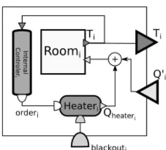
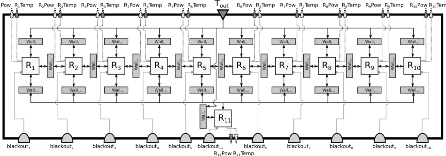
Our use case is inspired by different works around smart-heating [62][63]. We want to simulate the evolution of the temperature inside a system composed of two buildings equipped with electric heaters, and the power consumption of these latter. Using this simulation, we are interesting in the design of a controller for limiting the consumption peaks duration in the building. To do so, this controller temporarily disables some heaters according to the infor-mation it receives on the buildings temperatures and power consumption. This controller interacts with the buildings system through an IP telecommunication network. Such a goal could lead to an typical iterative M&S process driven by the following series of questions:
1. What are the power consumption and the temperatures evolution in the buildings without the controller? 2. Does the controller actually achieve its goal without
the delays and the interference induced by the telecom-munication network?
3. What are the influences of the telecommunication net-work on the controller performances?
This leads to three major steps in the M&S process. In order to answer to the first question, we need to sim-ulate the thermic system. We use three models. One scribes the outside temperature evolution. One model de-scribes the power consumption and temperature evolution of one building according to the outside temperature evo-lution. We perform the co-simulation of these three models by feeding the building models with the outside temperature trajectory.
In order to answer the second question, we build the model of the controller. We use this model twice (one for each building) in the co-simulation. Each controller model is fed with the outputs of its building model (i.e. rooms temperatures and power consumption). When needed, it produces as output the heaters switch off/on orders which are sent to the building models as inputs.
In order to answer the last question, we add a model of the telecommunication network between the buildings and
their controller. The outputs of the buildings models now first pass through the network model before arriving to the controller models. Reciprocally, the controller orders tran-sit through the network model before delivery. The network model adds then delays and perturbation (i.e. packet loss and noise) to the system.
This ”toy” use case does not claim to be realistic. We keep the individual models of the use case simple since we are here more focused on demonstrating the following MECSYCO properties rather than on presenting a credible use case:
• Modularity: the use case development follows an it-erative M&S process. We first begin the co-simulation with the thermic model of the building. Then, we add step by step the models of the controller and the telecommunication network. We show that passing from one of these steps to another does not require to rebuild the co-simulation from scratch.
• Software interoperability management: each model of the co-simulation is implemented in a different simulation software. The thermic model is defined in Modelica and exported into FMUs for model-exchange and co-simulation, the telecommunication model is defined using the NS-3 simulator, and the controller model is implemented in an ad-hoc way us-ing the Java language. We show that MECSYCO prop-erly manages the exchange of data between these het-erogeneous software.
• Multi-formalism integration: the models of the co-simulation are defined in different formalisms. The thermic model is an hybrid model composed of differ-ential and discrete equations. The telecommunication model is a discrete event model whereas the controller model is a discrete time-stepped model. We show that MECSYCO enables the rigorous integration of these heterogeneous models.
• Multi-representation integration: the models evolve at different temporal scales, namely the seconds for the controller and the thermic models and the nanosec-onds for the telecommunication network. We show that MECSYCO rigorously synchronizes these mod-els executions during the co-simulation.
• Distributed multi-platform execution: we execute the co-simulation on two computers connected on a LAN. These two computers uses different op-erating systems, and different implementations of MECSYCO. The telecommunication network model is executed on GNU/Linux Debian with the C++ ver-sion of MECSYCO, whereas the other models are exe-cuted on Microsoft Windows 10 with the Java version of MECSYCO.