HAL Id: hal-02586024
https://hal.sorbonne-universite.fr/hal-02586024
Submitted on 15 May 2020
HAL is a multi-disciplinary open access
archive for the deposit and dissemination of
sci-entific research documents, whether they are
pub-lished or not. The documents may come from
teaching and research institutions in France or
abroad, or from public or private research centers.
L’archive ouverte pluridisciplinaire HAL, est
destinée au dépôt et à la diffusion de documents
scientifiques de niveau recherche, publiés ou non,
émanant des établissements d’enseignement et de
recherche français ou étrangers, des laboratoires
publics ou privés.
Nils Haëntjens, Alice Della Penna, Nathan Briggs, Lee Karp-Boss, Peter
Gaube, Hervé Claustre, Emmanuel Boss
To cite this version:
Nils Haëntjens, Alice Della Penna, Nathan Briggs, Lee Karp-Boss, Peter Gaube, et al.. Detecting
Mesopelagic Organisms Using Biogeochemical-Argo Floats. Geophysical Research Letters, American
Geophysical Union, 2020, 47 (6), pp.e2019GL086088. �10.1029/2019GL086088�. �hal-02586024�
Detecting Mesopelagic Organisms Using
Biogeochemical-Argo Floats
Nils Haëntjens1 , Alice Della Penna2,3 , Nathan Briggs4 , Lee Karp-Boss1 , Peter Gaube2 , Hervé Claustre5 , and Emmanuel Boss1
1School of Marine Sciences, University of Maine, Orono, ME, USA,2Applied Physics Laboratory, University of
Washington, Seattle, WA, USA,3Laboratoire des Sciences de l'Environnement Marin (LEMAR), UMR 6539,
CNRS-Ifremer-IRD-UBO-Institut Universitaire Européen de la Mer (IUEM), Plouzané, France,4National
Oceanography Centre, Southampton, UK,5Laboratoire d'Océanographie de Villefranche, UMR 7093, CNRS et
Sorbonne Université, Villefranche-sur-mer, France
Abstract
During the North Atlantic Aerosols and Marine Ecosystems Study in the western North Atlantic, float-based profiles of fluorescent dissolved organic matter and backscattering exhibited distinct spike layers at ∼300 m. The locations of the spikes were at depths similar or shallower to where a ship-based scientific echo sounder identified layers of acoustic backscatter, an Underwater Vision Profiler detected elevated concentration of zooplankton, and mesopelagic fish were sampled by a mesopelagic net tow. The collocation of spike layers in bio-optical properties with mesopelagic organisms suggests that some can be detected with float-based bio-optical sensors. This opens the door to the investigation of such aggregations/layers in observations collected by the global biogeochemical-Argo array allowing the detection of mesopelagic organisms in remote locations of the open ocean under-sampled by traditional methods.Plain Language Summary
The largest migration on Earth happens daily when animals migrate to feed on phytoplankton at the surface. They return to the twilight zone at night likely to hide from visual predators. These migrating organisms—zooplankton, fish, squids, and jellyfish—are well studied in some parts of the world's oceans, but their study is limited to the spatial and temporal coverage of ships. At the same time, a network of robots profiling the ocean from the surface to 2,000 m continuously measures the properties of the water at hundreds of locations daily, but so far, they have not been used for detecting migrating organisms. In this study, we show that migrating organisms can be attracted to emitted light by sensors mounted on the profiling robots and produce anomalous signals that can be used to suggest their presence. This method will help study those animals over extended time scales and in remote areas not easily accessible by ships. In addition, it will improve our interpretation of the profiling robots' measurements. Incorporating recently developed instruments, such as underwater cameras, with existing optical sensors could help study some of those organisms living deep in the ocean's interior.1. Introduction
Diel vertical migration (DVM) of mesopelagic organisms plays an important role in the biological pump by exporting particulate organic carbon from the euphotic layer of the ocean to the twilight zone (Steinberg & Landry, 2017). Traditional methods to sample the vertically migrating animals include sampling with nets and via acoustic remote sensing. However, given the limitation of sampling by research vessel (limited spatial and temporal coverage, avoidance of the nets from the fastest organisms, and lack of taxonomical resolution from acoustic sensors), there is a strong interest in complementing such sampling with gliders (Benoit-Bird et al., 2018; Ohman et al., 2019) and profiling floats if they could provide information on the organisms' distribution (Boyd et al., 2019).
The array of biogeochemical-Argo (BGC-Argo) profiling floats (Claustre et al., 2020) measures water's phys-ical, chemical (e.g., pH, oxygen, and nitrate), and biological properties (e.g., chlorophyll a fluorescence and backscattering). Methods have been developed to help constrain estimates of carbon uptake, and several par-ticulate carbon flux pathways have been successfully estimated using bio-optical sensors mounted on floats (Dall'Olmo & Mork, 2014; Estapa et al., 2019; Llort et al., 2018). The premise of some of these approaches
RESEARCH LETTER
10.1029/2019GL086088
Key Points:
• We present concurrent observations of mesopelagic organisms with echo sounders, a camera, a net tow, and profiling floats
• Layers of mesopelagic organisms coincide with distinct spike layers in fluorescence and backscattering profiles
• Novel application of
biogeochemical-Argo float enables the detection of mesopelagic organisms and their migration
Supporting Information: • Supporting Information S1 Correspondence to: N. Haëntjens, [email protected] Citation:
Haëntjens, N., Della Penna, A., Briggs, N., Karp-Boss, L., Gaube, P., Claustre, H., & Boss, E. (2020). Detecting mesopelagic organisms using biogeochemical-Argo floats. Geophysical Research Letters,
47, e2019GL086088. https://doi.org/ 10.1029/2019GL086088
Received 1 NOV 2019 Accepted 14 FEB 2020
Accepted article online 18 FEB 2020
©2020. The Authors.
This is an open access article under the terms of the Creative Commons Attribution-NonCommercial License, which permits use, distribution and reproduction in any medium, provided the original work is properly cited and is not used for commercial purposes.
is to attribute spikes in backscattering and chlorophyll a fluorescence, from sensors mounted on gliders to sinking aggregates (Briggs et al., 2011). To date, signatures of migrating mesopelagic organisms in float pro-files have only been briefly mentioned but not thoroughly investigated in the literature (Boyd et al., 2019). Previous studies have suggested that periods of spikes in optical profiles were associated with the periodic interaction of zooplankton with transmissometers (Bishop et al., 1999; Bishop & Wood, 2008). Zooplankton are also associated with backscattering “spikes”, defined here as a sharp and large increase in the optical signal (similar to Briggs et al., 2011, and detailed in the supporting information), in measurements collected by sensors mounted on a surface underway system and on an underwater stationary observatory (Burt & Tortell, 2018; Tanaka et al., 2019). These observations suggest that the presence of a subset of mesopelagic organisms could be estimated using BGC-Argo optical profiles and that the presence of spikes in optical instruments should not be interpreted a priori as an indication of sinking particles.
Here we combine optical profiles from floats visited or deployed during the North Atlantic Aerosols and Marine Ecosystems Study (NAAMES, Behrenfeld et al., 2019), with nearby observations in the vicinity from scientific echo sounders, an Underwater Vision Profiler (UVP), and a mesopelagic net tow to determine associations between spike layers and the vertical distribution of mesopelagic organisms. We then propose an algorithm to detect the presence of mesopelagic organisms that can be applied in other float studies. The algorithm is applied to the entire BGC-Argo network, from which diel and seasonal distribution pattern of spike layers emerge and are compared to the literature on the migrations of mesopelagic organisms.
2. Materials and Methods
2.1. Field Measurements
During the NAAMES campaigns, which included four cruises on board the R/V Atlantis over four differ-ent seasons (November 2015, March–April 2018, May 2016, and September 2017), 15 BGC-Argo floats were deployed (13 Sea-Bird Navis and 2 NKE PROVORS). Ten of them were revisited during following campaigns (Table 1 in Behrenfeld et al., 2019). Float profiles and ship-based measurements were defined as “concur-rent” when float profiles were at a distance not exceeding 50 km away from the ship and within 8 days following the time the ship occupied a station. One float was excluded from the analysis due to malfunction of one of its optical sensors. Altogether, we obtained 20 float-ship matchups with 2 to 24 profiles per matchup, an average distance between the ship and the float of 22 km, and an average time difference between the ships station and the float profile of 1.4 days (Table S2). At most stations, acoustic measurements, CTD casts with a UVP, and a mesopelagic net tow were carried out.
Most NAAMES floats, including the one from the case study presented below, were Sea-Bird Navis BGCi equipped with a CTD (Sea-Bird SBE 41N), dissolved oxygen sensor (Sea-Bird SBE 63), a photosynthetically available radiation (PAR) sensor (Satlantic OCR 504), and a bio-optical sensor (WetLabs ECO-MCOMS) to measure chlorophyll a fluorescence (fchl), backscattering at 700 nm (bb), and fluorescent dissolved organic matter (FDOM) (fluorescence by colored dissolved organic matter). The excitation/emission wave-lengths of the optical sensor's LEDs are centered at 370/460, 470/695, and 700 nm for FDOM, fchl, and bb, respectively. Only measurements taken during the floats' ascent to the surface are recorded. The floats' optical sensors readings were converted to scientific units using the manufacturer's coefficients according to the standard BGC-Argo protocols (Schmechtig et al., 2015, 2017, 2018). We further calibrated fchl with high-performance liquid chromatography (HPLC)-derived chlorophyll a collected with CTD profiles near the float (chlaHPLC= (chlamanu𝑓acturer−0.019)∕2.32), following the recommendation of Roesler et al. (2017). Depth was computed from the measured pressure using TEOS-10 (McDougall & Trevor, 2011) to compare with the acoustics observations.
A scientific echo sounder (BioSonics DT-X) was used to continuously measure acoustic backscattering with two single-beam transducers transmitting at 38 and 120 kHz. Acoustic volume scattering strength, Sv, was computed using a custom-written Matlab software that incorporates a time varied gain (TVG) correction that takes into account the loss in transmission due to acoustic beam spreading and the absorption by the acoustic medium. We followed the method described in De Robertis and Higginbottom (2007) to quantify and limit the effect of background noise and the approaches described in Ryan et al. (2015) to filter out the majority of transient and impulsive noise, as well as attenuation due to surface bubbles. The top 10 m of the acoustic data were removed as bubbles and near-field effects contaminated the observations there.
Geophysical Research Letters
10.1029/2019GL086088
A strong thermocline was observed at the sampling stations (18.3◦C at 24 m and 6.5◦C at 67 m, Figure 2). To account for changes in sound speed across this density interface, we computed both the acoustic attenuation coefficient (𝛼) and the sound velocity (c) using the models of Francois and Garrison (1982) and Medwin (1975). The constant sound velocity was converted into time-varying sound speed profiles to estimate the corrected depth of each backscattering bin. The corrected depth was on average 5 m shallower at 330 m and 10 m shallower at 545 m than the depth obtained assuming constant T and S. The uncertainty of the corrected depth is<1 m considering instrument resolution, error in temperature measurements (<1◦C), and shifts in the thermocline (<10 m). The depth of the scattering layer observed could however be affected by the presence of the ship. Surface scattering layers at night were observed 25 to 75 m deeper than in the absence of ship in previous studies (De Robertis & Handegard, 2013; De Robertis et al., 2019; Ona et al., 2007; Peña, 2019).
The size of particles matching the wavelength of the sound emitted by the two transducers (and hence likely to have the largest acoustic backscattering return per mass) is on the order of 1 and 4 cm for 120 and 38 kHz, respectively.
The ship's CTD package was equipped with a beam transmissometer, a flat-faced chlorophyll a fluorome-ter and backscatfluorome-tering sensor (WetLabs ECO-FLNTU), and an Underwafluorome-ter Vision Profiler (Hydroptics UVP 5HD). CTD profiles were processed with Sea-Bird software and calibrated with the manufacturer's coeffi-cients. The UVP was used to image particles greater than 600 μm (mostly zooplankton and marine snow, Picheral et al., 2010) and provided information on particle size distribution for particles larger than 64 μm. Images and their associated metadata were imported to EcoTaxa, a web-based platform for image cura-tion and classificacura-tion (Picheral et al., 2017). EcoTaxa's algorithm to predict image classes used features (e.g., Feret diameter, area, and equivalent spherical diameter) extracted from the images using a custom ImageJ-based software (Zooprocess, Abràmoff et al., 2004). Due to the shape and the descent speed of the CTD package and relatively low abundance of large zooplankton in the UVP's field of view, the abundance and distribution of macro-zooplankton was not well resolved by the UVP (Picheral et al., 2010); several profiles were aggregated to obtain sufficient number of particles (when available).
Isaacs-Kidd Midwater Trawls (IKMT) were conducted at each station to provide a qualitative description of the mesozooplankton and mesopelagic fish community. The net was deployed during the evening for 40 min at 300–350 m and towed at a speed of ∼1.5 knots. The collected organisms were classified, preserved, and stored. This type of net tow is valuable to describe the biodiversity of mesopelagic fish. The mesh size (3 mm) of the net is too large to properly quantify the abundance of smaller specimens (e.g., Crustacea, Decapoda, and Euphausia).
2.2. Analysis of BGC-Argo Database
To assess spatial distributions of optical spike layers on a global scale, the analysis of the NAAMES floats was augmented with an analysis of all BGC-Argo synthetic profiles (Bittig et al., 2018) that were equipped with backscattering sensors and were available at time of writing this manuscript (17 September 2019). Consider-ing the extensive set of profiles (n = 70, 246 BGC-Argo profiles), an algorithm was developed for automatic identification of layers of spikes. These layers are characterized by a high density of spikes in a short verti-cal range, typiverti-cally 15 spikes within 50 m. This approach effectively rules out floats that have low sampling resolution (<1 observation/2 dBar, supporting information). The spike layer detection algorithm first finds individual spikes in the profile and then identifies if the spikes cluster into layers. Details of the implemen-tation as well as the assessment of its performance are presented in the supporting information. For the analysis of layer of FDOM and bbpspikes presented here, each layer of spikes detected by the algorithm was manually validated. Thus, the distribution of spike layers can only be underestimated as the algorithm might have missed some profiles with spike layers (14% for FDOM and 35% for bbp, Table S1). Information extracted from the spikes of fchl are not presented as their origin remains unclear (section 3.3) and the per-formance of the spike layer detection algorithm is not reliable with this channel (supporting information). To further study the relationship between the occurrence of spikes and the DVM of mesopelagic organisms, the sun elevation was computed for each profile using the algorithm of Reda and Andreas (2004) as a PAR sensor was not available on all floats. Comparison of the relationship between layer depth and sun angle or PAR for floats who had such sensors yielded similar patterns (not shown).
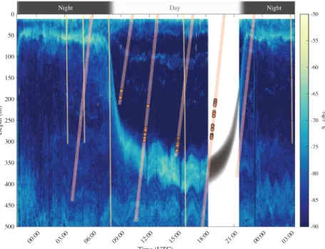
Figure 1. Time series of the mean volume backscattering strength (Sv) at 38 kHz measured from the pole-mounted echo sounder at the NAAMES station located at 44◦21.838′N, 43◦21.503′W occupied from 5 September 2017 21:00 to
7 September 2017 3:00 UTC. Another acoustic frequency (120 kHz) and other stations with float-acoustics matchups are presented in the supporting information. The yellow lines correspond to the downcast of the CTD and the UVP deployed from the ship. The orange lines are the upcasts of the float, and orange circles superimposed on the profiles are FDOM spikes. Note that the first, third, and fifth orange lines are profiles of the floats from the following day. The data from these float profiles are presented in Figure 2. The slopes of the lines correspond to the profiling speed (0.08 m/s for the float and 0.5 m/s for the CTD). No acoustic backscatter was collected between 18:12 and 21:29, the gray shape indicates an estimated depth of the main DVM scattering layer, and the timing was estimated from the DVM observed at other NAAMES stations. The first 10 m of the data are removed to mask near-field effects in the acoustics signal.
3. Results and Discussion
3.1. NAAMES Observations
To illustrate the hypothesis that mesopelagic organisms are at the origin of spike layers in float profiles, we showcase one of the three stations for which we have collocated float data and ship observations. At the case study station (Figure 1), acoustic backscattering at 38 kHz reveals the timing and depth variability of the DVM of organisms from ∼50 m at night to ∼350 m during daytime. This location is also characterized by a nonmigratory deep scattering layer (DSL) observed between 400 and 550 m. Observations collected by the 120-kHz transducer, which are better suited for detection of smaller organism but limited to the upper 200 m of the water column, also show the migrating layer with returns magnitudes slightly higher than those at 38 kHz (1.7 ± 5.7 dB). The location of deep and surface scattering layers detected with the UVP data is consistent with the ones from the acoustic backscatter: During nighttime, higher abundances of zooplankton are observed in the upper 200 m with a peak at 50 m matching the acoustic migrating layer, while during daytime, higher abundances of zooplankton are observed at depth (Figure 2c). Layers of FDOM and bbp spikes were detected in float profiles during daytime (including dawn and dusk) at depths slightly shallower than the ones of the DSL observed with the acoustic (Figure 1) and the UVP (Figure 2).
From the concurrent observations of bio-optical float profiles and ship-based acoustics of the NAAMES expeditions, three matchups had spike layers in float FDOM profiles (15%) and five matchups had individual spikes in float FDOM profiles (25%, supporting information). The analysis revealed that layers of FDOM and bbpspikes were always in the presence of a strong DVM but that not all strong DVM were associated with layers of spikes. Two patterns emerge from our limited data set: (1) The depth of the spike layers or individual spikes from floats is correlated with the depth of the diel migrating acoustics layer, while (2) the depth of the spike layers is mismatched from the depth of the acoustically measured scattering layer, typically at a shallower depth (on average 42 m above, but up to 80 m).
Geophysical Research Letters
10.1029/2019GL086088
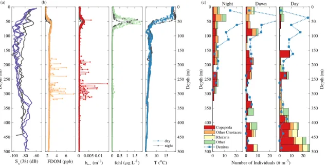
Figure 2. Profiles of the float, the acoustics, and the UVP at the same station presented in Figure 1. (a) Profiles of acoustic backscattering at 38 kHz (Sv(38)) from the ship. (b) Profiles of fluorescent dissolved organic matter (FDOM), particulate backscattering (bbp), chlorophyll a fluorescence (fchl), and
temperature (from left to right) from the float (WMO 5903108) deployed upon arrival on station showcased (Figure 1). Black lines represent to nighttime profiles while colored lines (purple, orange, red, green, and blue) correspond to daytime profiles. The time of the acoustic profiles match exactly with the time of the float profile. (c) Profiles of Copepoda (red), other Crustacea (orange), Rhizaria (yellow), other zooplankton (Annelida, Chaetognatha, Cnidaria, and unidentifiable; green), and detritus (blue lines) binned by 25 m observed by the UVP deployed from the ship. The night profile (left) is an average of the first, second, and fifth casts on station, while the dawn (middle) and day (right) profiles are based on a single cast. Some detritus concentrations are out of scale (night cast 41 particles/m3and dawn cast 35 particles/m3).
Several hypotheses could be brought forward to explain these observations. The depth offset could originate from our observational method due to (1) distance between ship and float, (2) difference in sampling time, (3) deepening of the acoustic layer due to the ship's presence, and/or (4) the float observing a subset of the migrating mesopelagic population. The first two hypotheses could explain why the depths are not consistent but not the presence of a consistent bias. The third hypothesis is unlikely as, to our knowledge, no deepening of scattering layers at such depths was reported (De Robertis & Handegard, 2013; De Robertis et al., 2019; Ona et al., 2007; Peña, 2019). The fourth hypothesis cannot be rejected and is discussed further below. Multiple studies have shown that organisms' size, species richness, and community composition vary with depth. Distinct species assemblages are present at different depths (Kosobokova et al., 2011; Kosobokova & Hopcroft, 2010; Sommer et al., 2017; Steinberg, Cope, et al., 2008; Steinberg, Van Mooy, et al., 2008; Vinogradov, 1970). NAAMES echograms partially illustrate this community's stratification; for example, in Figure 1, four layers of varying intensities can be observed during the daytime, two very thin layers at 100 and 150–200 m, respectively, and two wider layers at 300 to 400 m and 400 to 550 m. None of the observa-tional methods captures the full size range of mesopelagic organisms, rather each method is better suited for a specific size range and type of organisms (Vinogradov, 1997). The acoustic frequencies used here are more sensitive to larger organisms (13 and 39 mm) while the UVP is designed for organisms larger than 0.6 mm (Picheral et al., 2010), suggesting that the depth mismatch between the float and the ship-based observations could result from the stratification of communities of organisms with depth. As the organisms observed at the origin of the spike layer are shallower than the acoustics scattering layer, they are likely to be smaller. Ohman and Romagnan (2016) reported that the vertical distribution shallows progressively with decreasing copepod body size. Thus, the spike layer observed by the float is likely caused by a narrow subset of mesopelagic organisms not prominent in the UVP images and the acoustics scattering.
3.2. Light Attraction of Mesopelagic Organisms
When floats are profiling above 1,000 m, the LED (UV, blue, and red) of the bio-optical sensors is con-tinuously blinking and potentially attracting mesopelagic organisms. Positive phototaxis is well known for mesopelagic organisms; in fact, light traps are commonly used to sample marine biodiversity at depth
(McLeod & Costello, 2017). This positive phototaxis has also been observed with similar bio-optical sensors in coastal environments (Tanaka et al., 2019).
If mesopelagic organisms are attracted to the floats, are they able to reach the light source? When considering the average ascent rate of floats (∼0.08 m/s), it is plausible to assume that some species of zooplankton and other mesopelagic fish are capable of keeping up with floats. Estimated DVM speeds of mesopelagic organisms based on the acoustic data are 0.06 ± 0.01 m/s upward and downward (consistent with Bianchi & Mislan, 2016), and the observed active swimming speeds of Crustaceans and micronekton range from 0.02 to 0.10 m/s and from 0.025 to 0.30 m/s, respectively (Ignatyev, 1997).
In contrast to the float profiles, no spike layers were observed in the particulate attenuation (cp), bbp, and fchl deployed on the CTD Rosette deployed at the same station. A few individual spikes were observed in cp and bbpat 150–250 m and 75 m, respectively, at ∼3:00 UTC, but their depths were not associated with DVM scattering layer, and no spikes were observed in the fchl profile from the CTD Rosette. The CTD Rosette and associated sensors with its twenty-four 12-L bottles displaces a considerable volume of water while traveling down and up at speeds significantly faster than floats (0.5–1 m/s). This likely prevents mesopelagic organ-isms from being able to reach the sensors if attracted to them, especially with the strong shear surrounding the CTD package. These results suggest that the floats are not measuring ambient animal concentration but rather that of mesopelagic organisms attracted to the lights of the bio-optical sensors.
Furthermore, a comparison of the pairs of upcast and downcast of the PROVOR floats (only platform for which downcast data can be recorded) in the western North Atlantic (n = 31) indicates that downcasts tend to have twice as many spikes as upcasts. Given that the PROVOR downcasts are significantly slower than the upcasts (0.04 m/s slower on average) with the same sampling frequency suggest that the elements at the origin of the spikes are staying in front of the sensor, which further supports the light attraction hypothesis. However, this comparison also showed that for upcast and downcast performed within 2 hr (n = 8), the depth of the layers was not significantly different. Therefore the phototactic behavior is not sufficient to explain the depth mismatch between the floats and the acoustics.
3.3. The Origin of the Spikes
While the present results strongly suggest that layers of FDOM or bbpspikes are associated with DVM mesopelagic organisms, the stability of the sensor was assessed to rule out any electronic noise. We then attempt to narrow the variety of organisms at the origin of the spikes.
The sensors used with the BGC-Argo floats (WetLabs ECO-MCOMS or ECO-FLBBCD) have been exten-sively characterized (Carroll et al., 2005; Cetini ´c et al., 2009; Sullivan et al., 2013; Twardowski et al., 2007) and have been found to be susceptible to power surge, submersion, and electromagnetic fields (M. Slivkoff, personal communication). Since the majority of profiles from many different platforms does not contain any FDOM, bbp, or fchl spikes and there is no evidence of the phenomenon listed above, we excluded sensors and platform effects as a source of the spikes observed. We then tested if spikes of similar intensities could be produced by zooplankton using sensors similar to the one mounted on the float (supporting information). Like Tanaka et al. (2019), who used cameras looking at an fchl and bbpsensor, we confirmed that spikes in FDOM, bbp, and fchl could originate from zooplankton. Spikes in backscattering have long been associated with the presence of large particles. Spikes in FDOM can be explained by the fact that fluorescent proteins are possessed by a range of marine organisms and that both humic- and amino acid-like fluorescence are pro-duced by zooplankton grazing and excretion (Stedmon & Cory, 2014). Spikes observed in fchl co-occurring occasionally with the layers of spikes observed in FDOM and bbpchannels are harder to explain. A possible explanation could be the fluorescence from the gut of the zooplankton. However, it would likely be observed only for a short period (several hours) after the time of grazing which isn't the case in our data set. Spikes in fchl could also be caused by the same fluorescent compounds seen by the FDOM sensor (Xing et al., 2017) or by an out of band response given the near saturation of the backscattering channel when measuring spikes which uses the same detector but a different light source.
To identify the organisms that were associated with the observed spikes, we analyzed the community com-position of zooplankton observed with the UVP, the size of the organisms observed by the acoustic, and the community composition of mesopelagic fish sampled with the IKMT net. During the case study station, the zooplankton population was highly dominated by Copepoda and Euphausiids (Figure 2c) with most living organisms seen by the UVP having a Ferret diameter>5 and <25 mm. The acoustics used to observe the
Geophysical Research Letters
10.1029/2019GL086088
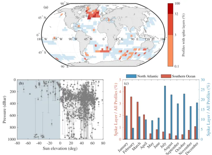
Figure 3. Analysis of BGC-Argo floats with a profiling resolution greater than 1 observation/3 dBar. (a) Locations of float profiles in a 5×5 grid; blue areas indicate the presence of float profiles, and red areas indicate the percentage of profiles withbbpspike layers. (b) Average depth ofbbpspike layer as function of the sun elevation; the error bars correspond to the depth of the shallowest and the deepest spike of the layer. Replacing the sun elevation with PAR measured by the floats equipped with such sensors does not change the pattern significantly (not shown). (c) Number of profiles withbbpspike layers normalized by the total number of profiles in a region per month; the blue histogram is for North Atlantic area, while the red histogram corresponds to the Southern Ocean. Additional information regarding the statistics of the spike layers can be found in the supporting information.
DVM layer was mainly sensitive to organisms with a length of 1 and 4 cm. The samples of the IKMT net, targeting the DSL layer and therefore containing both DVM and non-DVM organisms, were dominated by Myctophids(Diogenichthys atlanticus, Benthosema glaciale, and Myctophym punctatum) during stations of NAAMES 3 with spike layers and by Bristlemouths (Cyclothone pseudopallida) and Penaeidae during the stations of NAAMES 2 with spike layers. These organisms had lengths ranging from 2 to 11 cm. While we could characterize the larger dominant taxa present in the water column, we could not identify the subset of smaller organisms likely at the origin of the spike layers.
3.4. BGC-Argo Observations
Analyses of FDOM and bbpspikes from the broader BGC-Argo database (Figure 3) revealed the following patterns: (1) Layers of spikes were mainly observed at greater depth during daytime while closer to the sur-face during nighttime, (2) layers of spikes are more abundant from the end of spring to early fall in North Atlantic and similar seasons in the Southern Ocean, and (3) layers of spikes are observed primarily in North Atlantic and secondarily in the Southern Ocean. The observations in the North Atlantic are consistent with the current understanding of zooplankton life cycle in this basin: enhanced activity during the phytoplank-ton spring bloom and summer followed by a reduced activity and deepening (diapause) during the winter (Colebrook, 1982; Falkenhaug et al., 1997; Heath, 2000; Miller & Wheeler, 2012).
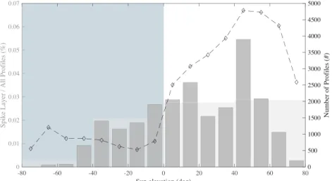
In addition, fewer profiles with a layer of spikes are observed at night than during the day (Figure 4). Perhaps, feeding, one of the primary reasons for DVM (Hays, 2003), could explain the reduction in the phototactic behavior of the taxa responsible for the spike layer. Few profiles are available in the tropics preventing any
Figure 4. Number of spike layer events normalized by sampling effort (number of profiles) as a function of the sun
elevation (zenith angle) (gray histogram). Dark gray histograms correspond to 10◦bins, and lighter histograms in the background correspond to 40◦bins. The total number of float profiles as a function of sun elevation is overlaid as a dashed black line. Negative sun elevation correspond to nighttime while positive sun elevation correspond to daytime.
strong conclusions about this area; only four spike layers were observed in the tropics or subtropics. Still, the normalized (i.e., accounting for sampling effort) number of profiles with spikes is lowest in the tropics and subtropics compared to other parts of the ocean (0.16% vs. 2.6%).
3.5. Other Considerations
We have applied the algorithm developed to automatically detect the presence of spike layers in bio-optical profiles. It performed well in identifying spike layers where layers were recognized visually (Table S1) with FDOM and bbpprofiles but was not reliable for fchl profiles (supporting information and section 3.3). The algorithm offers a way to resolve the source of the bbpspikes; randomly distributed spikes of bbpwhich are not accompanied by FDOM spikes are likely due to sinking aggregates (Briggs et al., 2011), while bbpspikes grouped in layers accompanied by FDOM spike layers are likely due to mesopelagic organisms. Thus, mount-ing FDOM sensors on profilmount-ing floats can help distmount-inguish sources of bbpspikes in float profiles. Nonetheless, the method proposed on floats without FDOM channels works well (identifying correctly layers with a probability>94%). We also recommend to visually inspect and validate each spike layers found.
The results in Figure 3 are likely biased by additional factors: (1) The excitation wavelength of the optical sensors affects the number of spike layer observed: Floats with a backscattering channel at 532 nm (8,093 profiles in the BGC-Argo database) exhibited 50% more spike layers than the other floats in North Atlantic. (2) The profiling frequency: several PROVOR floats from the BGC-Argo array have been set up to profile on a diel basis at times during which the spike layers were prominent which significantly increased the number of spike layers observed. It also allows to observe DVM cycles directly from a float (Boyd et al., 2019). The frequency of spikes in optical signals is tightly linked to the sampling frequency of the sensors. Briggs et al. (2011) recommended having>200 sampling points within a 50-m interval for addressing single spike events due to aggregates. Here, the spike layers of interest are likely due to phototactic organisms; therefore, a lower sampling frequency seems sufficient. The positive phototaxis suggests that bio-optical sensors must be continuously sampling in order to detect spikes as organisms are less likely to swim toward a sensor flashing at low frequency (e.g., once every 30 s). The majority of spike layers are observed with sampling resolution >1 observation/2 dBar. On the other end, no spike layers could be identified on floats with low sampling resolution<1 observation/5 dBar. De facto, this has filtered out the use of APEX BGC-Argo floats (24,873 profiles) from this analysis (see supporting information). The float WMO 5903108, presented in Figures 1 and 2, was set up to sample discretely from a 1,000 to 100 dBar with the bio-optical sensor continuously running (personal communication with Sea-Bird Scientific) resulting in 1–1.5 observations/dBar which was sufficient to detect the presence of mesopelagic organisms with 2 to 18 spikes/50 dBar. Based on this analysis, we recommend that to consistently detect spike layers, floats should profile at a speed<0.08 m/s (i.e., mesopelagic organisms can keep up with the floats), with a sampling resolution>1 observation/dBar
Geophysical Research Letters
10.1029/2019GL086088
(e.g., the bio-optical sensor continuously sampling above 1,000 m), and for the purpose of studying the DVM, floats should profile several times a day.
4. Conclusions
Multiple collocated observations during the NAAMES campaigns and from the BGC-Argo data set show diel variations in the depth of the spike layers that are detected by bio-optical sensors. This pattern is con-sistent with DVM of zooplankton and mesopelagic fish and suggests that a subset of mesopelagic organisms are attracted to the light generated by the bio-optical sensors that are mounted on the floats. Their presence particularly impacted channels designed to measure FDOM and bbp. While the exact organism(s) that gen-erate the spike layers is uncertain, concurrent observations from the UVP and IKMT suggest that Copepoda, Euphausiids, Myctophids, and/or Bristlemouths were present in the water column. As part of this analysis, a novel method was developed for the detection of spike layers in FDOM or bbpprofiles allowing to distinguish the types of particles at the origin of bbpspikes (aggregates or zooplankton). This method can be applied to other slow profiling platforms with high-resolution bio-optical sensors such as gliders or wire-walkers. For the first time, BGC-Argo floats can be used to obtain information on organisms other than phytoplank-ton, adding higher trophic levels to their sensing capability by providing an opportunity to confirm the presence of specific DVM organisms. Furthermore, this type of analysis provides a unique opportunity to study organisms not prominent in current acoustic data sets, with associated hydrographic variables. We encourage future work to identify the specific taxa at the origin of the spike layers. In the near future, floats equipped with cameras (Hydroptic, UVP6-LP) and active acoustics sensors (miniature sonar, Goulet et al., 2019) provide a promising direction to further study these organisms.
References
Abràmoff, M. D., Magalhães, P. J., & Ram, S. J. (2004). Image processing with ImageJ. Biophotonics International, 11(7), 36–41. Behrenfeld, M. J., Moore, R. H., Hostetler, C. A., Graff, J., Gaube, P., Russell, L. M., et al. (2019). The North Atlantic Aerosol and Marine
Ecosystem Study (NAAMES): Science motive and mission overview. Frontiers in Marine Science, 6, 122.
Benoit-Bird, K. J., Patrick Welch, T., Waluk, C. M., Barth, J. A., Wangen, I., McGill, P., et al. (2018). Equipping an underwater glider with a new echosounder to explore ocean ecosystems. Limnology and Oceanography: Methods, 16(11), 734–749.
Bianchi, D., & Mislan, K. A. S. (2016). Global patterns of diel vertical migration times and velocities from acoustic data. Limnology and
Oceanography, 61(1), 353–364.
Bishop, J. K. B., Calvert, S. E., & Soon, M. Y. S. (1999). Spatial and temporal variability of POC in the northeast Subarctic Pacific. Deep Sea
Research Part II: Topical Studies in Oceanography, 46(11-12), 2699–2733.
Bishop, J. K. B., & Wood, T. J. (2008). Particulate matter chemistry and dynamics in the twilight zone at VERTIGO ALOHA and K2 sites.
Deep Sea Research Part I: Oceanographic Research Papers, 55(12), 1684–1706.
Bittig, H., Wong, A., Plant, J., & CORIOLIS-ADMT (2018). BGC-Argo synthetic profile file processing and format on Coriolis GDAC. Ifremer. Boyd, P. W., Claustre, H., Levy, M., Siegel, D. A., & Weber, T. (2019). Multi-faceted particle pumps drive carbon sequestration in the ocean.
Nature, 568(7752), 327–335.
Briggs, N., Perry, M. J., Cetini ´c, I., Lee, C., D'Asaro, E., Gray, A. M., & Rehm, E. (2011). High-resolution observations of aggregate flux during a sub-polar North Atlantic spring bloom. Deep Sea Research Part I: Oceanographic Research Papers, 58(10), 1031–1039. Burt, W. J., & Tortell, P. D. (2018). Observations of zooplankton diel vertical migration from high-resolution surface ocean optical
measurements. Geophysical Research Letters, 45, 13,396–13,404. https://doi.org/10.1029/2018GL079992
Carroll, M., Chigounis, D., Gilbert, S., Gundersen, K., Hayashi, K., Janzen, C., et al. (2005). Performance verification statement for the WET Labs ECO FLNTUSB fluorometer. Alliance for Coastal Technologies, ACT VS07-06.
Cetini ´c, I., Toro-Farmer, G., Ragan, M., Oberg, C., & Jones, B. H. (2009). Calibration procedure for Slocum glider deployed optical instruments. Optics Express, 17(18), 15420.
Claustre, H., Johnson, K. S., & Takeshita, Y. (2020). Observing the global ocean with biogeochemical-Argo. Annual Review of Marine Science,
12(1), 23–48.
Colebrook, J. M. (1982). Continuous plankton records: Seasonal variations in the distribution and abundance of plankton in the North Atlantic Ocean and the North Sea. Journal of Plankton Research, 4(3), 435–462.
Dall'Olmo, G., & Mork, K. A. (2014). Carbon export by small particles in the Norwegian Sea. Geophysical Research Letters, 41, 2921–2927. https://doi.org/10.1002/2014GL059244
De Robertis, A., & Handegard, N. O. (2013). Fish avoidance of research vessels and the efficacy of noise-reduced vessels: A review. ICES
Journal of Marine Science, 70(1), 34–45.
De Robertis, A., & Higginbottom, I. (2007). A post-processing technique to estimate the signal-to-noise ratio and remove echosounder background noise. ICES Journal of Marine Science, 64(6), 1282–1291.
De Robertis, A., Lawrence-Slavas, N., Jenkins, R., Wangen, I., Mordy, C. W., Meinig, C., et al. (2019). Long-term measurements of fish backscatter from Saildrone unmanned surface vehicles and comparison with observations from a noise-reduced research vessel. ICES
Journal of Marine Science, 76, 2459–2470.
Estapa, M. L., Feen, M. L., & Breves, E. (2019). Direct observations of biological carbon export from profiling floats in the subtropical North Atlantic. Global Biogeochemical Cycles, 33, 282–300. https://doi.org/10.1029/2018GB006098
Falkenhaug, T., Tande, K., & Semenova, T. (1997). Diel, seasonal and ontogenetic variations in the vertical distributions of four marine copepods. Marine Ecology Progress Series, 149(1-3), 105–119.
Francois, R. E., & Garrison, G. R. (1982). Sound absorption based on ocean measurements. Part II: Boric acid contribution and equation for total absorption. The Journal of the Acoustical Society of America, 72(6), 1879–1890.
Acknowledgments
We thank M. Behrenfeld and C. Hoestler for leading the NAAMES campaigns, M. Picheral for processing the UVP data set, J. Runge, and A. Poteau for valuable exchanges, and the crew of the R/V Atlantis. We appreciate the help from Melissa Omand and Karen Stamieszkin on the experiment involving zooplankton and FDOM sensors. We thank the two anonymous reviewers for their constructive comments and suggestions which have led to an improved manuscript. This work was founded by the National Atmospheric and Space Administration (NASA) Grant NNX15AE67G. Della Penna is grateful for the support of the Applied Physics Laboratory Science and Engineering Enrichment Development (SEED) fellowship and the European Union's Horizon 2020 research and innovation program under the Marie Sklodowska-Curie Grant agreement 749591. This study is a contribution to remOcean (European Research Council, Grant agreement 246777), REFINE (European Research Council, Grant agreement 834177), AtlantOS (European Union's Horizon 2020 research and innovation program, Grant 2014-633211), SOCLIM (BNP Foundation), and SOCCOM (NASA Grants NNX14AP49G and 80NSSC19K0001) projects. The data presented are part of the NASA NAAMES project and BGC-Argo; it is shared on https://seabass.gsfc.nasa. gov/archive/UWASH/gaube/ NAAMES/ (echo sounder), https:// ecotaxa.obs-vlfr.fr/prj/637 (UVP), http://misclab.umeoce.maine.edu/ floats/ (NAAMES floats), and http:// www.argo.ucsd.edu/Acknowledging_ Argo.html GDAC (BGC-Argo floats). Source codes are available online (https://github.com/OceanOptics/ FloatSpikeAnalysis/).
Goulet, P., Guinet, C., Swift, R., Madsen, P. T., & Johnson, M. (2019). A miniature biomimetic sonar and movement tag to study the biotic environment and predator-prey interactions in aquatic animals. Deep Sea Research Part I: Oceanographic Research Papers, 148(May), 1–11.
Hays, G. C. (2003). A review of the adaptive significance and ecosystem consequences of zooplankton diel vertical migrations.
Hydrobiolo-gia, 503(1-3), 163–170.
Heath, M. (2000). Winter distribution of Calanus finmarchicus in the Northeast Atlantic. ICES Journal of Marine Science, 57(6), 1628–1635. Ignatyev, S. M. (1997). Pelagic fishes and their macroplankton prey: Swimming speeds. In Forage Fishes in Marine Ecosystems, American
Fisheries Society(pp. 31–39). University of Alaska Fairbanks.
Kosobokova, K. N., & Hopcroft, R. R. (2010). Diversity and vertical distribution of mesozooplankton in the Arctic's Canada Basin. Deep Sea
Research Part II: Topical Studies in Oceanography, 57(1-2), 96–110.
Kosobokova, K. N., Hopcroft, R. R., & Hirche, H.-J. (2011). Patterns of zooplankton diversity through the depths of the Arctic's central basins. Marine Biodiversity, 41(1), 29–50.
Llort, J., Langlais, C., Matear, R., Moreau, S., Lenton, A., & Strutton, P. G. (2018). Evaluating Southern Ocean carbon eddy-pump from biogeochemical-Argo floats. Journal of Geophysical Research: Oceans, 123, 971–984. https://doi.org/10.1002/2017JC012861
McDougall, P. M., & Trevor, J. B. (2011). Getting started with TEOS-10 and the Gibbs Seawater (GSW) oceanographic toolbox. SCOR/IAPSO WG127.
McLeod, L. E., & Costello, M. J. (2017). Light traps for sampling marine biodiversity. Helgoland Marine Research, 71(1), 2.
Medwin, H. (1975). Speed of sound in water: A simple equation for realistic parameters. The Journal of the Acoustical Society of America,
58(6), 1318–1319.
Miller, C. B., & Wheeler, P. A. (2012). Population biology of zooplankton. Biological oceanography (pp. 158–180). Hoboken, UK: John Wiley & Sons.
Ohman, M. D., Davis, R. E., Sherman, J. T., Grindley, K. R., Whitmore, B. M., Nickels, C. F., & Ellen, J. S. (2019). Zooglider: An autonomous vehicle for optical and acoustic sensing of zooplankton. Limnology and Oceanography: Methods, 17(1), 69–86.
Ohman, M. D., & Romagnan, J.-B. (2016). Nonlinear effects of body size and optical attenuation on diel vertical migration by zooplankton.
Limnology and Oceanography, 61(2), 765–770.
Ona, E., Godø, O. R., Handegard, N. O., Hjellvik, V., Patel, R., & Pedersen, G. (2007). Silent research vessels are not quiet. The Journal of
the Acoustical Society of America, 121(4), EL145–EL150.
Peña, M. (2019). Mesopelagic fish avoidance from the vessel dynamic positioning system. ICES Journal of Marine Science, 76(3), 734–742. Picheral, M., Colin, S., & Irisson, J.-O. (2017). EcoTaxa, a tool for the taxonomic classification of images.
Picheral, M., Guidi, L., Stemmann, L., Karl, D. M., Iddaoud, G., & Gorsky, G. (2010). The Underwater Vision Profiler 5: An advanced instrument for high spatial resolution studies of particle size spectra and zooplankton. Limnology and Oceanography: Methods, 8(9), 462–473.
Reda, I., & Andreas, A. (2004). Solar position algorithm for solar radiation applications. Solar Energy, 76(5), 577–589.
Roesler, C., Uitz, J., Claustre, H., Boss, E., Xing, X., Organelli, E., et al. (2017). Recommendations for obtaining unbiased chlorophyll estimates from in situ chlorophyll fluorometers: A global analysis of WET Labs ECO sensors. Limnology and Oceanography: Methods,
15(6), 572–585.
Ryan, T. E., Downie, R. A., Kloser, R. J., & Keith, G. (2015). Reducing bias due to noise and attenuation in open-ocean echo integration data. ICES Journal of Marine Science: Journal du Conseil, 72(8), 2482–2493.
Schmechtig, C., Organelli, E., Poteau, A., Claustre, H., & D'Ortenzio, F. (2017). Processing BGC-Argo CDOM concentration at the DAC level. Ifremer.
Schmechtig, C., Poteau, A., Claustre, H., D'Ortenzio, F., & Boss, E. (2015). Processing Bio-Argo chlorophyll-a concentration at the DAC Level. Ifremer.
Schmechtig, C., Poteau, A., Claustre, H., D'Ortenzio, F., Dall'Olmo, G., & Boss, E. (2018). Processing BGC-Argo particle backscattering at the DAC level. Ifremer.
Sommer, S. A., Van Woudenberg, L., Lenz, P. H., Cepeda, G., & Goetze, E. (2017). Vertical gradients in species richness and community composition across the twilight zone in the North Pacific Subtropical Gyre. Molecular Ecology, 26(21), 6136–6156.
Stedmon, C. A., & Cory, R. M. (2014). Biological origins and fate of fluorescent dissolved organic matter in aquatic environments. In P. Coble, J. Lead, A. Baker, D. M. Reynolds, & R. G. M. Spencer (Eds.), Aquatic organic matter fluorescence (pp. 278–300). Cambridge: Cambridge University Press.
Steinberg, D. K., Cope, J. S., Wilson, S. E., & Kobari, T. (2008). A comparison of mesopelagic mesozooplankton community structure in the subtropical and subarctic North Pacific Ocean. Deep-Sea Research Part II: Topical Studies in Oceanography, 55(14-15), 1615–1635. Steinberg, D. K., & Landry, M. R. (2017). Zooplankton and the ocean carbon cycle. Annual Review of Marine Science, 9(1), 413–444. Steinberg, D. K., Van Mooy, B. A. S., Buesseler, K. O., Boyd, P. W., Kobari, T., & Karl, D. M. (2008). Bacterial vs. zooplankton control of
sinking particle flux in the ocean's twilight zone. Limnology and Oceanography, 53(4), 1327–1338.
Sullivan, J. M., Twardowski, M. S., Ronald, J., Zaneveld, V., & Moore, C. C. (2013). Measuring optical backscattering in water. In A. A. Kokhanovsky (Ed.), Light scattering reviews 7, Springer Praxis Books (pp. 189–224). Berlin, Heidelberg: Springer Berlin Heidelberg. Tanaka, M., Genin, A., Lopes, R. M., Strickler, J. R., & Yamazaki, H. (2019). Biased measurements by stationary turbidity-fluorescence
instruments due to phototactic zooplankton behavior. Limnology and Oceanography: Methods, 17, 505–513.
Twardowski, M. S., Claustre, H., Freeman, S. A., Stramski, D., & Huot, Y. (2007). Optical backscattering properties of the “clearest” natural waters. Biogeosciences, 4(6), 1041–1058.
Vinogradov, M. E. (1970). Vertical distribution of the oceanic zooplankton.
Vinogradov, M. E. (1997). Some problems of vertical distribution of meso- and macroplankton in the ocean. Advances in Marine Biology,
32, 1–92.
Xing, X., Claustre, H., Boss, E., Roesler, C., Organelli, E., Poteau, A., et al. (2017). Correction of profiles of in-situ chlorophyll fluorometry for the contribution of fluorescence originating from non-algal matter. Limnology and Oceanography: Methods, 15(1), 80–93.