HAL Id: tel-01233019
https://tel.archives-ouvertes.fr/tel-01233019
Submitted on 24 Nov 2015HAL is a multi-disciplinary open access archive for the deposit and dissemination of sci-entific research documents, whether they are pub-lished or not. The documents may come from teaching and research institutions in France or abroad, or from public or private research centers.
L’archive ouverte pluridisciplinaire HAL, est destinée au dépôt et à la diffusion de documents scientifiques de niveau recherche, publiés ou non, émanant des établissements d’enseignement et de recherche français ou étrangers, des laboratoires publics ou privés.
Energy balance mathematical model on climate change
Benjamin Keroboto Za’Ngoti Ogutu
To cite this version:
Benjamin Keroboto Za’Ngoti Ogutu. Energy balance mathematical model on climate change. Con-tinental interfaces, environment. Université Pierre et Marie Curie - Paris VI; University of Nairobi, 2015. English. �NNT : 2015PA066224�. �tel-01233019�
Université Pierre et Marie Curie
Université de Nairobi
Ecole doctorale 129
Laboratoire Meteorologie Dynamique
Energy Balance Mathematical model on Climate Change
Par KEROBOTO B.Z. OGUTU
Thèse de doctorat de Météorologie, Oceanographie, Environment
Dirigée par [Fabio D’Andrea, Charles Nyandwi]
Présentée et soutenue publiquement le 25/5/2015
Devant un jury composé de :
P.G.O Weke, director of the School of Mathematics, president Kaveh Madani, professeur, rapporteur,
Charles Nyandwi, professeur, co-Directeur de these,
Fabio D’Andrea, chargé de recherches, co-Directeur de these Michael Ghil, professeur, examinateur.
Wandera Ogana, professeur, examinateur Francis Codron, professeur, examinateur Ganesh Pokhariyal, professeur, examinateur
ii
DEDICATION
This thesis is dedicated to GOD, all my teachers who showed me the beauty of knowledge, my mother ‒ Maria Consolata Nyangige BORORO, my family, and humanity for their support on this journey.
“All men dream, but not equally. Those who dream by night in the dusty recesses of their minds wake in the day to find that it was vanity; but dreamers of the day are dangerous men, for they may act their dream with open eyes, to make it possible. This I did…”
(Seven Pillars of Wisdom by Lawrence TE 2006, p. 7) … Coupled with the full knowledge that:
“A phrase is born into the world both good and bad at the same time. The secret lies in a slight, an almost invisible twist. The lever should rest in your hand, getting warm, and you can only turn it once, not twice.” Isaac Babel, Russian short-story writer, 1894–1941.
(The Yale book of quotations by Shapiro FR 2006, p. 38)
… And:
Everything should be made as simple as possible, but not simpler…
“As far as the laws of mathematics refer to reality, they are not certain; and as far as they are certain, they do not refer to reality.”
iii
ACKNOWLEDGEMENTS
I would like to express sincere thanks to my dynamic and inspirational icons, supervisors, and advisors Dr. Fabio D'ANDREA, Prof. Philippe CIAIS, Dr. Charles NYANDWI, and Prof. Moses Mwangi MANENE for their boundless energy, unstinting attention and support, wise and considered counsel, insightful guidance, a listening ear(s) and patience throughout my endeavour to get this work done. They set high standards for themselves and encouraged me to do the same – to apply knowledge, challenge norms, inspire others, and above all, be accountable for my own decisions and actions.
Much thanks also to Prof. Michael GHIL (Professeur des Universités, Directeur du Département Terre-Atmosphére-Océan, Ecole Normale Supérieure, 24, Rue Lhomond, 75231 Paris Cedex 05 (France)), Prof. Nzioka John MUTHAMA (Metereology Department, School of Physical Sciences, University of Nairobi), Dr. David Williamson (Institute of Research for Development (IRD)), Dr. Jean Albergel (Representative of the French IRD for East Africa), Dr. Fogel-Verton Séverine and NGUEMA Sarah-Ayito (Cooperation Attaché Embassy of France in Kenya) and the School of Mathematics (University of Nairobi) Board of Postgraduate Committee members for taking their time to serve in their various positions. I would also like to appreciate my colleagues at the Department of Statistics and Actuarial Science (DeSAS) and the entire Dedan Kimathi University of Technology (DeKUT) fraternity for their good gestures.
Above all I thank God for the blessing of my family members who were patient and loving throughout the journey infinite deepest gratitude to you Ruth Wambui Za’Ngoti, Alex Ogutu, Valentine Nyangige, Joy Wangari, Lorna Wanjiku, and Fabioh Pasaka.
iv
ABSTRACT
The goal of this study is to build a reduced-complexity model of coupled climate-economy-biosphere interactions, which uses the minimum number of variables and equations needed to capture the fundamental mechanisms involved and can thus help clarify the role of the different variables and parameters. The Coupled Climate-Economy-Biosphere (CoCEB) model described herein takes an integrated assessment approach to simulating global change. By using an endogenous growth module with physical and human capital accumulation, this study considers the sustainability of economic growth, as economic activity intensifies greenhouse gas emissions that in turn cause economic damage due to climate change. Various climate change mitigation policy measures are considered. While many integrated assessment models treat abatement costs merely as an unproductive loss of income, this study considers abatement activities also as an investment in increase of overall energy efficiency of the economy and decrease of overall carbon intensity of the energy system.
One of the major drawbacks of integrated assessment models is that they mainly focus on mitigation in the energy sector and consider emissions from land-use as exogenous. Since greenhouse gas emissions from deforestation and current terrestrial uptake are significant, it is important to include mitigation of these emissions in the biota sinks within integrated assessment models. Several studies suggest that forest carbon sequestration can help reduce atmospheric carbon concentration significantly and is a cost efficient way to curb the prevailing climate change. This study also looks at relevant economic aspects of deforestation control and carbon sequestration in forests as well as the efficiency of carbon capture and storage (CCS) technologies as policy measures for climate change mitigation.
v
Because full realistic coupled climate models are so complex, analyses of the various potential feedbacks between climate, economy, and biosphere have been rather limited. Potentially important mechanisms are better initially described in low or intermediate complexity models.
The CoCEB is a formal framework in which it is possible to represent in a simple way different elements of the coupled system and their interactions. The model developed, being an exercise in simplicity and not a predictive tool for climate change impacts, brings together and summarizes information from diverse literature on climate change mitigation measures and their associated costs, and allows comparing them in a coherent way.
The model is, of course sensitive, to the choice of key parameters and in particular the parameters setting the costs of the different means of climate change mitigation: the parameter values tested span the range of cost values found in literature.
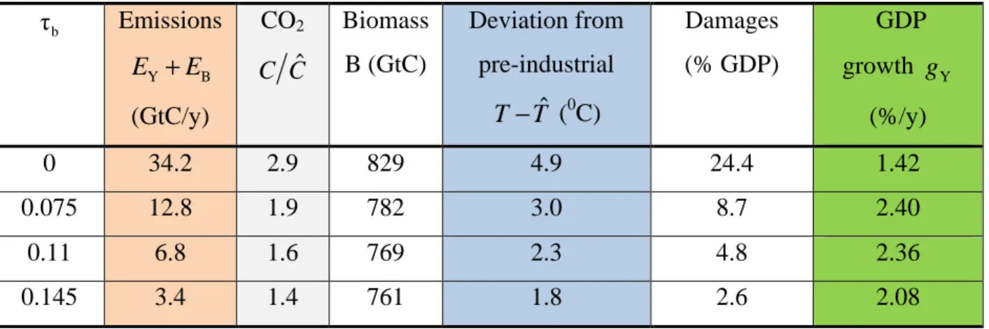
The study shows that: i) investment in low-carbon technologies helps to reduce the volume of industrial carbon emissions, lower temperature deviations, and lead to positive effects in the long term economic growth; ii) low investment in CCS contributes to reducing industrial carbon emissions and to increasing gross domestic product (GDP), but further investment leads to a smaller reduction in emissions, as well as in the incremental GDP growth; iii) enhanced deforestation control contributes to a reduction in both deforestation emissions and atmospheric carbon dioxide concentration, thus reducing the impacts of climate change and contributing to a slight appreciation of GDP growth, an effect that is very small, though, compared to that of low-carbon technologies or CCS; and iv) the results in i) and ii) remain very sensitive to the formulation of technological improvements costs. To the contrary, the results for deforestation control are less sensitive to the formulation of its cost. A large range of hypotheses on these costs appear in the literature, and our modeling framework permitted to span this range and check the
vi
sensitivity of results The sensitivity study is not intended to make precise calibrations; rather, it is meant to provide a tool for studying qualitatively how various climate policies affect the economy.
RÉSUMÉ
L'objectif de cet étude est de construire un modèle de complexité réduite qui intègre les interactions et les rétroactions du système climat-économie-biosphère avec le minimum de variables et d'équations nécessaires afin de rendre les interactions dynamiques entre les différentes variables transparents. Le modèle couplé climat-économie-biosphère (CoCEB) décrit une approche d'évaluation intégrée pour simuler les changements planétaires. En utilisant un module de croissance endogène avec accumulation de capital physique et humaine, cette étude adresse le problème de la durabilité de la croissance économique. L’activité économique intensifie les émissions de gaz à effet de serre qui à leur tour causent des dommages économiques en raison du changement de climat. Diverses mesures de politique d'atténuation du changement climatique sont considérées. Alors que beaucoup IAM (Integrated assessment models) traitent les coûts de réduction des émissions (abatement) simplement comme une perte non productive de revenu, cet étude considère également les activités de réduction des émissions comme un investissement dans l'efficacité énergétique globale de l'économie et dans la diminution de l’ « intensité carbone » globale du système énergétique.
Un des inconvénients majeurs des IAM est qu'ils se concentrent principalement sur le secteur énergétique pour les mesures d’attenuation, et ne tiennent compte des émissions provenant de l'utilisation des terres que comme un forçage exogène. Cependant, les émissions de gaz à effet de serre due au changement de destination du sol, et l’effet de la séquestration de carbone par la terre a sont importantes, l éffet des puits de biota doit donc être considéré. Plusieurs études suggèrent que le piégeage du carbone forestier peut aider à réduire de façon significative la
vii
concentration de carbone atmosphérique et qu’il est un moyen efficace en termes de coût pour freiner le changement climatique. Cette étude se penche donc également sur les aspects économiques de la séquestration de carbone du au contrôle du déboisement dans les forêts, at aussi de l’application généralisée des technologies de capture et stockage du carbone (CCS).
Du moment que les modèles climatiques couplés réalistes sont très complexes, les analyses des diverses rétroactions potentielles entre climat, économie et la biosphère ont été plutôt limitées. Mécanismes potentiellement importants sont mieux initialement décrites dans des modèles de complexité faible ou intermédiaire.
La CoCEB est un cadre formel dans lequel il est possible de représenter de façon simple les différents éléments du système couplé et leurs interactions. Le modèle mis au point, étant un exercice de simplicité et pas un outil de prédiction des impacts du changement climatique, rassemble et résume les différentes données trouvées dans la littérature sur les mesures de mitigation et les coûts y afférents, et permet de les comparer de façon cohérente.
Le modèle est sensible au choix des paramètres, en particulier au paramètres définissant les coûts des différents moyens d'atténuation de changement climatique: on a testé les valeurs des paramètres couvrant la gamme des valeurs de coût trouvé dans la littérature.
L'étude montre que: i) investissements dans les technologies à faible intensité de carbone contribue à réduire le volume des émissions de carbone industriel, réduire les écarts de température et entraîner des effets positifs de la croissance économique à long terme; ii) un faible investissement dans les CCS contribue à réduire les émissions de carbone industriel et à une augmentation de la croissance du PIB, mais un investissement supplémentaire a un effet inverse et diminue la réduction dans les émissions ainsi que l'incrément de croissance du PIB; iii) augmentation du contrôle de la déforestation contribue à réduire les émissions de la déforestation et concentration de CO2 atmosphérique, ce qui réduit les impacts du changement climatique. Ces éléments
viii
contribuent à une légère appréciation de la croissance du PIB, mais cela reste très faible par rapport à l'effet des technologies à faible intensité carbonique ou CCS; iv) les résultats en i) et ii) restent très sensibles à la formulation du coût des améliorations technologiques. Un large éventail d'hypothèses sur ces coûts se trouve dans la littérature, notre modèle permet d'étendre cette gamme et vérifier la sensibilité des résultats. À l'inverse, les résultats pour le contrôle de la déforestation sont moins sensibles à la formulation de son coût. L'étude de sensibilité ne représente pas un calibrage précis ; au contraire, il est destiné à fournir un outil pour étudier qualitativement comment diverses politiques climatiques influent sur l'économie.
ix
TABLE OF CONTENTS
DECLARATION ... Erreur ! Signet non défini. Declaration by the candidate ... Erreur ! Signet non défini. Declaration by supervisors ... Erreur ! Signet non défini.
DEDICATION ... ii
ACKNOWLEDGEMENTS ... iii
ABSTRACT ... iv
RÉSUMÉ ... vi
TABLE OF CONTENTS ... ix
LIST OF FIGURES ... xii
LIST OF TABLES ... xiii
OPERATIONAL DEFINATIONS OF TERMS AND CONCEPTS ... xiv
ABBREVIATIONS AND ACRONYMS ... xviii
INTRODUCTION ... 1
1.1 Background to the problem ... 1
1.2 Statement of the problem and justification ... 4
1.3 Objectives of the study ... 5
1.4 Significance of the study ... 6
1.5 Research methodology and outline of the study ... 6
LITERATURE REVIEW ... 9
2.1 Climate change and climate variability ... 9
2.2 Integrated assessment modelling (IAM) ... 10
2.2.1 The emergence of IAMs as a science-policy interface ... 10
x
2.2.3 Application of integrated assessment models ... 12
2.2.4 Challenges for IAM studies ... 14
2.2.5 Improvements of IAMs ... 15 2.2.6 This study ... 17 MODEL DESCRIPTION ... 21 3.1 Climate module ... 21 3.2 Economy module ... 22 3.3 Industrial CO2 emissions ... 25
3.3.1 Inclusion of CCS in the industrial CO2 emissions equation ... 28
3.3.2 Cost of CCS ... 29
3.3.3 Damage function ... 30
3.4 Inclusion of a Biosphere module: CO2-biomass interactions ... 32
3.4.1 Carbon flux from deforestation and deforestation control ... 33
3.4.2 Cost of the deforestation activity ... 34
3.5 Climate change abatement measures ... 36
3.5.1 Abatement policies ... 36
3.5.2 Abatement share ... 37
3.5.3 Deforestation control and afforestation ... 38
3.6 Summary: CoCEB, the Coupled Climate-Economy-Biosphere model ... 39
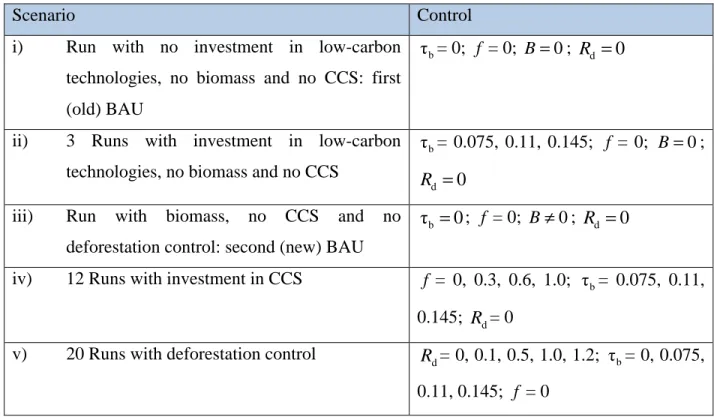
NUMERICAL SIMULATIONS AND ABATEMENT RESULTS ... 44
4.1 Experimental design ... 44
4.2 Integrations without and with investment in low-carbon technologies and with no CCS, biomass or deforestation control ... 46
4.3 Control integration: run with biomass, no CCS and no deforestation control (new BAU) 52 4.4 Using CCS methods but no deforestation control ... 53
xi
4.6 A mix of mitigation measures ... 58
SENSITIVITY ANALYSIS ... 61
5.1 Damage function parameters m1 and χ ... 61
5.2 Robustness to changes in the low-carbon abatement efficiency parameter ατ ... 64
5.3 Robustness to changes in the CCS abatement efficiency parameter αω ... 65
5.4 Robustness to changes in the deforestation control cost parameters ... 66
CONCLUSIONS AND WAY FORWARD ... 67
6.1 Summary ... 67
6.2 Discussion ... 69
REFERENCES ... 76
APPENDICES ... 99
Appendix 1: Table of conversions ... 99
xii
LIST OF FIGURES
Figure 1 Schematic of climate-economy-biosphere interactions (see also, Kellie-Smith and Cox
2013)… ………...3
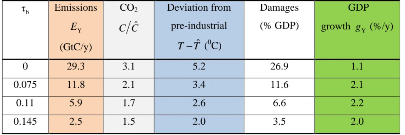
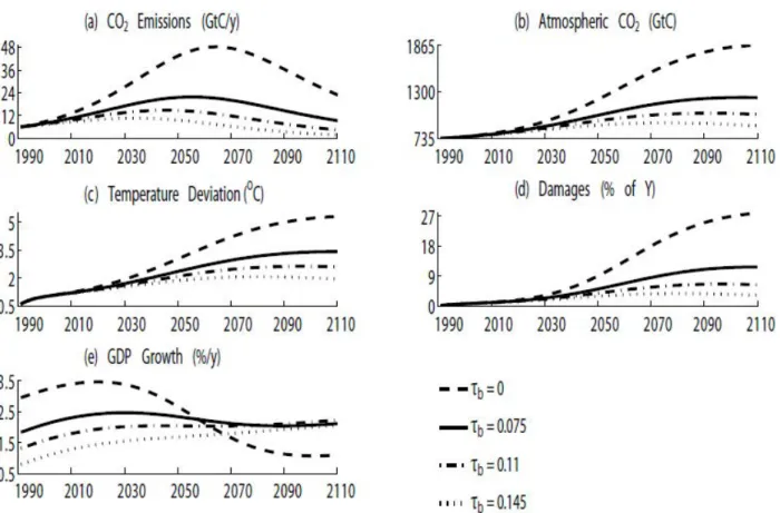
Figure 2 The various modules of the study (see also, Edwards et al. 2005, p. 2, Figure 1.1)...7 Figure 3 Evolution of several CoCEB model variables in time, for abatement shares τ that range b
from 0.0 (no abatement) to 0.145; see legend for curves, with τ = 0 — dashed, b τ = 0.075 — b solid, τ = 0.11 — dash-dotted, and b τ = 0.145— dotted...………...45 b
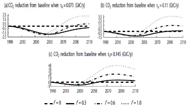
Figure 4 Evolution in time of reduction in CO2 emissions from baseline, for and , and for -values that range from 0 (0 % investment in CCS) to 1.0 (100 % investment in CCS). (a) = 0.075, (b) =0.11, and (c) = 0.145; see legend for curves, with f = 0 — dashed, f = 0.3 — solid, f = 0.6 — dash-dotted, and f = 1.0 — dotted ………...53
Figure 5 GDP growth over time, with biomass module (B≠0), as a function of abatement share values τ between 0.0 (no abatement) and 0.145. (a) b Rd =0 and f = ; panel (b) 0 Rd =0.1 and
0.3
f = ; see legend for curve identification ………...57
Figure 6 GDP growth over time as a function of abatement share values τ between 0.0 and b
0.145; see legend for curve identification, while ατ =1.8, f = , 0 B=0, Rd = . Panels (a, b) 0 m 1
is larger or smaller by 50 % than the value in Tables 1–9; (c, d) same for the nonlinearity
xiii
LIST OF TABLES
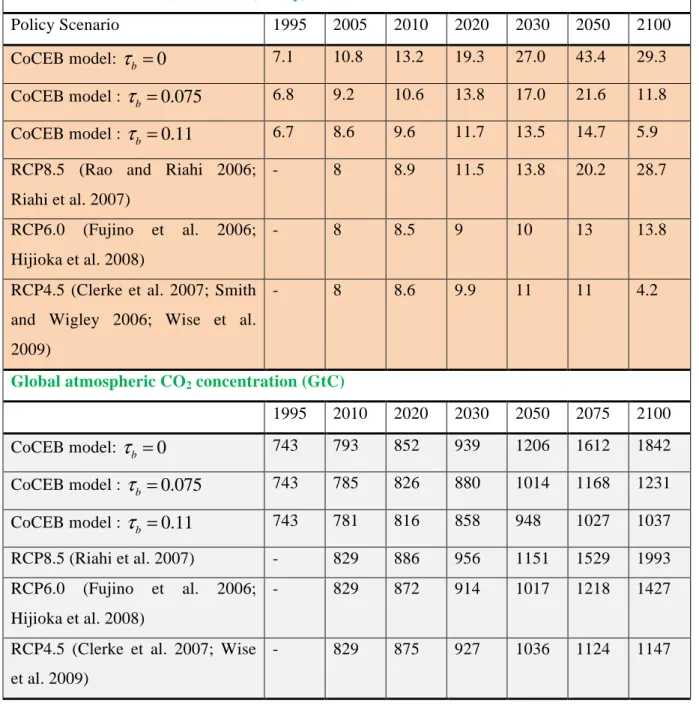
Table 1 List of variables and parameters and their values used………...39 Table 2 The scenarios studied herein……….………...42 Table 3 Variables values for year 2100 for the model without and with investment in low-carbon
technologies: scenarios i) and ii) in Table 2, with χ 2.43= ………...44
Table 4 Per capita abatement costs and damage costs at year 2100, with χ 2.43= ………48
Table 5 Comparison between global results of alternative policies………49
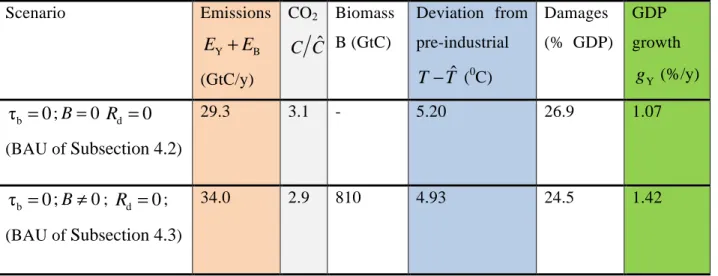
Table 6 Variable values for year 2100 for the model with no biomass (B = 0) and no CCS (f = 0),
i.e. BAU of Table 3, and with no deforestation control but B ≠ 0 (new BAU run)………..50
Table 7 Variable values for year 2100 with deforestation emissions in parenthesis, for the runs
with investment in CCS scenario………...52
Table 8 Variable values for year 2100, with deforestation emissions in parenthesis, for runs with
inclusion of deforestation control scenario………...55
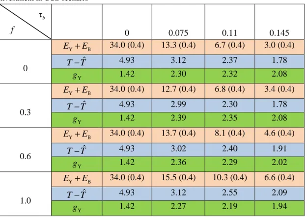
Table 9 Target values of key variables for our policy scenarios at year 2100, with f =0.3 and d 0.1
R = ………...56
Table 10 Policy scenario values at year 2100 with ατ =1.8, f = , 0 B=0, Rd = , varying 0 m , 1
and χ………...60
Table 11 Effect of varying α by year 2100; τ f = , 0 B=0, Rd = , other parameter values as in 0 Table 1………...62
Table 12 Effect of varying α by year 2100; ω B≠0, Rd = , τ0 b= 0.075, and all other parameter
xiv
OPERATIONAL DEFINATIONS OF TERMS AND CONCEPTS
Adaptation Adjustment in natural or human systems to a new or changing environment.Albedo Fraction of solar radiation reflected back by a surface or object, often expressed as a percentage.
Biomass The organic material both above-ground (stem, branches, bark, seeds and foliage) and below-ground (living biomass of life roots), and both living and dead.
Carbon cycle The flow of carbon in various forms (for example, CO2) through the climate
System.
Carbon sequestration
The process through which agricultural and forestry practices remove carbon dioxide (CO2) from the atmosphere.
Climate The statistical description in terms of the mean and variability of relevant quantities (surface temperature, precipitation, wind, etc.) over a period of time ranging from months to thousands or millions of years.
Climate change A change of the state of the climate system that can be identified by changes in the mean and/or variability of its properties and that persists for an extended period, typically decades or longer.
Climate system A complex system consisting of five major components: the atmosphere, the hydrosphere, the cryosphere, the lithosphere, and the biosphere, and the interactions between them.
Climate variability
Variations beyond the mean state and other statistics of the climate on all spatial and temporal scales.
xv
concentration.
Damage function The relation between changes in the climate and reductions in economic
activity relative to the rate that would be possible in an unaltered climate.
Deforestation Those forestry practices or processes that result in a long-term land-use change from forest to agriculture or human settlements or other non-forest uses.
Differential equation
A mathematical equation for a function of one or more independent variables involving the function and its derivatives.
Energy balance The difference between the total incoming and the total outgoing energy. If this balance is positive, warming occurs; if it is negative, cooling occurs. Averaged over the globe and over long time periods of at least 30 years, the balance must be zero. A perturbation of this balance, be it human-induced or natural, is called radiative forcing.
Feedback The phenomenon whereby the output of a system is fed into the input and the
output is subsequently affected.
Forcing The action of an agent outside the climate system (volcanic eruption, solar variation, anthropogenic action, etc.) causing a change in the climate system.
GDP Gross Domestic Product. The value of all goods and services produced (or consumed) within a nation’s borders.
Greenhouse effect
The trapping of heat by greenhouse gases (GHGs) within the surface-troposphere system. An increase in the concentration of GHGs leads to an increased opacity for infrared radiation of the atmosphere.
Integrated assessment
A method of analysis that combines results and models from the physical, biological, economic and social sciences, and the interactions between these
xvi
components, in a consistent framework, to project the consequences of climate change and the policy responses to it.
Kyoto Protocol A United Nations Protocol of the Framework Convention for Climate Change
that aims to reduce anthropogenic emissions of CO2. It sets limits for
anthropogenic CO2 emissions with a view to reducing overall emissions to 5
per cent below 1990 levels by 2008 to 2012. See http://unfccc.int.
Land-use The total of arrangements, activities, and inputs undertaken in a certain land cover type (a set of human actions). The social and economic purposes for which land is managed (e.g., grazing, timber extraction, and conservation).
Land-use change A change in the use or management of land by humans, which may lead to a
change in land cover. Land cover and land-use change may have an impact on the albedo, evapotranspiration, sources and sinks of greenhouse gases, or other properties of the climate system, and may thus have an impact on climate, locally or globally.
Mitigation Technological change and substitution that reduce resource inputs and emissions per unit of output with respect to climate change, mitigation means implementing policies to reduce GHG emissions and enhance sinks.
Parameterization The method of incorporating a process by representation as a simplified
function of some other fully resolved variables without explicitly considering the details of the process.
Photosynthesis The metabolic process by which plants take CO2 from the air (or water) to build
xvii
Radiative forcing A change in the average net radiation at the tropopause — the region between the troposphere and the stratosphere — brought about by changes in either the incoming solar radiation, or in the outgoing infrared radiation. Radiative forcing therefore disturbs the balance that exists between incoming and outgoing radiation. As the climate system evolves over time, it responds to the perturbation by slowly re-establishing the radiative balance.
Reforestation Planting of forests on lands that have previously contained forests but that have been converted to some other use.
Sequestration The process of increasing the carbon content of a carbon reservoir other than the atmosphere. Biological approaches to sequestration include direct removal of carbon dioxide from the atmosphere through land - use change,
afforestation, reforestation, and practices that enhance soil carbon in
agriculture. Physical approaches include separation and disposal of carbon dioxide from flue gases or from processing fossilfuels to produce hydrogen- and carbon dioxide-rich fractions and long-term storage in underground in depleted oil and gas reservoirs, coal seams, and saline aquifers.
Sinks This is term used here to describe agricultural and forestry land that absorbs CO2, the most important global warming gas emitted by human activities. Solar constant The amount of radiation from the Sun incident on a surface at the top of the
atmosphere perpendicular to the direction of the Sun. Currently taken to be 1366 Wm-2 . Note that S can denote both 1366 Wm-2, one quarter of this or the instantaneous top-of-the- atmosphere solar flux at a particular location. Context usually indicates which is meant.
Stefan– Boltzmann constant
s, having a value of 5.67 × 10⁻⁸W m-2K-4, the constant of proportionality in Stefan’s law.
xviii
Stefan’s law This is the relationship between the amount of energy radiated by a body and its temperature and is given by E = sT4 where E is in Wm-2 and s is the Stefan– Boltzmann constant.
Surface air temperature
The temperature of the air near the surface of the Earth, usually determined by a thermometer in an instrument shelter about 1.3 m above the ground.
ABBREVIATIONS AND ACRONYMS
BAU Business-as-UsualC Carbon
CCS Carbon Capture and Sequestration
CDM Clean Development Mechanism
CO2 Carbon dioxide
EBM An Energy Balance Model. Probably the simplest model of the Earth
system, based on the energy balance between the solar energy absorbed from the Sun and the thermal radiation emitted to space by the Earth
UNFCCC The UN Framework Convention on Climate Change. Signed at the UN
Conference on Environment and Development in 1992 and ratified in 1994. The FCCC has defined climate change to be only the human-induced effects (i.e. not natural variability) for its negotiations
GCM A General Circulation Model or Global Climate Model. Initially used with reference to three-dimensional models of the atmosphere alone, the term has come to be loosely used to encompass three-dimensional models of the ocean (OGCMs) and coupled
xix models GEB GHGs Gt GtC IAMs
Global energy balance GreenHouse Gases Gigatonnes
Gigatonnes of Carbon
Integrated Assessment Models
IPCC The Intergovernmental Panel on Climate Change. Established in 1988 and jointly sponsored by United Nations Environmental Programme and World Health Organization. Note that the IPCC is an assessment, not a research organization
KP Kyoto Protocal
NGOs Non-Government Organizations
REDD Reduced Emissions from Deforestation and forest Degradation
TRF Tons of reference fuel
1
CHAPTER 1
INTRODUCTION
1.1 Background to the problem
It is widely accepted that climate change will have major impacts on humankind. Depending on the magnitude of twenty-first century climate change, human societies and ecosystems are expected to be greatly affected by climate change (IPCC 2007b) and in particular by the frequency and intensity of extreme events (e.g., Changnon et al. 1996; Ciais et al. 2005; IPCC 2012a). Negative impacts are expected on water, food, human health and conflict (IPCC 2001b, p. 238; IPCC 2007b) and ultimately economic growth (Dell et al. 2014 and the citations therein; Nordhaus 2008; Stern 2007). Global carbon dioxide (CO2) emissions, which are the largest contributor to
anthropogenic climate change (Farmer and Cook 2013, p. 4; Mokhov et al. 2012; Stern 2008; Stott et al. 2000), have, to date, been highly correlated with economic output (Barker et al. 1995). As a result there is a negative feedback between climate change and economic growth that is mediated by CO2 emissions: an increase in human wealth causes an increase in emissions and global
warming, but the warming damages human wealth, slowing its rise or even making it fall. Although some integrated assessment models (IAMs) do include the climate-economy-biosphere feedback albeit only weakly (Nordhaus 2008), this feedback is typically neglected in a standard climate change assessment (Soden and Held 2006), which is largely a serial process going from socioeconomic scenarios to emissions to climate change to impacts (Cox and Stephenson 2007) (see Figure 1). A feasible sensitivity of the economy to the climate results in important emergent processes and feedbacks which need to be better understood inorder to address the climate change challenge.
2
This study focuses on the feedbacks between the climate, economy, and biosphere systems. Because full realistic coupled climate models are so complex, analyses of the various potential feedbacks have been rather limited. Thus, potentially important mechanisms are better initially described in low or intermediate complexity models. The use of a reduced scale model in this study is meant to bring out the interplay between the climate, economy, and biosphere. General Circulation Models (GCMs) by far the most sophisticated tools for performing global climate simulations are ill-suited for the task of policy-oriented global and/or regional climate change assessment, in that the computational costs required in performing long-term simulations are largely prohibitive. Although substantial resources have been devoted to calibrating and building GCMs, there remains substantial uncertainty about many of their integral parts. Concerns about the role of clouds, the generation of precipitation, the role of ice, the interaction with oceans, soils, and the biosphere, and the role of other gases in the atmosphere remain problematic. Further, the models still struggle to reproduce the current regional climates of earth (Mendelsohn and Rosenberg 1994). Global climate models are, in addition, unable to provide the degree of flexibility, ease-of-use, and transparency that policy-oriented modeling requires. Moreover, it is impossible for the moment to incorporate large-scale climate models into decision-analytic frameworks.
A reduced-scale model was selected for its simplicity and transparency. Simple models do not allow us to make a quantitative description of the coupled climate–economy–biosphere system dynamics; conversely, the study of such models makes it possible to understand the qualitative mechanisms of the coupled system processes and to evaluate their possible consequences.
The effort undertaken in this study operated under a critical chain of assumptions (Figure 1):
3
! atmospheric CO2 concentrations will increase
! increased atmospheric CO2 concentrations will cause atmospheric warming
! atmospheric warming will threaten living conditions
! threatened living conditions will require measures to mitigate the threat
! climate change mitigation strategies will affect climate change or its impacts through a variety of additional processes
4
Fig. 1 Schematic of climate-economy-biosphere interactions (see also, Kellie-Smith and Cox 2013)
1.2 Statement of the problem and justification
Climate change represents one of the greatest environmental, social, and economic threats facing planet Earth today. The global climate has been changing due to human activities and is projected to keep changing even more rapidly. The consequences of climate change could be devastating,
5
with increased atmospheric greenhouse gas concentrations resulting in large-scale, high-impact, non-linear, and potentially abrupt and/or irreversible changes in physical and biological systems (Mitchell 2009).
In developing countries, climate change will have a significant impact on the livelihoods and living conditions of the poor. Increasing temperatures and shifting rain patterns across the Earth’s continents reduce access to food and create effects that impact regions, farming systems, households, and individuals in varying ways. Additional global changes, including changed trade patterns and energy policies, have the potential to exacerbate the negative effects of climate change on some of these systems and groups.
Thus, analyses of the biogeophysical, biogeochemical and socioeconomic factors that determine exposure, mitigation and/or adaptation, and the capacity to mitigate and/or adapt to climate change are urgently needed so that policymakers can make more informed decisions.
1.3 Objectives of the study
Global climate models offer the best approach to understanding the physical climate system. At various resolutions, they capture the basic behaviour of the physical processes that drive the climate. However, these models focus only on natural systems, and do not represent socio-economic systems that affect and are affected by natural systems. The most common approach to combining socio-economic and biophysical systems involves applying projected trends (scenarios) to “drive” the climate model. But such an approach disregards the existing dynamic feedbacks.
To bridge such gaps, the general objective of this research is to study the interactions and feedbacks between the climate, economy, and biosphere systems including the climate change related damages.
6
i) To develop a reduced- complexity Coupled Climate-Economy-Biosphere (CoCEB) model. ii) Application of the reduced-scale model to examine the interactions and feedbacks between
the climate, economy, and biosphere systems and the sensitivity to the implementation of the various climate change mitigation policy measures with their associated costs.
1.4 Significance of the study
The CoCEB is a formal framework in which it is possible to represent in a simple and clear way different elements of the coupled system and their interactions as well as feedbacks, while using the minimum number of variables and equations needed to capture the fundamental mechanisms involved and can thus help clarify the role of the different variables and parameters. The model developed, being an exercise in simplicity and transparency and not a predictive tool for climate change impacts, brings together and summarizes information from diverse fields in the literature on climate change mitigation measures and their associated costs, and allows comparing them in a coherent way.
1.5 Research methodology and outline of the study
The model describes the temporal dynamics of six variables: per capita physical capital K, per capita human capital H, the average global surface air temperature T, the CO2 concentration in
the atmosphere C, biomass/vegetation B, and industrial CO2 emissions E . Y
The study came up with a set of modules, which will be linked and will represent a crucial step in efforts to assess the influence that policy choice is likely to have on future climate. The study considered the nature of the relation between K, H, T, C, B, E . Consequently by the Y
7
of these six variables are described by deriving a reduced-scale climate-economy-biosphere model composed of various modules the climate module, economy module, biosphere module that is used to explore the consequences of various climate change mitigation measures on economic growth.
The simplicity of the model makes it easier to clearly identify the relationships in the complex system. After the relationships are found, the mechanisms for these relationships are discussed and comparisons with observations or other studies, made, to evaluate their reasonability or correctness. The model structure and numerical analysis derives some of its parameters from previous climatic and economic studies (see, e.g., Eriksson 2013; Greiner 2004; Greiner and Semmler 2008; IPCC 2001a; Nordhaus 1994, 2007, 2013; Nordhaus and Boyer 2000; McGuffie and Henderson-Sellers 2005; Schwartz 2007, 2008; Uzawa 2003; van Wassenhove 2000; among others).
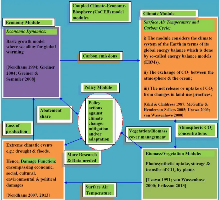
The study is outlined in Figure 2 below. It summarizes the various modules of the study. The next Section, Chapter 2, looks at the literature review.
8
9
CHAPTER 2
LITERATURE REVIEW
This chapter reviews some of the literature related to climate change modelling and integrated assessment modelling. Nowadays there are numerous climate change models; they function to predict future changes in climatic conditions and to help formulate mitigation policies. Integrated assessment models are especially useful in these regards, since they can provide insight into the interaction between different sectors of a larger system. The component models of individual sciences (natural or social) cannot do this.
2.1 Climate change and climate variability
Climate change and climate variability are two important characteristics of climate. According to United Nations Framework Convention on Climate Change(UNFCCC 1992), climate change is a
change of climate which is attributed directly or indirectly to any human activity that alters the composition of the global atmosphere and which is in addition to natural variability observed over comparable time periods. On the other hand, climate variability is the departure from normal or the difference in magnitude between climatic episodes.
The history of scientific study of climate change is long. More than a century ago, for example, Fourier (1824, 1888) was the first to notice that the Earth is a greenhouse, kept warm by an atmosphere that reduces the loss of infrared radiation. The overriding importance of water vapor as a greenhouse gas was recognized even then. In the late 1890s,Arrhenius (1896) was the first to quantitatively relate the concentration of CO2 in the atmosphere to global surface
temperature. Given this long-standing history, one might lament the fact that - perhaps owing, in part, to the politically-charged nature of the topic – many people mistakenly assume that the
10
science that underlies our current understanding of climatic change is, in some way, suspect or unreliable. Of course, the nature of the greenhouse debate is far too complex and multifaceted to lend itself well to simplistic “is it happening or isn’t it?” characterizations.
The vast evidence that the climate of the Earth is changing due to the anthropogenic increase in greenhouse gases (GHGs) is compiled in the successive reports of the Intergovernmental Panel on Climate Change (IPCC 1996a, 2001a, 2007a, 2013), CO2 being the
largest contributor (Farmer and Cook 2013, p. 4; Stern 2008; Stott et al. 2000). Typically, the effect of global warming on the economic system is modeled using integrated assessment models (IAMs). IAMs are motivated by the need to balance the dynamics of carbon accumulation in the atmosphere and the dynamics of de-carbonization of the economy (Nordhaus 1994a). A specific goal of these studies is to evaluate different abatement scenarios as to economic welfare and their effects on GHG emissions.
2.2 Integrated assessment modelling (IAM)
2.2.1 The emergence of IAMs as a science-policy interface
With the immense enhancement in computer technology, integrated modelling surfaced in the mid-1980s as a new paradigm for interfacing science and policy concerning complex environmental issues such as climate change. In the second half of the eighties, it was believed that integrated modelling would be the optimal way to interface science with policy. According to Parson (1994): “To make rational, informed social decisions on such complex, long-term, uncertain issues as global climate change, the capacity to integrate, reconcile, organize, and communicate knowledge across domains to do integrated assessment is essential.” Therefore, integrated assessment models are believed to produce insights that cannot be easily derived from the individual natural or
11
social science component models that have been developed in the past (Weyant 1994); see also, Meyers (2012, pp. 5399 5428) and Rasch (2012, Ch. 8) for a further discussion.
According to Beltran et al. (2005, p. 70), Integrated Assessment (IA) can be defined as an interdisciplinary process of combining, interpreting and communicating knowledge from diverse scientific disciplines in such a way that the whole cause-effect chain of a problem can be evaluated from a synoptic perspective with two characteristics: (i) it should have added value compared to single disciplinary assessment; and (ii) it should provide useful information to decision makers.
2.2.2 Classification of IAMs
Nowadays IAMs are capable of reflecting a range of modelling approaches that aim to provide policy-‐relevant information, and most can be summarized by: (i) policy optimization that seeks optimal policies and (ii) policy evaluation models that assess specific policy measures. The complexity of optimization models is limited, however, because of the requirement of a large number of numerical algorithms in optimization. Therefore these models tend to be based on compact representations of both the socioeconomic and natural science systems. They thus contain a relatively small number of equations, with a limited number of geographic regions. Apart from policy optimization, policy evaluation models tend to be descriptive and can contain much greater modelling detail on bio-geo-physical, economic or social aspects. These models are often referred to as simulation models, and are designed to calculate the consequences of specific climate policy strategies in terms of a suite of environmental, economic, and social performance measures. An early example of this type of model is the Integrated Model to Assess the Global Environment (IMAGE) (Rotmans 1990; Alcamo et al. 1998).
Other policy evaluation models include Asian-Pacific Integrated Model (AIM), Model for Energy Supply Strategy Alternatives and their General Environmental impacts (MESSAGE)
12
(Gusti et al., 2008), etc. These models are not subject to the constraints of optimization models, and therefore can incorporate greater complexity in their representations of natural and social processes at the regional scale without losing detail. Thus, they are generally applied to comparisons of the consequences (e.g., regional economic and environmental impacts) of alternative emissions scenarios. But even with these detailed descriptive capabilities, they are not appropriate to optimize the economic activities of the energy-economy sector.
2.2.3 Application of integrated assessment models
Integrated Assessment Modelling is usually comprehensive, but it produces less detailed models than conventional climate- or socio-economic-centred approaches. It is based on an understanding that feedbacks and interconnections in the climate-society-biosphere system drive its evolution over time (Davies and Simonovic 2008). Rotmans et al. (1997, p. 36) state that integrated assessments “are meant to frame issues and provide a context for debate. They analyze problems from a broad, synoptic perspective.”
Integrated assessment modelling is not a new concept; it rather has a long history of being applied to many problems. Over the past decade or so, integrated assessment models (IAMs) have been widely utilized to analyze the interactions between human activities and the global climate (Weyant et al. 1996). The first IPCC report referenced two IAMs, the Atmospheric Stabilization Framework from US Environmental Protection Agency (EPA) and the Integrated Model for the Assessment of the Global Environment (IMAGE) model from the Netherlands (van Vuuren et al. 2006a). These were employed to assess the factors controlling the emissions and concentrations of GHGs over the next century. Model for the Assessment of Greenhouse-gas Induced Climate Change (MAGICC) was then developed to account ocean heat transport and a carbon cycle component to respond the land-use change; it is a multi-box energy balance model (Meinshausen
13
et al. 2008). Later, MAGICC modelling framework became a foundation for the IPCC process, as it can easily show the climate implications of different emissions scenarios and can be benchmarked to have climate responses that mimics those of any of the GCMs.
Rotmans et al. (1997), mention that the integrated assessment approach allows for an exploration of the interactions and feedbacks between subsystems and provides flexible and fast simulation tools. It also identifies and ranks major uncertainties, and supplies tools for communication between scientists, the public, and policy makers. Davies (2007) provides some examples of integrated assessment models including the Integrated Model to Assess the Greenhouse Effect, IMAGE 2.0 (Alcamo et al. 1994), the Asian Pacific Integrated Model, AIM (Matsuoka et al. 1995), the Model for Evaluating Regional and Global Effects of GHG reduction policies, MERGE (Manne et al. 1995), the Tool to Assess Regional and Global Environmental and health Targets for Sustainability, TARGETS (Rotmans and de Vries 1997), the Integrated Global System Model, IGSM (Prinn et al. 1999), Integrated Climate Assessment Model, ICAM (Dowlatabadi 2000), the Dynamics Integrated Climate-Economy model, DICE (Nordhaus and Boyer 2000), the Feedback-Rich Energy-Economy model, FREE (Fiddaman 1997; Fiddaman 2002), and World3(Meadows et al. 2004). The list of IAMs and Computable General Equilibrium (CGE) models used in climate policy analyses is long. The reader can refer to Ortiz and Markandya (2009) and Stanton et al. (2008) for a literature review of some of these models.
Most IAMs consist of (i) an economy module in which the interactions among economic sectors and agents are represented; (ii) a climate module representing the relationships between GHG emissions and concentrations and temperature changes; and (iii) predetermined relationships between both modules; i.e. damage functions representing the impact of temperature changes in the economy, and abatement cost functions summarizing the available climate change mitigation
14
options. The level of details employed in each of these components characterizes and differentiates the existing models (Ortiz et al. 2011).
It has been predicted that global climate change will have significant impacts on society and the economy, and that the adaptation measures to tackle global climate change will be accompanied with very large economic burden. It is estimated that GHG emissions will increase to over one-half of total global emissions by the end of the next century (Akhtar 2011, p. 42). The Integrated Assessment Model (IAM) provides a convenient framework for combining knowledge from a wide range of disciplines; it is one of the most effective tools to increase the interaction among these groups.
2.2.4 Challenges for IAM studies
The foremost challenge for IAM Studies is the integration of the natural and socioeconomic systems in order to better model the relationship between human activities and the global environment. To the present, many integrated assessment models share the same basic framework. Whether current IAMs have reached a level of development where they can serve as the adequate basis for judgments in formulating actual global environmental measures is debatable. Modellers appear to agree, however, that for the most part the framework itself is acceptable. The integrated assessment of global environmental issues from the perspectives of the natural and social sciences is not a field of learning involving the pursuit of truth. Rather, it is a practical science that aims at providing useful guidance to policy makers seeking to establish rules and policies that help smooth the relationships between natural rule, the global environment and humanity. Conventionally, it is possible to encapsulate the relationships between such practical scientific studies and the real world in a relatively simple framework.
15
Any attempt to represent fully a complex issue and its numerous interlinkages with other issues in a quantitative modelling framework is doomed to failure (Rotmans and van Asselt 2001). However, even a simplified integrated assessment model can provide valuable insight into certain aspects of complex issues. Through their intersectoral links and communication facilities, IAMs can provide more accurate representations of such problems as climate change than those studies based on a conventional modelling framework. IAMs thus remain a very useful tool for decision makers, scientists– especially in the field of climate change studies.
In analyzing implications of climate policies, these models often assume that the growth rate of the economy is exogenously given, and feedback effects of lower GHGs concentrations in the atmosphere on economic growth are frequently neglected. For example, in Nordhaus and Boyer (2000) different abatement scenarios are analyzed where the growth rate of the economy is assumed to be an exogenous variable and the results are compared with the social optimum. Also, the fundamental alterations in wealth holdings are systematically downplayed by the practices of current integrated assessment modeling (Decanio 2003; Kirman 1992, p. 132).
2.2.5 Improvements of IAMs
There are several aspects in which IAMs need to be improved. Besides the need for better data on expected economic damages of climate change, future research on IAMs should consider:
! Economic modeling in developing countries. Most current IAMs do not match the economic and social organization of developing countries well (Carraro 2002). This leads to biases in global assessments where climate change mitigation and impacts are evaluated in developing countries as if their economies work like those of developed countries.
! Endogenous Technical Change. Most IAMs models have considered technical change as an
16
historical records (Kelly and Kolstad 1999). But, technical change might be critically important in GHGs mitigation scenarios. For example, the development of inexpensive electric automobiles or solar power might reduce significantly GHGs emissions at low cost. Further research is needed in order to incorporate endogenous innovation in climate models.
! Specifying Regulation Instruments (Kelly and Kolstad 1999). Most IAMs calculate optimal
carbon taxes for achieving emission reduction targets. But, the impact of recycling such tax revenues needs to be evaluated. Also, regulation instruments have associated monitoring costs and penalties for non-compliance which would reduce the overall efficiency of mitigation strategies.
! Adjustment to Climate Change (Kelly and Kolstad 1999). Agents within the economy would
respond to global warming in order to reduce its impacts. For example, given changes in rainfall and precipitation, farmers could modify crop choice in order to reduce the losses caused by climate change. Also, migration patterns and urbanization in developing countries might be modified in such a way that areas highly vulnerable to climate change would limit their growth.
! Include carbon mitigation in sinks. One of the major drawbacks of IAMs is that they mainly
focus on mitigation in the energy sector (van Vuuren et al. 2006b, p. 166). For example, the RICE (Regional Dynamic Integrated model of Climate and the Economy) and DICE (Dynamic Integrated model of Climate and the Economy) (Nordhaus and Boyer 2000) models consider emissions from land use asexogenous (see also, Tol 2010 p. 97). But, GHGs emissions from land use and current terrestrial uptake are significant, so including GHGs mitigation in sinks is something to be considered within IAMs (Wise et al. 2009).
17
2.2.6 This study
This thesis looks at the interaction between global warming and economic growth, along the lines of the Dynamic Integrated model of Climate and the Economy (DICE) of Nordhaus (1994a), with subsequent updates in Nordhaus and Boyer (2000), Nordhaus (2007, 2008, 2010, and 2013a). Greiner (2004) (see also Greiner and Semmler 2008) extended the DICE framework by including endogenous growth, to account for the fact that environmental policy affects not only the level of economic variables but also the long-run growth rate. Using the extended DICE model, Greiner argues that higher abatement activities reduce GHG emissions and may lead to a rise or decline in growth. The net effect on growth depends on the specification of the function between the economic damage and climate change.
Since anthropogenic GHGsare the result of economic activities, the main shortcoming in Greiner’s (2004) approach is that of treating industrial CO2 emissions as constant over time.
Another problematic aspect of Greiner’s emissions formulation is its inability to allow for zero abatement activities. In fact, his formulation only holds for a minimum level of abatement.
This study addresses these issues by using a novel approach to formulating emissions that depend on economic growth and vary over time; in this approach, abatement equal to zero corresponds to Business As Usual (BAU). To do so, this work uses logistic functions (Akaev 2012; Sahal 1981) that yield the global dynamics of carbon intensity, i.e. of energy emissions per unit of energy consumed, and of energy intensity, i.e. of energy use per unit of aggregate gross domestic product (GDP) throughout the whole 21st century (Akaev 2012).
The study further uses the extended DICE modeling framework by considering both human and physical capital accumulation, in addition to the GHG emissions, as well as a ratio of abatement spending to the tax revenue or abatement share (see also, Greiner 2004; Greiner and Semmler 2008). The methodology utilized can analytically clarify the mutual causality between
18
economic growth and the climate change–related damages and show how to alter this relationship by the use of various mitigation measures geared toward reduction of CO2 emissions (Hannart et
al. 2013; Metz et al. 2007). The study will use the abatement share to invest in the increase of overall energy efficiency of the economy (Diesendorf 2014, p. 143) and decrease of overall carbon intensity of the energy system. It will be shown below that over the next few decades, up to the mid-21st century, mitigation costs do hinder economic growth, but that this growth reduction is compensated later on by the having avoided negative impacts of climate change on the economy; see also Kovalevsky and Hasselmann (2014, Figure 2).
The thesis also introduces CO2 capturing and storing (CCS) technologies and reduction of
deforestation, as well as increasing photosynthetic biomass sinks as a method of controlling atmospheric CO2 and consequently the intensity and frequency of climate change related damages.
This move is necessitated on one part by the fact that most of the scenario studies that aim to identify and evaluate climate change mitigation strategies (see, e.g., Hourcade and Shukla 2001; Morita and Robinson 2001) focus on the energy sector (van Vuuren et al. 2006b, p. 166). Examples of studies that focus on the energy sector are the RICE (Regional Dynamic Integrated model of Climate and the Economy) and DICE (Dynamic Integrated model of Climate and the Economy) (Nordhaus and Boyer 2000) models which consider emissions from land-use as exogenous (see also, Tol 2010 p. 97). Nevertheless, GHG emissions from deforestation and current terrestrial uptake are significant, so including GHG mitigation in the biota sinks has to be considered within integrated assessment models (IAMs), cf. Wise et al. (2009).
Several studies provide evidence that forest carbon sequestration can reduce atmospheric CO2 concentration significantly and could be a cost-efficient way for curbing climate change (e.g.,
Bosetti et al. 2011; Gullison et al. 2007; Tavoni et al. 2007; Wise et al. 2009). Again, most earlier studies have not considered the more recent mitigation options currently being discussed in the
19
context of ambitious emission reduction, such as hydrogen and carbon capture and storage (CCS); see Edmonds et al. (2004), IEA (2004) and IPCC (2005). Given current insights into climate risks and the state of the mitigation literature, then, there is a very understandable and explicit need for comprehensive scenarios that explore different long-term strategies to stabilize GHG emissions at low levels (Metz and van Vuuren 2006; Morita et al. 2001). This study works towards this direction by studying relevant economic aspects of deforestation control and carbon sequestration in forests, as well as the widespread application of CCS technologies as alternative policy measures for climate change mitigation.
The Coupled Climate-Economy-Biosphere (CoCEB) model is not intended to give a detailed quantitative description of all the processes involved, nor to make specific predictions for the latter part of this century. It is a reduced-complexity model that attempts to incorporate the climate-economy-biosphere interactions and feedbacks, while using the smallest number of variables and equations needed to capture the main mechanisms involved in the evolution of the coupled system. We merely wish to trade greater detail for more flexibility in the analysis of the dynamical interactions between the different variables. The modeling framework here brings together and summarizes information from diverse fields in the literature on climate change mitigation measures and their associated costs, and allows comparing them in a coherent way. The need for a hierarchy of models of increasing complexity is an idea that dates back in the climate sciences to the beginnings of numerical modeling (e.g., Schneider and Dickinson 1974), and has been broadly developed and applied since (Ghil 2001, and references therein).
The study seeks to show that:
(i) Investment in low-carbon technologies helps to reduce the volume of industrial CO2
emissions, lower temperature deviations, and lead to positive effects in economic growth.
20
(ii) Low investment in CCS contributes to reducing industrial carbon emissions and to increasing GDP growth, but further investment leads to a smaller reduction in emissions, as well as in the incremental GDP growth.
(iii) Enhanced deforestation control contributes to a reduction in both deforestation emissions and atmospheric CO2 concentration, thus reducing the impacts of climate change and
contributing to a slight appreciation of GDP growth, but this effect is very small compared to that of implementing low carbon technologies or CCS.
(iv) The result in (ii) is very sensitive to the formulation of CCS costs. To the contrary, the results for deforestation control are less sensitive to the formulation of its cost.
A large range of hypotheses on CCS costs appears in the literature, and our modeling framework permits to span this range and check the sensitivity of results.
The sensitivity study carried out is not intended to make precise calibrations; rather, the study wants to provide adiagnostic tool for studying qualitatively how various climate policies affect the economy.
The next chapter describes the theoretical model, detailing the additions with respect to Nordhaus (2013a), Greiner (2004) and Greiner and Semmler (2008), introduces the biomass equation and the effect on the carbon emissions of CCS and of deforestation control. Chapter 4 presents the numerical simulations and their results. In Chapter 5, we test the sensitivity of the results to key parameters. Chapter 6 summarizes, discusses the results, and formulates our conclusions with caveats and avenues for future research.
21
CHAPTER 3
MODEL DESCRIPTION
3.1 Climate module
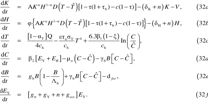
The time evolution of the average surface temperature T (SAT) on Earth is modeled via an energy balance equation given by
(
T)
T a 4 1(
)
h h h 1 α Q εσ τ 6.3β 1 ξ d In ˆ d 4 T C T t c c c C − − ⎛ ⎞ = − + ⎜ ⎟ ⎝ ⎠, (1) see, for instance, Ghil and Childress (1987, Ch. 10), Hans and Hans (2013, Ch. 2) or McGuffie and Henderson-Sellers (2005, p. 81–85; 2014). Here the first and second terms on the right-hand side are incoming and outgoing radiative fluxes respectively, while the third term is radiative forcing due to increase in GHGs (Greiner and Semmler 2008; Kemfert 2002); σ is the Stefan-Boltzmann T constant, τ the infrared (long-wave) transmissivity of the atmosphere, ε the emissivity that gives a the ratio of actual emission to blackbody emission, α the mean planetary albedo, Q is the T average solar constant. The specific heat capacity c of Earth is largely determined by the oceans h(Levitus et al. 2005) and it is taken equal to 16.7 Wm–2K-1 (Schwartz 2007, 2008), which corresponds to an ocean fractional area of 0.71 and a depth of 150 m of the ocean mixed layer. The current CO2 concentration C is given in gigatons of carbon (GtC, 1 Gt = 1015 grams) and ˆC
is the pre-industrial CO2 concentration. All the feedbacks, are represented in this highly idealized
model by the factor β , which is assumed to take values between 1.1 and 3.4 (Greiner and 1 Semmler 2008, p. 62); in this study, it was assumed that β1 =3.3. The parameter ξ 0.23= captures the fact that part of the warmth generated by the greenhouse effect is absorbed by the oceans and
22
transported from their upper layers to the deep sea (Greiner and Semmler 2008). The other parameters have standard values that are listed in Table 1.
At equilibrium, that is for dT dt=0, Equation (1) gives an average SAT of 14 0C for the pre-industrial GHG concentration, i.e. for C=Cˆ. Doubling the CO2 concentration in Equation (1)
yields an increase of about 3.3 0C in equilibrium temperature, to 17 0C. This increase lies within the range of IPCC estimates, between 1.5 and 4.5 0C (Charney et al. 1979; IPCC 2001a, p. 67; IPCC 2013) with a best estimate of about 3.0 0C (IPCC 2007a, p.12).
The study represents the evolution C of the concentration of CO2 in the atmosphere,
following Uzawa (2003) and Greiner and Semmler (2008), as
(
)
2 Y o ˆ β µ dC E C C dt = − − , (2)where E is industrial COY 2 emissions. The excess C above pre-industrial level is reduced by the
combined effect of land and ocean sinks. The inverse µ of the atmospheric lifetime of COo 2 is
estimated in the literature to lie within an uncertainty range that spans 0.005 0.2 (IPCC 2001a, p. 38); The study takes it here to equal µo =1 120=0.0083, i.e. closer to the lower end of the range (IPCC 2001a, p. 38; Nordhaus 1994a, p. 21). The fact that a certain part of GHG emissions is taken up by the oceans and does not remain in the atmosphere is reflected in Equation (2) by the parameter β . 2
3.2 Economy module
In Greiner (2004) and Greiner and Semmler (2008) the per capita GDP, Y, is given by a modified version of a constant-return-to scale Cobb-Douglas production function (Cobb and Douglas 1928),
( )
α 1 α ˆ A23
Here K is the per capita physical capital, H is the per capita human capital, A>0 the total factor of productivity, 0< <α 1 is the capital share, D T
( )
− is the damage, expressed as a function of Tˆthe temperature difference due to climate change. The damage function is described in Subsection (3.3.3) below.
The economy income identity in per capita variables is given by E E
Y −X = +I M +G , (4) with X =τY the (per capita) tax revenue, 0< <τ 1 the per annum tax rate, I investment, M E
consumption, and G abatement activities. This means that national income after tax is used for E
investment, consumption, and abatement. The study assumes that G is expressed as a fraction of E
X ,
E τb τ τb
G = X = Y, (5) with 0≤τb <1 the ratio of per annum abatement share, used as a policy tool. Consumption is also expressed as a fraction of Y after tax, that is,
( )
E 1 τM =c − Y, (6) with 0< <c 1 the global annual consumption share.
The accumulation of per capita physical capital K is assumed to obey
(
)
E E K d δ d K Y X M G n K t = − − − − + , (7)the logistic-type human population growth rate 0< <n 1 is given, in turn, by
n d 1 1 d 1 δ n n t ⎛ ⎞ =⎜ − ⎟ − ⎝ ⎠ , (8) with δ being the per year decline rate of n , and n δ the per year depreciation rate of physical K capital. Substituting the definitions of Y, X , M , and E G into Equation (7) the study gets E