MIT Joint Program on the
Science and Policy of Global Change
A Coupled Atmosphere-Ocean Model of
Intermediate Complexity for Climate Change Study
Igor V. Kamenkovich, Andrei P. Sokolov and Peter H. Stone
Report No. 60
The MIT Joint Program on the Science and Policy of Global Change is an organization for research,
independent policy analysis, and public education in global environmental change. It seeks to provide leadership in understanding scientific, economic, and ecological aspects of this difficult issue, and combining them into policy assessments that serve the needs of ongoing national and international discussions. To this end, the Program brings together an interdisciplinary group from two established research centers at MIT: the Center for Global Change Science (CGCS) and the Center for Energy and Environmental Policy Research (CEEPR). These two centers bridge many key areas of the needed intellectual work, and additional essential areas are covered by other MIT departments, by collaboration with the Ecosystems Center of the Marine Biology Laboratory (MBL) at Woods Hole, and by short- and long-term visitors to the Program. The Program involves sponsorship and active participation by industry, government, and non-profit organizations.
To inform processes of policy development and implementation, climate change research needs to focus on improving the prediction of those variables that are most relevant to economic, social, and environmental effects. In turn, the greenhouse gas and atmospheric aerosol assumptions underlying climate analysis need to be related to the economic, technological, and political forces that drive emissions, and to the results of international agreements and mitigation. Further, assessments of possible societal and ecosystem impacts, and analysis of mitigation strategies, need to be based on realistic evaluation of the uncertainties of climate science.
This report is one of a series intended to communicate research results and improve public understanding of climate issues, thereby contributing to informed debate about the climate issue, the uncertainties, and the economic and social implications of policy alternatives. Titles in the Report Series to date are listed on the inside back cover.
Henry D. Jacoby and Ronald G. Prinn,
Program Co-Directors
For more information, contact the Program office:
MIT Joint Program on the Science and Policy of Global Change
Postal Address: 77 Massachusetts Avenue
MIT E40-271
Cambridge, MA 02139-4307 (USA)
Location: One Amherst Street, Cambridge
Building E40, Room 271
Massachusetts Institute of Technology
Access: Telephone: (617) 253-7492
Fax: (617) 253-9845
E-mail: [email protected]
Web site: http://web.mit.edu/globalchange/
A Coupled Atmosphere-Ocean Model of Intermediate Complexity
for Climate Change Study
*Igor V. Kamenkovich1, Andrei Sokolov2 and Peter H. Stone2 Abstract
A three-dimensional ocean model with an idealized global geometry and coarse resolution coupled to a two-dimensional (zonal-mean) statistical-dynamical atmospheric model is used to investigate the response to the increasing CO2 concentration in the atmosphere. Long-term present-day climate simulations with and
without asynchronous integration in the ocean have been carried out with and without flux adjustments, and with either the Gent-McWilliams (GM) parameterization scheme or horizontal diffusion (HD). The results show that a moderate degree of asynchronous coupling between the oceans momentum and tracer fields still allows an accurate simulation of transient behavior, including the seasonal cycle. The use of the GM scheme significantly weakens the Deacon Cell and eliminates convection in the Southern Ocean. The deep ocean temperatures systematically decrease in the runs without flux adjustment. We demonstrate that the mismatch between heat transports in the uncoupled states of two models is the main cause for the systematic drift.
The global warming experiments are sensitive to the parameterization of the sub-grid mixing. The penetration of anomalous heat in the Southern Ocean is noticeably weaker in the case with the GM scheme. As a result, the transient surface response exhibits less inter-hemispheric asymmetry than in the HD case. The equilibrium surface warming of the Southern Hemisphere is noticeably larger than that of the Northern Hemisphere in the GM case; the equilibrium warming is more uniform in the HD case. Use of the GM parameterization also leads to smaller decrease and faster recovery of the sinking in the North Atlantic. The increase in the surface heat fluxes is shown to be the dominant factor causing the weakening of the circulation. Results of the simulation with different rates of increase in the forcing are also presented.
Contents
1. Introduction ... 2
2. Description of the Model ... 3
2.1 Ocean Component ... 3
2.2 Atmospheric Component... 5
2.3 Coupling Procedure ... 6
2.4 Asynchronous Integration ... 7
3. Present-day Climate Simulations... 8
3.1 Anomaly Coupling: Experiments ANHD and ANGM ... 8
3.2 Direct Coupling: Causes for the Climate Drift. Experiments DIRGHD and DIRGM ... 10
3.2.1 Surface Response ... 10
3.2.2 Deep Temperature Drift. Experiments DIRGMN and FWFGM... 11
4. Global Change Experiments... 14
4.1 Response to CO2 Increase Dependence on Parameterization of Sub-grid Scale Mixing ... 16
4.1.1 Temperature Response ... 16
4.1.2 Changes in the Circulation... 20
4.2 Dependence of Model Response on the Rate of the CO2 Increase... 22
5. Summary and Conclusions ... 23
References ... 26
* Institute for the Study of Atmosphere and Ocean, University of Washington, Contribution Number 761 1
Corresponding author: Joint Institute for the Study of the Atmosphere and the Oceans, Department of Atmospheric Sciences, Box 354235, University of Washington, Seattle, WA 98195-4235
2
1. INTRODUCTION
Climate change simulations with coupled atmosphere-ocean models have shown that the oceans play an important role in defining both transient and equilibrium responses of the climate system to changes in greenhouse gases (GHGs) and aerosols concentrations in the atmosphere. There are, however, significant uncertainties in oceanic response to an external forcing. The rate of heat uptake by the deep ocean differs from one ocean model to another (IPCC, 1996; Murphy and Mitchell, 1995; Sokolov and Stone, 1998). The magnitude of weakening of the thermohaline circulation, which can lead to fundamental changes in the state of climate system, is also rather different between simulations with different ocean models. In addition, there is a significant uncertainty in the rate of the future increase in concentrations of GHGs and aerosols, while it was shown that changes in ocean circulation strongly depend on this rate (Schmittner and Stocker, 1999; Stouffer and Manabe, 1999).
Therefore, a systematic study of possible climate changes requires carrying out a significant number of long-term simulations, which in turn requires the use of computationally efficient models. A number of coupled atmosphere-ocean models of intermediate complexity have been developed in recent years (Stoker, 1992; Petuchov et al., 1999; Wiebe and Weaver, 1999). In this paper we document a model, which consists of an ocean model with simplified geometry coupled to a two-dimensional atmospheric model (Sokolov and Stone, 1998). The atmospheric component of the model was developed from the GISS general circulation model (GCM) (Hansen et al., 1983). It solves the primitive equations as an initial value problem and includes parameterizations for all the main physical processes. Therefore it can simulate atmospheric circulation and its response to external forcing in a more realistic way then the energy-balance models typically used in coupled models of intermediate complexity. At the same time, it is efficient enough computationally to be used in climate change studies that require carrying out multiple long-term climate simulations (Prinn et al., 1999).
In most of the existing coupled atmosphere ocean general circulation models (AOGCMs) fluxes of heat, moisture and momentum through the atmosphere-ocean interface have to be adjusted to prevent drift of the climate system into an unrealistic state. Some of the recently developed most sophisticated atmosphere-ocean coupled models (Boville and Gent, 1998; Gordon et al., 2000) are stable for multi-century integrations without such an adjustment.
Systematic drift in temperature in the upper ocean in those models is significantly smaller than in the older generations of models (Manabe and Stouffer, 1988). However, large drift in the salinity and deep-ocean temperature is still present even in those models (Boville and Gent, 1998; Bryan, 1998; Gordon et al., 2000). Taking into account the crude spatial resolution and other
simplifications made in both models components, it is not surprising that the use of flux adjustment is required in simulations with the model described here. To find the main factors causing climate drift in our model we also performed a number of simulations without or with a partial flux adjustment.
Parameterization of the effects of mesoscale oceanic eddies in the coarse-resolution numerical models remains a challenging problem for the modeling community. The oldest and still the
most widely used approach is to use a horizontal diffusion (HD) with constant coefficients. The more recent Gent-McWilliams scheme (Gent and McWilliams, 1991; GM hereafter) is generally believed to improve simulated ocean circulation. Jiang et al. (1999) show that the North Atlantic (NA) sinking rates are overestimated in their model with realistic mixed boundary conditions if the HD scheme is used. The application of the GM scheme, in contrast, results in more realistic rates of deep-water formation in that region. Large differences between the two schemes are also observed in the Southern Oceans, where the GM scheme reduces deep convection and
significantly weakens the Deacon Cell, which is considered to be too strong in many simulations with HD (Boning et al., 1995; Danabasoglu and McWilliams, 1995; McDougall et al., 1996).
The differences in circulation and reduction of diapycnal mixing, in turn, affect the vertical distribution of tracers. McDougall et al. (1996) report significant improvements in deep density fields as a result of using the GM scheme. They suggest that HD results in unrealistically deep mixed layers in the Southern Ocean. Results of recent simulations with ocean GCMs (IPCC, 1996) support this conclusion by showing that the distribution of CFC11 agrees better with observations when the GM scheme is used. These results suggest that the HD scheme
overestimates the efficiency of the heat uptake in the Southern Ocean in the HD case (see also Hirst et al., 1996; Mitchell et al., 1998; Wiebe and Weaver, 1999). An overestimated rate at which heat penetrates into the deep ocean should generally result in an underestimation of surface warming in response to anomalous atmospheric heating.
The standard version of our model incorporates the GM scheme. At the same time both present-day climate and climate change simulations with HD were also carried out. We describe the models components and coupling procedure in Section 2. We describe present-day climate simulations in Section 3, where we also analyze the origins of systematic drift in temperature in the model with no flux adjustment. We test the dependence of the model response to increasing CO2 in the atmosphere on the parameterization of mesoscale eddies in Section 4. We concentrate on the surface warming, distribution of anomalous heating with depth and stability of the
thermohaline circulation. Since the effects of the use of flux adjustment on a models predictions remain unclear (Marotzke and Stone, 1995; Fanning and Weaver, 1997), we also compare responses in the models with and without flux adjustment. The summary and conclusions are presented in Section 5.
2.DESCRIPTION OF THE MODEL
The model consists of atmosphere and ocean components. Each component was spun up independently prior to coupling using the observed surface fluxes and surface temperature.
2.1 Ocean Component
The ocean component of the coupled model is the MOM2 model (Pacanowski et al., 1996) with idealized geometry. It consists of two rectangular basins (Figure 1): Pacific extending from 48ßS to 60ßN, and Atlantic extending from 48ßS to 72ßN. The basins are connected by a channel (Atlantic circumpolar current, ACC), which extends from 48ßS to 64ßS. The model
Drake Passage (between Pacific and Atlantic) extends only from 52ßS to 64ßS. The Pacific basin is 120ß wide and Atlantic basin is 60ßwide. Coupling of this model with a zonal-mean atmosphere model justifies the use of the idealized geometry in our study.
The resolution in latitude is 4ß; resolution in longitude varies from 1ß near the meridional solid boundaries to 3.75ß in the interior. Better resolution of the boundary currents has been shown to improve the simulated
0 50 100 150 -60 -40 -20 0 20 40 60 Longitude Latitude Sill, 2900 m deep 48ßS 72ßN 64ßS Current (ACC) Pacific Basin Basin 120ß wide 60ß wide Atlantic Antarctic Circumpolar
Figure 1. Geometry of the ocean model.
meridional heat transport in an ocean GCM (Kamenkovich et al., 2000). The model has 15 layers in the vertical with thicknesses increasing downward from 50 to 500 m. The ocean is 4,500 m deep and the bottom is flat everywhere except in the Drake Passage, where there is a sill 2,900 m deep.
No-slip conditions for horizontal velocity are applied at the lateral walls. Free-slip conditions are used at the bottom, except in the ACC, where a bottom drag is applied. Boundary conditions for tracers are insulating at lateral walls and bottom. We employ either the GM or HD schemes for the parameterization of eddy transports of tracers. Mixing coefficients are 5 x 10⁴
and 0.01 m2/sec for horizontal and vertical momentum viscosity, and 103 and 5 x 10—5 m2/sec for horizontal and vertical tracer diffusivity. In the GM case, isopycnal diffusivity and isopycnal thickness diffusivity are 103
m2
/sec each with no background horizontal diffusion.
The surface boundary conditions used to spin-up the ocean model are taken from Jiang et al. (1999), who constructed the datasets using the data sources listed below; see their study for a complete description of the datasets. The heat flux consists of two terms:
1 ) ( d T T C H F obs obs H ρ λ − + = [1]
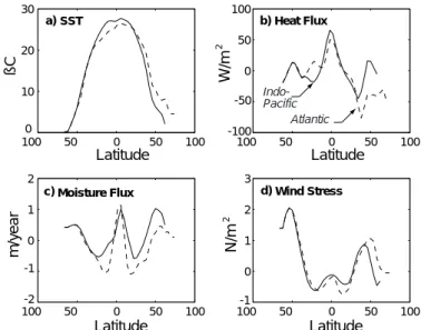
The first term is the observed heat flux from dataset TS97 (Trenberth, 1998) an improved version of Trenberth and Solomon (1994). The second term on the right-hand side of Eq. 1 represents relaxation of model sea surface temperature (SST; T) to the observed SST (Tobs; from Levitus and Boyer, 1994). Restoring time scale λ is 60 days, d1 is the thickness of the upper layer (52 meters), C is the specific heat capacity, and ρ is the density of the water. Note that long-term average of this relaxation term would be zero if the model reproduced observed temperature when forced by observed fluxes. The moisture flux is specified and is based on P-E data from Schmitt et al. (1989), river runoff data from Perry et al. (1996) and ice-calving data from Reeh (1994). Wind stress is taken from Trenberth (1989).
We took basin zonal means of all observed quantities in the boundary conditions (data from Indo-Pacific are used for the models Pacific). Heat and moisture fluxes are re-balanced to ensure zero net flux through the ocean surface. The results are shown in Figure 2. The SST, heat fluxes, and wind stress have a seasonal cycle, while freshwater flux is an annual mean.
A thermodynamic ice model is used for representing sea ice. The model has two layers and computes ice concentration (the percentage of area covered by ice) and ice thickness. The model is used in all experiments except one (DIRGMN), in which no ice formation is allowed.
We obtain two different equilibrium
100 50 0 50 100 0 10 20 30 SST Latitude ßC 100 50 0 50 100 -100 -50 0 50 100 Heat Flux Latitude W/m 2 100 50 0 50 100 -2 -1 0 1 2 Moisture Flux Latitude m/y ear 100-1 50 0 50 100 0 1 2 3 Wind Stress Latitude N/m 2 Atlantic Indo-Pacific a) b) c) d)
Figure 2. Surface boundary conditions used for the
spin-up of the ocean component: Indo-Pacific basin (solid line) and Atlantic (dashed line).
(a) Sea surface temperature (˚C); (b) Heat flux into
the ocean (W/m2); (c) Moisture flux into the ocean
(m/yr); (d) Wind stress (N/m2).
states, one with the use of GM and another with HD, which are in reasonable agreement with the observed climate. The circulation has the form of a conveyor belt with water sinking in the North Atlantic and upwelling in the South Atlantic and Pacific oceans. SST is within 1.5ßC of the observed values.
2.2 Atmospheric Component
The two-dimensional (zonally averaged) statistical-dynamical atmospheric model used in this study (Sokolov and Stone, 1998) was developed on the basis of the GISS GCM (Hansen et al., 1983). The model solves the primitive equations in latitude-pressure coordinates. The models grid contains 24 points in latitude, corresponding to a resolution of 7.826ß, and 9 layers in the vertical. The models numerics and most of the parameterizations of physical processes
(radiation, convection, etc.) are closely parallel to those of the GISS GCM. The model also includes parameterizations of heat, moisture, and momentum transports by large-scale eddies (Stone and Yao, 1987, 1990). In contrast with energy-balance models used as an atmospheric component in many coupled models of intermediate complexity (e.g., Stocker and Shmittner, 1997; Wiebe and Weaver, 1999), the MIT two-dimensional (2D) model has complete moisture and momentum cycles and reproduces most of the non-linear interactions and feedbacks simulated by atmospheric GCMs.
The 2D model, as well as the GISS GCM, allows up to four different kinds of surfaces in the same grid cell, namely open ocean, sea-ice, land, and land-ice. The surface characteristics as well as turbulent and radiative fluxes are calculated separately for each kind of surface while the
atmosphere above is assumed to be well mixed horizontally. The atmospheric model uses a realistic land/ocean ratio for each latitude belt.
As was shown by Sokolov and Stone (1998), the model reproduces the major features of the present-day climate reasonably well. Since the model is to be used for climate change
predictions, it is noteworthy that the seasonal climate variations are also reproduced realistically. The models sensitivity to an external forcing can be varied by changing the strength of cloud feedback (see Hansen et al., 1993; Sokolov and Stone, 1998). The response of the atmospheric model coupled to a mixed layer ocean model to the increase in the atmospheric CO2
concentration shows all the main features found in most GCM simulations. The dependence of different climate variables, such as precipitation, and surface fluxes on surface warming found in simulations with of the 2D model with different sensitivities is similar to that shown by atmospheric GCMs with different sensitivities (Sokolov and Stone, 1998). At the same time, the 2D model is much faster than a 3D GCM with similar latitudinal and vertical resolution.
2.3 Coupling Procedure
Coupling takes place twice a day. The atmospheric model calculates 12-hour means of values of the heat and fresh-water fluxes over open ocean Ho, Fo, their derivatives with respect to SST dHo /dT, dFo /dT, heat flux through the bottom of the ice HI and the wind stress. These quantities are then linearly interpolated to the oceanic grid. Total heat and fresh-water fluxes for the ocean model are: ) 1 )( ( ) 1 ( −γ + γ + − −γ = T T dT dH H H F o i o H [2] ) 1 )( ( ) 1 ( −γ + γ + − −γ = T T dT dF F F F o i o w [3]
where γ is the fractional ice area (concentration) and Fi fresh water flux due to ice melting/ freezing. T is SST at a given ocean point, and the overbar denotes its global zonal mean. The last terms on the right-hand sides of the equations account for the fact that the 2D atmospheric model computes heat and moisture fluxes using zonal mean SST; these terms allow for zonal variations in surface fluxes. The zonal mean of the wind stress is used at a given latitude. The atmospheric component also passes to the ocean model the amount of ice melted from above.
The ocean model, after being integrated twelve hours forced by these fluxes, supplies the atmosphere with a zonal mean of SST, sea ice thickness and its concentration. Values on the atmospheric grid are calculated as area-weighted means of corresponding values on the oceanic grid. Due to the different latitudinal extends of the two models, at the two southernmost and three northernmost points of the atmospheric grid SST is calculated by a mixed layer ocean model. Sea ice characteristics are calculated by a zonally averaged version of the sea ice model described above. In climate change simulations heat mixing into the deep ocean at these points is parameterized by diffusion of the mixed layer temperature deviation from its present-day climate value (Sokolov and Stone, 1998).
We use here two different coupling procedures: with flux adjustment and without it (direct coupling). Flux adjustments in the former method are calculated as differences between the values of heat, moisture and momentum fluxes used to spin-up the ocean model (see Section 2.1) and the corresponding values obtained in the simulation with the atmospheric model forced by observed SST and sea ice. In other words in this mode, hereafter called anomaly coupling, the ocean model is forced by the anomalies in fluxes of the atmospheric model added to the corresponding fluxes used in the ocean-only simulations. The anomalies are identical in both basins. In the anomaly coupling case SST is adjusted by the difference between observed values and those diagnosed from the spin-up steady state of the ocean model. A similar coupling technique is implemented in simulations with the MPI AOGCM by Voss et al. (1998).
2.4 Asynchronous Integration We use an asynchronous integration (Bryan, 1984) with different values of the ratio between time steps for tracer and momentum equations in the ocean model. Three values of this accelerating parameter are tested prior to global-change experiments: unity
(synchronous integration, 1 hour for the tracer and momentum time steps), 12 ( as12 case, 12 hours and 1 hour) and 192 ( as192 case, 2 days and 15 minutes). Annual means of resulting dynamical fields agree well in all three cases. Monthly means of heat transport, however, show significant differences between the synchronous and the as192 cases. In contrast, results in the as12 case are very close to those from the synchronous integration. To illustrate this, we present in Figure 3 the comparison of the monthly means of the meridional heat transports in the Atlantic between as192, as12 and a synchronous run for the anomaly-coupled model with the GM scheme.
100 50 0 50 100 100 50 0 50 100 100 50 0 50 100 100 50 0 50 100 100 50 0 50 100 100 50 0 50 100 -0.5 0 0.5 1 1.5 2 Feb -0.5 0 0.5 1 1.5 Apr -0.2 0 0.2 0.4 0.6 0.8 1 Jun -0.4 -0.2 0 0.2 0.4 0.6 0.8 1 Aug -0.5 0 0.5 1 1.5 Oct -0.5 0 0.5 1 1.5 Dec synch as192 as12 Latitude Latitude W/m 2 W/m 2 W/m 2 W/m 2 W/m 2 W/m 2
Figure 3. Monthly mean meridional heat transports
(in W/m2) in the Atlantic for three different
integration methods: as192 (black line),
as12 (gray line), and synchronous (dashed). The
corresponding month is shown in each panel.
Temporal changes in circulation and temperature fields are both reflected in the values of heat transport. The differences in the Pacific basin are analogous.
We then test the applicability of the as12 technique again in the anomaly-coupled global change experiment with CO2 concentration increasing at the rate of 2% per year. Temporal changes in the circulation and temperature fields in this case are among the largest of all our experiments (see Section 4.3), and this case serves as the most severe test of the asynchronous technique. Nevertheless, even in this case the differences between the results of the as12 and synchronous calculations (not shown) no larger than those shown in Figure 3. Thus in what follows, we will employ asynchronous integration with accelerating factor 12. It allows us to increase the integration speed of the coupled model by a factor of 6.5. As a result, a 100 year coupled run with the ocean model employing the GM scheme takes about 10 hours on a single 500 MHz 21264 CPU of a Compaq AlphaServer DS20, which has SPECfp95 equal to 58.7. 3. PRESENT-DAY CLIMATE SIMULATIONS
Table 1. Present-Day Climate Simulations
Mixing Fluxes Adjusted
Name Scheme heat/SST moisture momentum
ANGM GM yes ANHD HD yes DIRGM GM no DIRGMNa GM no DIRHD HD no WFWGM GM yes no no a
Note: no sea ice
We now discuss the results of our coupled experiments. We base our analysis on annual mean, global zonal average fields. Descriptions of the experiments are given in Table 1.
3.1 Anomaly Coupling:
Experiments ANHD and ANGM Present day climate simulations were performed with both the GM and HD mixing schemes (experiments ANGM and ANHD). In spite of the use of flux adjustment, the model undergoes some initial adjustment with some increase in the NA meridional overturning and the ocean temperature deviating less than 1ßC from its initial value; see Figure 4 (and Fig. 8). Such an adjustment usually occurs when the oceanic and atmospheric components of a model were spun up separately (e.g., see Johns
et al., 1998). To ensure equilibrium the
model was run for 200 years. There is no sign of a systematic drift in the temperature or circulation after about 50 years of integration in either of the experiments. 0 50 100 150 200 250 300 19 19.5 20 20.5 21 21.5 years ßC
Global Mean Sea Surface Temperature
ANGM ANHD DIRGM
DIRHD
Figure 4. Evolution in time of the global mean sea
surface temperature (SST) during the present-day climate simulations in four experiments: ANGM, ANHD, DIRGM, DIRHD.
The differences between the corresponding steady states in
experiments ANGM and ANHD agree with previous findings (Duffy et al., 1997; Jiang et al., 1999; Kamenkovich
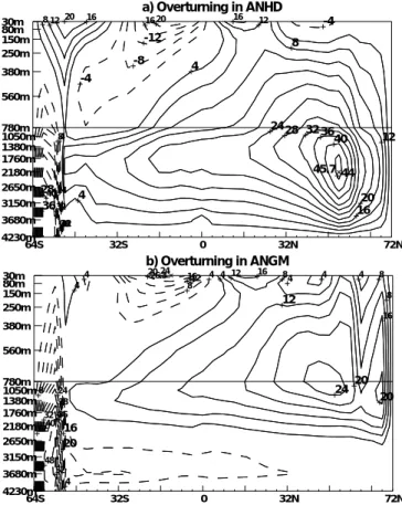
et al., 2000). The meridional overturning
is stronger in ANHD than in ANGM case (46 Sv versus 26 Sv; see Figure 5). Deep-ocean temperature is about 2ßC colder in ANGM, and the vertical temperature contrast is larger. The sharper vertical temperature contrast in ANGM compensates for the weaker circulation, so that heat transports in the two cases are close to each other (Jiang
et al., 1999; Kamenkovich et al., 2000).
Two important differences are also observed in the ACC region in
agreement with the results of
Danabasoglu and McWilliams (1995). First, the deep convection, which is active in this region in ANHD, is eliminated in ANGM. Second, in
ANHD, there are two strong overturning cells in the Southern Ocean. First is a
4 4 8 8 12 12 12 16 16 16 20 20 24 28 32 36 40 44 40 3632 2824 20 20 16 16 12 -12 8 -8 4 -4 -4 45.7 30m 80m 150m 250m 380m 560m 780m 1050m 1380m 1760m 2180m 2650m 3150m 3680m 4230m 64S 32S 0 32N 72N a) Overturning in ANHD 4 4 4 4 4 8 8 8 12 12 16 16 20 20 24 52 48 44 40 36 32 28 24 24 20 20 16 16 12 12 8 8 4 4 26.3 4 30m 80m 150m 250m 380m 560m 780m 1050m 1380m 1760m 2180m 2650m 3150m 3680m 4230m 64S 32S 0 32N 72N b) Overturning in ANGM
Figure 5. Annual mean of the global meridional
overturning streamfunction (Sv). (a) ANHD;
(b) ANGM (eddy-induced transport velocities
are added). Contour interval is 4 Sv; negative contours are shown as dashed lines.
wind-driven Deacon Cell, which has a transport of 18 Sv at its maximum near the surface at 52ßS and extends to 1000 m depth. The Deacon Cell is partially cancelled by eddy-induced transport velocities in ANGM with its transport being less than 6 Sv. There is an additional circulation pattern induced by the presence of the ridge in the Drake Passage and bottom drag applied everywhere in the ACC. The strength of this cell depends mainly on the speed of the ACC, which is around 220 Sv for either experiment, and shows little difference between the two cases.
This reduction in the convection and vertical advection in the Southern Ocean should result in weaker vertical mixing of tracers in ANGM, as suggested by McDougall et al. (1996). As will be seen below, reduced vertical mixing leads to noticeable differences in the model response to climate change.
The main features of the atmospheric circulation produced in both cases are very similar to each other and to those obtained in a present-day climate simulation with the atmospheric model alone (Sokolov and Stone, 1998). This is not surprising, since, as mentioned above, the simulated SST in both cases is very close to its observed values.
In both the ANGM and ANHD simulations, sea ice formation takes place only in the points treated by a mixed layer ocean model while no sea ice is formed in the 3D ocean model domain. As a result, the simulated latitudinal extent of the sea ice is somewhat smaller than both the observed, and that obtained in a present-day climate simulation with the atmospheric model coupled to a mixed layer ocean model.
3.2 Direct Coupling: Causes for the Climate Drift. Experiments DIRGHD and DIRGM Similar to the anomaly-coupled experiments, we conduct directly coupled experiments with two mixing schemes: HD scheme (experiment DIRHD) and GM scheme (experiment DIRGM). Due to differences in the surface fluxes produced by the atmospheric component and those used for the spin-up of the oceanic component, the coupled model with either mixing scheme
undergoes a considerable adjustment during the entire 200 years of the initial spin-up. 3.2.1 Surface Response
The globally-averaged SST reaches a quasi-equilibrium state after the first 150 years of integration (Figure 4), with the variations smaller than 0.2ßC. The values of SST are, however, noticeably different from the observed ones.
The initial mismatch between oceanic heat transport and that implied by the atmosphere prior to coupling is the main reason for the systematic deviation of temperature from its observed values. The heat flux into the ocean in the atmosphere-only run is plotted in Figure 6, together with the divergence of the heat transport per meter of longitude (in W/m2), in two ocean-only experiments. Note that the difference between SST simulated in the coupled run and the observed values is the largest (reaching 5.5ßC; Fig. 6b) to the north of 40ßN, where the mismatch between heat fluxes also has a maximum. Due to the large thermal inertia of the ocean, its heat transport does not change and remains convergent north of 40ßN during the initial stage of coupling. This convergence is
-80 -60 -40 -20 0 20 40 60 80 -100 -80 -60 -40 -20 0 20 40 60 80 Latitude W/m 2 a) Heat Flux -80 -60 -40 -20 0 20 40 60 80 -5 0 5 10 15 20 25 30 Latitude ßC b) Sea Surface Temperature from atmosphere in ocean only in ocean onlyHD GM Levitus DIRGM DIRHD
Figure 6. (a) Heat flux (in W/m2) through the lower
boundary of the atmosphere model in its steady, uncoupled state (dashed line with dots); and divergence of the oceanic heat transport (per meter of longitude) in two uncoupled steady states: GM (stars) and HD (squares).
(b) SST (in ˚C) simulated in the directly coupled
present-day climate runs: DIRGM (stars), DIRHD (squares); Levitus SST (solid line with dots).
unbalanced by the surface heat flux; in the atmosphere-only run, the heat flux is positive at 40ßN in Fig. 6a. The result is a warming of the upper ocean layers and the overlying atmosphere. A warmer surface in principle should result in larger heat loss due to outgoing radiation. However, the humidity and cloud cover in the atmosphere (not shown) both increase as a result of the warming. As a result, the long-wave radiative flux from the atmosphere back to the ocean thus intensifies, increasing the greenhouse effect, and maintaining the warm surface temperature anomaly. A similar effect of the mismatch between heat fluxes is observed near the equator, where SST in the coupled run is again larger than the observed.
A similar process leads to the temperature changes at the two southernmost points of the ocean domain (Fig. 6b). The poleward heat transport in this area prior to coupling is larger in the HD case than in the GM case, mainly because of the unrealistic diffusive heat transport in the former case. The heat convergence in the ocean in the coupled state is then unbalanced by a smaller heat loss to the atmosphere (Fig. 6a); the temperature rises as a result. This rise in the water temperature above climate values makes freezing impossible and the sea ice is absent in DIRHD. The extensive convection, which removes water from the cold polar air, further contributes to the absence of the sea ice in the model (Wiebe and Weaver, 1999).
The situation is opposite in the GM case with the heat transport convergence at 62ßS being smaller in amplitude than the cooling at the surface (Fig. 6a). As a result, the SST is colder than its observed values (Fig. 6b) and a significant amount of ice is formed in the DIRGM experiment at the southernmost oceanic grid point at 62ßS. The ice thickness is below 3 m everywhere in the domain with the exception of limited areas with apparently unstable ice growth. The ice thickness in those regions reaches 10 m by the year 200 and then begins to decrease. The zonally averaged ice mass at 62ßS does not reach an equilibrium value with the annual maximum value (reached in October) decreasing from 4500 kg/m2 in year 200 to 2800 kg/m2 in year 275. The annual minimum (reached in March) also decreases from 3000 kg/m2 to 1200 kg/m2. Further integration does not lead to stabilization of the ice mass. The unrealistically small ice cover in the ocean-only run explains the poor representation of sea-ice in this model. We plan to improve this aspect of the model in the future.
It is noteworthy that SST is hardly changed around 30ßN and 30ßS (Fig. 6b), where the mismatch between heat fluxes is also large. The oceanic heat transport in these regions, however, is nearly non-divergent (Fig. 6a) and thus does not lead to any significant temperature changes. This example therefore emphasizes the important role the ocean can have in causing systematic deviations in the temperature field.
3.2.2 Deep Temperature Drift. Experiments DIRGMN and FWFGM
The deep temperatures continue to drift in DIRHD and DIRGM and the total oceanic surface heat flux fluctuates around —1 W/m2
indicating the overall cooling of the ocean. The systematic drift below the surface is the largest in DIRGM, where the deep temperature continues to change throughout the last 75 years of integration with noticeable systematic cooling at the depth of
1500 m and some warming at mid-latitudes in the Northern Hemisphere (Figure 7). In addition, the circulation is also changing with sinking in the North Pacific (NP) slowly increasing (Figure 8b)
together with a systematic increase in NP surface salinity characteristic of many models with climate drift (Manabe and Stouffer, 1988; Stocker et al., 1992). This indicates a possible transition to a circulation pattern different from a conveyor belt with active sinking in both the NA and NP. Although the rate of the temperature drift decreases with time, the drift of the circulation toward a different state dissuaded us from carrying the experiment for longer times.
Figure 7. (at right) Drift in the zonally averaged ocean temperature, computed as a difference between its values averaged over years 266–275 and 201–205. Contour interval is 0.1˚C. Experiment DIRGM.
(a) Pacific; (b) Atlantic.
a) DIRGM: Pacific 0.1 0.1 0.1 0.2 0.3 0.2 0.6 0.5 -0.4 -0.4 -0.3 0.3 -0.3 -0.2 -0.2 -0.1 0.1 -0.4 30m 80m 150m 250m 380m 560m 780m 1050m 1380m 1760m 2180m 2650m 3150m 3680m 4230m 62S 30S 0 34N 70N 0.1 0.1 0.1 0.1 0.2 0.2 0.2 1 0.9 0.9 0.8 0.8 0.7 0.7 -0.6 0.6 0. -0.6 0.5 -0.5 0.4 -0.4 0.3 0.3 0.3 0.2 0.2 -0.1 -0.1--0.7 30m 80m 150m 250m 380m 560m 780m 1050m 1380m 1760m 2180m 2650m 3150m 3680m 4230m 62S 30S 0 34N 70N b) DIRGM: Atlantic
It is noteworthy that the North Atlantic sinking exhibits significantly larger interannual variability in DIRHD case than it does in DIRGM (Fig. 8a). The difference is smaller but still well pronounced in the both present-day climate and climate change anomaly-coupled runs (Fig. 8a and Fig. 18).
As discussed in Section 1, the drift in deep temperature is common for many coupled models. There are a number of reasons for its existence in the directly
Figure 8. (at right) Evolution in time of the maximum (subsurface) meridional overturning during the present-day climate run for experiments: ANGM, ANHD, DIRGM, DIRHD, WFWGM. (a) North Atlantic (first 50 years of DIRHD not shown);
(b) North Pacific.
a) Maximum overturning in North Atlantic
0 50 100 150 200 250 300 10 20 30 40 50 60 70 years Sv ANGM ANHD DIRGM DIRHD WFWGM b) Maximum overturning in North Pacific 0 50 100 150 200 250 300 0 1 2 3 4 5 6 7 8 9 years Sv ANGM DIRGM DIRHD WFWGM ANHD
coupled experiments in our study. The drift is in large part caused by the fact that it takes a long time for the bulk of the ocean to fully adjust to the change in SST that resulted from the mismatch in heat transports of the two component models. In addition, changes in the circulation and formation of ice in DIRGM can each be a significant factor in causing systematic
temperature changes.
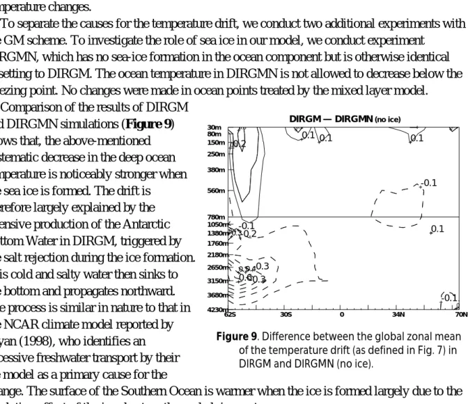
To separate the causes for the temperature drift, we conduct two additional experiments with the GM scheme. To investigate the role of sea ice in our model, we conduct experiment
DIRGMN, which has no sea-ice formation in the ocean component but is otherwise identical in setting to DIRGM. The ocean temperature in DIRGMN is not allowed to decrease below the freezing point. No changes were made in ocean points treated by the mixed layer model.
Comparison of the results of DIRGM and DIRGMN simulations (Figure 9) shows that, the above-mentioned systematic decrease in the deep ocean temperature is noticeably stronger when the sea ice is formed. The drift is
therefore largely explained by the intensive production of the Antarctic Bottom Water in DIRGM, triggered by the salt rejection during the ice formation. This cold and salty water then sinks to the bottom and propagates northward. The process is similar in nature to that in the NCAR climate model reported by Bryan (1998), who identifies an excessive freshwater transport by their ice model as a primary cause for the
0.1 0.1 0.1 0.1 0.1 0.2 0.2 0.3 0.6 0.50.4 0.4 -0.3 0.3 0 -0.2 -0.1 -0.1 0.1 -0.1 -0.3 30m 80m 150m 250m 380m 560m 780m 1050m 1380m 1760m 2180m 2650m 3150m 3680m 4230m 62S 30S 0 34N 70N
DIRGM — DIRGMN (no ice)
Figure 9. Difference between the global zonal mean
of the temperature drift (as defined in Fig. 7) in DIRGM and DIRGMN (no ice).
change. The surface of the Southern Ocean is warmer when the ice is formed largely due to the insulating effect of the ice sheet on the underlying waters.
In the second additional experiment, WFWGM, the moisture flux and wind stress is coupled directly, whereas the heat flux and SST are coupled through anomalies. No sea ice is formed in the ocean model. The drift in the circulation is now present in both basins; in addition to the intensifying sinking in the NP, also present in DIRGM, the sinking in the NA now weakens substantially. The sinking rate in the NA is only 12 Sv at the end of the experiment; the number is close to the NP sinking rate of 8.5 Sv (Fig. 8), which indicates that the circulation is in a state different from a conveyor belt. In contrast, the NA sinking is robust in DIRGM (Fig. 8a).
The adjustments in the heat flux therefore act to slow the NA sinking destabilizing the conveyor belt circulation in the model. A plausible mechanism works as follows. Heat flux adjustments tend to lower SST in the NA with respect to the NP, since heat fluxes in the ocean-only climate are out of NA and into NP (see Fig. 2). The cooling of NA in turn induces the zonal moisture
flux from the Pacific into Atlantic (see Eq. 3 and Figure 10) weakening the sinking. Decrease in the overturning strength leads to the drop in meridional heat and salt transports and further cooling and freshening of the NA. The effect of the freshening of the surface waters in NA wins over that of the cooling and the sinking weakens.
On the other hand, the increase in the NP sinking in the two cases with directly coupled moisture fluxes (DIRGM and WFWGM), indicates that the circulation pattern in ANGM is maintained by the adjustments in the moisture fluxes (Fig. 10). The GFDL coupled GCM exhibits a similar behavior (Manabe and Stouffer, 1988). Large moisture flux into
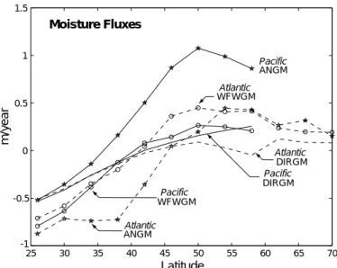
25 30 35 40 45 50 55 60 65 70 -1 -0.5 0 0.5 1 1.5 Latitude Pacific Pacific Pacific ANGM ANGM DIRGM WFWGM WFWGM Atlantic Atlantic Atlantic m/y ear Moisture Fluxes DIRGM
Figure 10. Zonally averaged, annual mean moisture
fluxes into the ocean (m/yr) for: Pacific (solid
lines) and Atlantic (dashed lines); DIRGM, ANGM
(stars), and WFWGM (circles). Mid- to high latitudes of the Northern Hemisphere only.
the NP prevents relatively cold surface waters there from sinking. In contrast, smaller amplitudes of the directly coupled moisture flux through the surface of NP in DIRGM and WFWGM
(Fig. 10) leads to the intensification of sinking in the region. Increased circulation results in the increase in the associated northward salt transport, which acts to further increase salinity and thus enhance the sinking. The systematic positive deviations of the surface salinity in the NP in our directly coupled model are also similar to those reported by Manabe and Stouffer (1988).
The intensifying NP sinking acts to increase the temperature of the deeper ocean layers by bringing down the warm surface waters. The resulting systematic warming of the upper kilometer of the ocean in the mid- latitudes in the Northern Pacific basin is almost identical between DIRGM and WFWGM (see Fig. 7a and Figure 11a). The only difference in warming between DIRGM and WFWGM is explained by the superimposed overall cooling of the ocean in DIRGM. This negative drift in temperature is markedly reduced in WFWGM proving that it is mainly caused by the mismatching heat transports in the uncoupled states of atmospheric and oceanic model components. The remaining cooling of the Atlantic in WFWGM (Fig. 11b) is caused by the weakening NA sinking, which warms the deep ocean.
4. GLOBAL CHANGE EXPERIMENTS
To evaluate the dependence of the models response to external forcing on the sub-grid scale mixing parameterization we performed several simulations with both GM and HD schemes. In all of these simulations, the atmospheric CO2 concentration increases at the rate of 1% per year (compounded) for 75 years; it is kept constant after that and the model is integrated for several hundreds years more. Four simulations were carried out in the anomaly-coupling mode: two with
the standard version of the atmospheric model (simulations ANGM and
ANHD) and two simulations (ANGMH and ANHDH) with the sensitivity of the atmospheric model increased through additional cloud feedback (see Section 2.2). The models sensitivity, defined as the equilibrium surface warming which would be caused by the CO2 doubling in a simulation with the atmospheric model coupled to a mixed layer ocean model, was calculated to be about 2.5ßC and 4.5ßC it these two cases respectively. We also carry out two experiments (DIRGMN and DIRHD) in the directly coupled mode to estimate the dependence of the results on the coupling method. As indicated in the preceding section, in all experiment except DIRGM sea ice is formed only in ocean points treated by
0.1 0.1 0.2 0.3 0.4 0.5 0.6 0.7 -0.3 0.2 -0.2 -0.1 -0.1 -0.1 0.8 30m 80m 150m 250m 380m 560m 780m 1050m 1380m 1760m 2180m 2650m 3150m 3680m 4230m 62S 30S 0 34N 70N a) WFWGM: Pacific 0.1 0 0.1 0.1 0.2 0.3 0.4 -0.3 -0.2 -0.2 0.2 0.1 0 -0.1 -0.1 -0.1 0.1 0.4 30m 80m 150m 250m 380m 560m 780m 1050m 1380m 1760m 2180m 2650m 3150m 3680m 4230m 62S 30S 0 34N 70N b) WFWGM: Atlantic
Figure 11. As in Fig. 7, but for the experiment WFWGM.
a mixed layer ocean model. Therefore, to simplify the analysis of the effects of the mixing scheme in the directly coupled model, we prohibit formation of the sea ice by the 3D ocean model in the directly coupled experiment with the GM scheme (DIRGMN; see also Section 3.2.2). Results of these simulations are discussed in Section 4.1.
Two additional simulations performed with the GM parameterization were devised to study the dependence of our model response on the rate and magnitude of CO2 increase. In one of them (simulation ANGM150) atmospheric CO2 increases at 1% per year for 150 years, in the other (ANGM2) it increases 2% per year for 75 years. In both cases CO2 increases about 4.4 times its
Table 2. Climate Change Simulations
Mixing Fluxes Models CO2 increase Total Length of
Name Scheme Adjusted Sensitivity K Rate Length Simulation
ANGM GM yes 2.5 1% 75 675 ANHD HD yes 2.5 1% 75 675 ANGMH GM yes 4.5 1% 75 675 ANHDH HD yes 4.5 1% 75 675 DIRGMN GM no 2.5 1% 75 75 DIRHD HD no 2.5 1% 75 75 ANGM150 GM yes 2.5 1% 150 675 ANGM2 GM yes 2.5 2% 75 675
initial value. Results of these experiments are compared with the standard experiment ANGM in Section 4.2. Brief descriptions of all climate change
simulations are given in Table 2.
4.1 Response to CO2 Increase Dependence on Parameterization of Sub-grid Scale Mixing 4.1.1 Temperature Response
At the time of CO2 doubling, the increase in the globally averaged surface air temperature (SAT) is slightly larger in the simulations with the GM
parameterization, namely 1.58ßC and 2.2ßC (decadal means for years 66—75) in ANGM and ANGMH versus 1.44ßC and 1.99ßC in ANHDH and ANHD, respectively (Figure 12). Differences in surface warming become more visible during the following integration with the fixed CO2 concentration, especially between simulations with higher climate sensitivity.
The latitudinal distribution of surface warming is, however, noticeably different between the GM and HD cases at the
0 100 200 300 400 500 600 700 -1 0 1 2 3 4 5 6 ANGM ANHD ANGM150 ANGM2 ANGMH ANHDH years ßC
Sea Surface Temperature
Figure 12. Increase in the global mean surface air
temperature for the global change experiments and six stabilization runs: ANGM, ANHD,
ANGM150, ANGM2, ANGMH, and ANHDH. The differences with the correspondent initial values are plotted in each case.
time of CO2 doubling (Figure 13). There is very little inter-hemispheric asymmetry in ANGM and ANGMH simulations, except for somewhat larger warming of Northern Hemisphere due to a larger land area. Land-sea contrast in the surface warming is caused mainly by a large difference in heat capacity between the land and ocean. In contrast, the large difference between warming of the Northern and Southern Hemispheres in ANHD and ANHDH is apparent. Such strong inter-hemispheric asymmetry of the surface response is in fact
characteristic for many models that use HD (e.g., Manabe et al., 1991). Weaker and delayed warming of the high latitudes in the Southern Hemisphere is typical for models with HD and is
-60 -40 -20 0 20 40 60 0.5 1 1.5 2 2.5 3 3.5 4 4.5 5 5.5 Latitude ßC
Transient Warming of Surface Air Temperature
ANHDH ANGM150 ANGM2 ANGM ANGMH ANHD
Figure 13. Transient increase in the zonally averaged
surface air temperature. The decadal means of the difference with the corresponding reference runs (see text) are shown for years 66–75 for all experiments except ANGM150, where the averaging is done for the years 136–145.
explained by the very deep mixed layer in the region created by strong convection and vertical advection (Manabe et al., 1991; McDougall et al., 1996).
The deep heat penetration in the Southern Oceans in ANHD is in fact evident in the vertical structure of the ocean temperature increase (Figure 14a). The upper 1000 m in the Southern Ocean are warmed by more than 0.6ßC. The heating of the deeper layers is even larger; the water below 1000 m is warmed by almost a degree in the two southernmost points most likely by the strong deep convection in the region. Another region of deep heat penetration is the NA, where active
0.1 0.1 0.2 0.3 0.4 0.4 0.5 0.5 0.5 0.6 0.6 0.6 0.7 0. 0.8 0.8 0.8 0.90 0.9 1 1 1 1 1.1 1.1 1.2 1.2 3 0.1 1.4 30 80 150 250 380 560 780 1050 1380 1760 2180 2650 3150 3680 4230 62S 30S 0 34N 70N a) ANHD 0 0.1 0.1 0.2 0.3 0.4 0.5 0 0.6 0 0.70.8 0.9 0.9 1 1 1 1 1.1 1.1 1.1 1 1.2 1.2 1.2 1.41.2 0 0.3 0.2 0.1 1.6 30 80 150 250 380 560 780 1050 1380 1760 2180 2650 3150 3680 4230 62S 30S 0 34N 70N b) ANGM 0.1 0.1 0.1 0.2 0.3 0.3 0.3 0.3 0.4 0.4 0.5 0.5 0.6 0.7 0.8 0.9 1 1.1 1.1 1.2 1.2 1.2 1.3 1.3 1.31.4 30 80 150 250 380 560 780 1050 1380 1760 2180 2650 3150 3680 4230 62S 30S 0 34N 70N c) DIRHD 0.1 0.1 0.2 0.2 0.3 0.30.4 0.4 0.5 0.5 0.5 0.6 0. 0.7 0 0.8 0 0 0.9 0.9 1 1 1.1 1.1 1.2 1.21.3 0.4 0.30.20.1 1.4 30 80 150 250 380 560 780 1050 1380 1760 2180 2650 3150 3680 4230 62S 30S 0 34N 70N d) DIRGMN
Figure 14. Transient increase in the zonally averaged ocean
temperature. The decadal mean for the years 66–75 is shown as a function of latitude and depth for: (a) ANHD; (b) ANGM;
(c) DIRHD; (d) DIRGMN (no ice). Contour interval is 0.1˚C.
sinking of surface waters and deep convection occur. Apart from these two zones, the depth of water volume heated by more than 0.2ßC is between 560 and 780 m. As discussed in Section 3.1, the GM scheme eliminates excessive convection and its eddy-induced velocities cancel the advective effects of the Deacon Cell. These differences in the dynamics of the Southern Ocean result in much weaker vertical mixing of anomalous heat in the ANGM case. As a result, the zone of deep heat penetration in the Southern Ocean is now absent (Fig. 14b). The depth of the water mass heated by more than 0.2ßC is less than 1380 m everywhere to the south of 50ßN. It is noteworthy that the warming is now deeper in the mid- and low latitudes than in ANHD.
Moderate sinking rates in ANGM also result in the warming being shallower in the Northern Atlantic, where it now does not reach all the way to the bottom as it does in ANHD. Differences between deep ocean temperature change in experiments ANHDH and ANGMH (not shown) are qualitatively similar to those described above.
Another interesting feature in ANGM is the presence of the local minimum in the zonally averaged ocean warming at 52ßN (Fig. 14b; somewhat smoothed in Fig. 13). There is a region of local cooling in the western Atlantic at that latitude, where the maximum temperature decrease is about 1.8ßC, which explains the minimum. This regional cooling is concentrated close to the western boundary and is apparently caused by the decrease in the meridional heat transport by the modeled Gulf Stream. Cooling in this region was also observed in other studies with various AOGCMs (Manabe et al., 1991; Cubash et al., 1992; Russell and Rind 1999). Surface warming
in ANHD also has a minimum at the same latitude; there are however no areas of cooling and the minimum in Fig. 14a is much less pronounced. A possible cause for the difference is the strong diapycnal mixing in the HD scheme that erodes horizontal temperature anomalies. In contrast, horizontal mixing in ANGM is minimal in the regions of steep isopycnal surfaces.
The differences in the transient temperature response between DIRGMN and DIRHD directly coupled experiments are qualitatively similar to, but smaller in amplitude than those in the anomaly coupled runs. The vertical circulation in the Southern Ocean in DIRHD case is relatively slow and its difference with DIRGMN is less dramatic than in the anomaly-coupled experiments. The slower circulation is explained by weaker winds over the Southern Ocean, leading to the reduction of both the Deacon Cell and the topographically induced cell in the ACC (see Section 3.1). Weaker circulation results in weaker deep heat mixing in the region, as the transient temperature response shows (compare Figs. 14c and 14a). The penetration of
anomalous warming is however still much deeper in the transient response in the DIRHD than that in the DIRGMN (see Figs. 14c and 14d).
The SAT in ANHD and ANGM simulations continues to increase for more than 500 years after the CO2 concentration is fixed. These changes in SAT are very well correlated with changes in sea ice cover (Fig. 12 and Figure 15). For example, the decrease of SAT in both ANHD and ANHDH simulations during years 80—100 is accompanied by an increase in sea ice cover. Although no sea ice is formed by the 3D ocean model, there are five latitudinal bands in which SST and sea ice are calculated by a zonally averaged mixed layer ocean model. Sea ice cover reaches a stable state after about 500
0 100 200 300 400 500 600 700 1.5 2 2.5 3 3.5 4 4.5 5 5.5 Years Sea ice co v er (%) ANGM ANGMH ANHD ANHDH
Globally Averaged Sea Ice Cover
Figure 15. Globally averaged sea ice cover (in %) as
a function of time: ANGM, ANHD, ANGMH, and ANHDH.
years in ANGM and ANHD runs, while SAT starts to equilibrate some 100 years later. The inter-hemispheric contrast in heating evolves with time but remains different between simulations with GM and HD schemes. In ANGM, both hemispheres warm almost identically for about 400 years when abrupt melting of the sea ice in the Southern Hemisphere (SH) causes an 0.4ßC increase in SH SAT during just about 20 years. In contrast, there is a significant delay in SH warming at the initial stage of ANHD as discussed above. However, after some 150 years SH SAT starts to increase in ANHD at a higher rate than does NH SAT and the local minimum in surface warming at 60ßS disappears. At the same time, the impact of the abrupt ice melting (Fig. 15) on SAT is much smaller here than in ANGM apparently due to the strong deep heat penetration at the southernmost points of the ocean model. The increase in the global mean SAT
averaged for years 666—675 from its values in the corresponding control runs is 2.4ßC and 2.6ßC in ANHD and ANGM respectively. This difference between two simulations is almost entirely due to different warming of the Southern Hemisphere. SAT averaged over the Northern
Hemisphere increases by 2.35ßC and 2.38ßC in ANHD and ANGM simulations, while the corresponding numbers for the Southern Hemisphere are 2.46ßC and 2.82ßC.
The increase in surface temperature for years 666—675 (Figure 16) in ANGM shows the usual equilibrium response high latitude amplification associated with the sea ice/albedo feedback. In ANHD, in contrast, the surface warming decreases nearly monotonically from 60ßN to 60ßS (Fig. 13). As a result, the increase in SAT at 60ßS is 0.8ßC larger in ANGM, while the corresponding difference in SST is more than 1ßC. It is noteworthy that changes in sea ice cover are almost identical in ANGM and ANHD and the difference in the latitudinal structure of the surface warming is therefore a result of different rates of heat uptake by the ocean. Results of the simulations with large climate sensitivities (ANGMH and AMHDH) are qualitatively similar to those discussed
60 40 20 0 20 40 60 80 2 3 4 5 6 7 Latitude ßC
Warming of surface air: years 666–675
ANHDH ANGM ANGM2 ANGM ANGMH ANHD
Figure 16. The decadal means of the difference in
zonal mean surface air temperature with the corresponding reference runs (see text) are shown for years 666–675 (warming stops at year 150 for ANGM150 and at 75 elsewhere).
above. Due to the strong drift in the circulation toward a different climate state (see the next section) in the directly coupled experiments, we do not present here the analysis of the corresponding equilibrium states.
As reported above, in the HD simulations heat penetrates deeper in the ocean at high latitudes of both hemispheres than it does for the GM runs. As a result, the warming at high latitudes in the GM cases is larger in the upper ocean and weaker in the deep layers compared to the HD simulations throughout all simulations. In addition, the deep-ocean warming gradually becomes larger in the HD simulations except for the upper 1500 meters between 30ßS and 50ßS. These changes in the ocean warming are reflected in the temporal structure of the sea level rise due to thermal expansion (Figure 17). While CO2 concentration is rising, sea level rise shows almost no dependence on mixing parameterizations. After CO2 is fixed, the sea level rise becomes somewhat larger in the simulations with the GM scheme; the opposite is true later in the simulations.
Wiebe and Weaver (1999) found larger differences in the deep-ocean warming between their simulations with the HD and GM sub-grid scale mixing parameterizations than we do here. The increase in the volume-averaged global ocean temperature after 500 years is about 50% larger in
their simulations with the HD. The analysis of the changes in the thermohaline circulation helps to understand the difference between the results of Wiebe and Weaver (1999) and those presented here. Knutti and Stocker (1999) show that stronger thermohaline circulation leads to a larger sea level rise. The strength of NA overturning in the present-day climate simulations with HD is about twice as large as in those with the GM parameterization both in our study and in the study by Wiebe and Weaver (1999). However, while in the latter study this ratio hardly changes throughout the global change
0 100 200 300 400 500 600 700 0 0.1 0.2 0.3 0.4 0.5 0.6 0.7 0.8 0.9 1 ANGM ANHD ANGM150 ANGM2 ANGMH ANHDH Sea Le v e l Rise (m) Years
Sea Level Rise
Figure 17. Sea level rise (in meters) due to thermal
expansion for experiments ANGM, ANHD, ANGMH, ANHDH, ANGM2, and ANGM150.
experiments, it decreases down to 1.4 in our model (see next section). The smaller difference in the circulation is then consistent with the smaller contrast in the sea level rise. It should also be noted that our simulations are too short for an accurate estimate of the equilibrium sea level rise.
4.1.2 Changes in the Circulation The thermohaline circulation significantly slows in response to the increase in the atmospheric CO2 concentration, but does not cease completely. The behavior of the sinking in time is noticeably different between experiments with GM and HD schemes. The NA sinking in ANGM (Figure 18) decreases by 5 Sv (20%) by the end of the period with increasing CO2 concentration, while the corresponding change in ANHD is significantly larger and amounts to more than 15 Sv (33%). Changes in the NA overturning are somewhat larger in the experiments with higher climate sensitivity (ANGMH and ANHDH); the difference with the standard cases is however small (about 1 Sv). 0 100 200 300 400 500 600 700 10 15 20 25 30 35 40 45 50 ANGM ANHD ANGM2 ANGM150 ANGMH ANHDH
Maximum North Atlantic Sinking
years
Sv
Figure 18. Evolution in time of the maximum
(subsurface) overturning in the North Atlantic for the global change experiments and following stabilization runs: ANGM, ANHD, ANGM150, ANGM2.
Warming of the atmosphere generally leads to increase in the heat and moisture transports in the NA. Both processes act to decrease surface density in the region, slowing the sinking. As discussed by Dixon et al. (1999), the relative importance of the two processes is different between simulations with various atmosphere-ocean models. To estimate their relative
importance in our model, we conduct additional experiments with the ocean-only model forced by surface fluxes diagnosed from coupled runs. We carry out the experiments in two settings for each mixing scheme. In one setting, the heat and momentum fluxes are taken from the
corresponding reference runs with constant CO2, while the moisture flux is taken from the global change experiments. For both GM and HD schemes, the NA sinking in that case remains nearly constant, closely following that in the reference run. In the second setting, moisture and
momentum fluxes are taken from the reference runs, while the heat flux is taken from the corresponding global change experiments. The decrease of the NA sinking in that case matches that in the global change runs, proving that it is the anomalous heating of the oceanic surface that is the main reason for the slowdown of the thermohaline circulation in our model. It should also be noted that change in runoff is not taken into account in our simulations.
Wiebe and Weaver (1999) suggest that the warming of the surface acts to intensify the NA circulation by increasing the density and pressure contrast between the high latitudes and tropics. This effect, however, depends on the latitudinal distribution of the surface warming. With
uniform warming, the sea level rise would indeed be larger in the tropics due to the nonlinearity of the equation of state. The anomalous surface warming however increases northward (Fig. 13), which acts to decrease the meridional pressure gradient in the upper pycnocline counteracting the effect reported by Wiebe and Weaver (1999). The decrease in the meridional surface density gradient north of 48ßN in the transient state of ANGM and ANHD is consistent with the weakening of the circulation (Figure 19).
The NA sinking starts to recover after the CO2 concentration stabilizes. In ANGM, this recovery begins only about 10 years after the end of the CO2
increase (Fig. 18). The quick start of the recovery is very similar to that in Wood
et al. (1999) in their model with no flux
adjustments, which also uses the GM scheme. By the year 475, the NA sinking in ANGM recovers to 23 Sv, which is 92% of its initial value. In contrast, the recovery is noticeably delayed in ANHD. After 75 years of integration with constant CO2 level during which the NA sinking remains nearly unchanged, the circulation begins
70 60 50 40 30 20 10 0 10 -0.2 -0.15 -0.1 -0.05 0 0.05 0.1 0.15 F w (m/y ear) latitude ANHD ANGM year 76 year 76 ANHD ANGM year 676 year 676
Fresh Water Fluxes
Figure 19. Fresh water fluxes over the Atlantic in the
Southern Hemisphere for experiments ANGM (stars) and ANHD (circles): year 76 (solid) and year 676 (dashed). Units are meters/year.
slowly to recover (see Fig. 18). It is also noteworthy that the NA sinking reaches only 32 Sv, which is 72% of its initial value, over the remaining part of the stabilization run, another noticeable difference with the ANGM case.
A number of physical factors can explain the fast recovery of the circulation in experiment ANGM and the differences in the time-dependence of the circulation with experiment ANHD. Wang et al. (1999) demonstrated that an increase in the surface buoyancy flux into the Southern Hemisphere leads to intensification of the thermohaline circulation in the entire Atlantic.
Significant surface warming (Fig. 16) and an increase of the freshwater flux into the ocean in mid- and high latitudes of the Southern Hemisphere during the stabilization stage of the experiment ANGM (Fig. 19) are then both consistent with the strong recovery of the circulation (Fig. 18). In contrast, a cooler surface and the decrease in the high-latitude downward moisture flux in ANHD (Fig. 19) act to reduce the circulation according to Wang et al. (1999). Strong warming of the Southern Hemisphere in experiment ANGM (Fig. 16) also enhances the meridional pressure gradient at low latitudes (Wiebe and Weaver, 1999), which drives more flow in the meridional direction. Another plausible mechanism contributing to a weak recovery in experiment ANHD is related to the excessive horizontal cross-isopycnal diffusion in the high latitudes of NA. The existence of deep convection in the region is crucial for the operation of the thermohaline circulation. The diffusion however tends to remove heat anomalies from the deep part of the water column enhancing its stability and therefore acting to reduce convection; the diapycnal mixing is in contrast small in the GM scheme.
As in the anomaly-coupled runs, the NA sinking weakens initially in the directly coupled experiments. However, we do not observe a following recovery as we do in the anomaly-coupled experiments. In addition, the strengthening of the NP overturning cell continues and reaches levels close to those in NA by the end of year 475. The circulation therefore, switches to the state with active sinking in the northern parts of both model basins. Due to this drastic change in the circulation patterns, a detailed comparison with the anomaly-coupled cases does not seem reasonable in the present study.
4.2 Dependence of Model Response on the Rate of the CO2 Increase
The temperature response shows the usual dependence on the rate of CO2 increase
(Schmittner and Stocker, 1999; Stouffer and Manabe, 1999), namely for a given total increase in CO2 the warming is slightly larger for a lower rate (Fig. 16). In our simulations, the surface temperature rises by 1.4ßC and 1.6ßC at the time of CO2 doubling and by 3.6ßC and 4.1ßC at the time of CO2 quadrupling for 2% and 1% per year rates correspondingly. Warming of the deep ocean shows an even stronger dependence. At the same time, NA sinking (Fig. 18) slows down from about 25.5 Sv at the beginning of the experiments to about 21 Sv by the time of CO2
doubling and to 15.5 Sv at the time of CO2 quadrupling regardless of the rate. In simulations with the GFDL AOGCM (Stouffer and Manabe, 1999) reduction in the strength of the thermohaline circulation (THC) caused by doubling of CO2 increases with decrease in the rate of CO2 change.
As a whole, changes in the NA sinking in simulations with the standard version of our model are smaller than those produced by the GFDL AOGCM (Manabe and Stouffer, 1994 and
Stouffer and Manabe, 1999); but are similar to those obtained in the simulations with the
HadCM3 AOGCM (Wood et al., 1999). For example, in simulations with both the HadCM3 and our model (ANGM2 and ANGM150) quadrupling of CO2 leads to a rather moderate decrease in the strength of THC followed by its recovery; in the simulation with the GFDL AOGCM, in contrast, THC collapses completely. Since the HadCM3, as well as the standard version of our model uses GM scheme, while the GFDL model employs HD, the differences in the behavior of THC are likely explained by the use of the different sub-grid mixing parameterizations. It was shown in the previous section that the response of the circulation to the increase in the external forcing is much larger when HD is used. In particular, changes in the strength of THC (relative to its initial value) during the first 70 years of experiments ANHD and ANHDH are very similar to those in analogous simulations with the GFDL AOGCM. A similar, but weaker, dependence of the changes in circulation on the sub-grid mixing scheme was obtained in simulations carried out by Wiebe and Weaver (1999). Our results also agree well with those of the simulation with ECHAM3/LSG AOGCM (Mikolajewicz and Voss, 1998) in which NA sinking decreases by about 12 Sv by the 15 years after the CO2 is quadrupled.
The fact that in the ANGM2 simulation NA sinking continues to slow down for a longer time after CO2 is fixed but recovers faster than in the ANGM150 simulation is in agreement with results of Stouffer and Manabe (1999). An interesting feature of the ANGM150 simulation is that the thermohaline circulation starts to recover after 130 years of integration despite the continuing increase in CO2 concentration. In an analogous simulation by Wiebe and Weaver (1999), the circulation starts to recover after 90 years of integration, that is some fifty years before CO2 concentration quadruples.
5. SUMMARY AND CONCLUSIONS
We have introduced a coupled atmosphere/ocean model of intermediate complexity, which is sufficiently efficient computationally to allow a large number of multiple-century integrations; but, in contrast with most models of intermediate complexity, is capable of reproducing most physical processes simulated by coupled atmosphere-ocean GCMs. The use of flux-adjustment technique prevents the model from a systematic drift and keeps the surface temperature close to the observed values. The thermohaline circulation in the present-day climate simulations remains steady with the maximum magnitude of the overturning 27 Sv and 44 Sv in the GM and HD cases respectively. Asynchronous integration of oceanic momentum and tracer equations is feasible as long as the ratio between the time steps for the tracer and momentum remains not very large (12 in our case).
Given the crude spatial resolution and simplifications made in both components of the model described here, it is not surprising that our directly coupled model shows systematic deviations in the temperature field both on and below the surface. Such a drift is characteristic even for the most sophisticated contemporary coupled AOGCMs. Initial disagreement between the heat flux