Impact of different convective cloud schemes on the simulation of the tropical seasonal cycle in a coupled ocean-atmosphere model.

HAL Id: hal-00184738

https://hal.archives-ouvertes.fr/hal-00184738

HAL is a multi-disciplinary open access archive for the deposit and dissemination of sci-entific research documents, whether they are pub-lished or not. The documents may come from teaching and research institutions in France or abroad, or from public or private research centers.

L’archive ouverte pluridisciplinaire HAL, est destinée au dépôt et à la diffusion de documents scientifiques de niveau recherche, publiés ou non, émanant des établissements d’enseignement et de recherche français ou étrangers, des laboratoires publics ou privés.

Pascale Braconnot, Frédéric Hourdin, Sandrine Bony, Jean-Louis Dufresne,

Jean-Yves Grandpeix, Olivier Marti

To cite this version:

Pascale Braconnot, Frédéric Hourdin, Sandrine Bony, Jean-Louis Dufresne, Jean-Yves Grandpeix, et al.. Impact of different convective cloud schemes on the simulation of the tropical seasonal cycle in a coupled ocean-atmosphere model.. Climate Dynamics, Springer Verlag, 2007, 29, pp.501-520. �10.1007/s00382-007-0244-y�. �hal-00184738�

Impact of different convective cloud schemes on the

simulation of the tropical seasonal cycle with a coupled

ocean-atmosphere model

P. Braconnot1*, F. Hourdin2, S. Bony2, J.-L. Dufresne2, J.-Y. Grandpeix2, and O. Marti1

1. IPSL/LSCE, unité mixte CEA-CNRS-UVSQ, Bât.712, Orme des Merisiers, 91191

Gif-sur-Yvette Cedex. * Corresponding author.

2. IPSL/LMD, case 99, 4 place Jussieu, 75252 Paris cedex 01.

Abstract.

The simulation of the mean seasonal cycle of sea surface temperature (SST) remains a challenge for coupled ocean-atmosphere general circulation models (OAGCMs). Here we investigate how the numerical representation of clouds and convection affects the simulation of the seasonal variations of SST. For this purpose, we analyze the simulations of two versions of the same OAGCM differing only by their convective cloud schemes. Most of the differences between the two simulations in the mean atmospheric temperature and precipitation fields reflect differences found in atmosphere-only simulations. They affect the ocean interior down to 1000 m.

Substantial differences are found between the two coupled simulations in the seasonal march of the Intertropical Convergence Zone in the eastern part of the Pacific and Atlantic basins, where the equatorial upwelling develops. The results show that the convergence of humidity between ocean and land during the American and African boreal summer monsoons plays a key role in maintaining a cross equatorial flow and a strong windstress along the equator. An other important factor is the presence of low level clouds in subsidence regions over cold waters south of the equator, which favors the maintenance of a cross equatorial SST gradient and of a surface wind convergence north of the equator. The results suggest that the inhibition of convection by downdraughts, as well as radiative feedbacks between clouds and SST, have a key role on the relative distribution of large-scale convection between ocean and land, and thereby the dynamics of the equatorial upwelling and the SST seasonal cycle in the Pacific and Atlantic oceans.

1. Introduction

The representation of clouds and atmospheric convection has been emphasized as a critical issue for the simulation of the current climate in various coupled ocean atmosphere models (IPCC 2001). In particular coupled models have a tendency to produce a warm bias in the eastern Pacific and Atlantic oceans where the equatorial upwelling develops from the eastern border (Latif et al. 2001; Davey et al. 2002). The representation of the seasonal cycle of Sea surface temperature (SST), such as the representation of the seasonal evolution of the equatorial upwelling in the eastern Pacific remains a challenge for coupled simulations. It is an example of a coupled ocean-atmosphere variability potentially strongly affected by the numerical representation of clouds and convection. Indeed, the existence of the cold tongue along the equator is an annual response of the climate system to the semi-annual forcing of incoming solar radiation at the top of the atmosphere in this region. It results from complex atmosphere-ocean interaction (Wang 1994). Two modes have been identified so far that shape the seasonal evolution of SST in this region (Wang 1994; Nigam and Chao 1996). The first one is related to the monsoon circulation that converges in central America. This mode represents the tropical part of a global response of the atmosphere-land-ocean system to the differential insolation between the northern and southern hemisphere (Wang 1994). The second mode results from large-scale air-sea interactions, and involves the relationship between SST gradients and wind, the latent heat flux and the presence of a stratocumulus deck in the subsiding regions of the east Pacific. Several studies have shown that the interactions between low-level moisture , stratocumulus deck and cloud radiative properties contribute to the maintenance of the cold tongue (Ma et al. 1996; Yu and Mechoso 1999; Gordon et al. 2000).

In that vein, we investigate how atmospheric convection and clouds impact the large-scale atmospheric and oceanic circulation in the tropical regions, using two versions of a coupled ocean-atmosphere models differing only by the parameterisation of convective clouds. The corresponding simulations show substantial differences in the tropical circulation. In particular the seasonal evolution of the Intertropical Convergence Zone (ITCZ) in the eastern part of the tropical Pacific

and Atlantic is more confined towards the equator in one of the simulations and the strength of the equatorial upwelling is damped. The comparison of these two simulations allows us to check how this is related to the land-sea contrast and to the simulation of cloud cover in the eastern Pacific. The objective of the paper is thus to highlight differences in the adjustment of the ocean-atmosphere system to convective cloud schemes, and to show how the interaction between clouds, convection and the large-scale circulation affects the characteristics of the mean climate and of the mean seasonal cycle in tropics.

We use the last version of the IPSL coupled ocean-atmosphere model (Marti et al. 2005). Its atmospheric component, LMDZ, has been recently improved as described by Hourdin et al. (2006). The Tiedke (1989)’s convection scheme, originally implemented in the LMDz atmospheric model by Li (1999), was carefully tuned so that it was possible to run a millennium time scale coupled simulation with a previous version of the IPSL coupled model, for which sea-ice was prescribed to climatological values and the land surface was represented using a simple bucket model (Li and Conil 2003). Replacement of the Tiedke (1989)’s scheme by the Emanuel (1993)’s scheme greatly improved the large scale distribution of tropical precipitation in simulations with the atmospheric model. In particular, the Inter Tropical Convergence zone (ITCZ) is less confined along the equator with the Emanuel ‘s scheme, and precipitations are better reproduced over the Amazonian basin (Hourdin et al. 2006). The rate of warming and moistening of the atmospheric column by convection shows substantial differences between the two schemes, particularly over ocean. This difference is particularly marked over ocean, where the convective downdraughts of the Emanuel's scheme decrease the surface layer moist static energy much more that those of the Tiedtke's scheme. Analyses of atmosphere-alone simulations with the two convection schemes suggest that these differences are at the origin of substantial differences in the simulation of the land-sea contrast in convection and of the large scale tropical atmospheric circulation (Hourdin et al. 2006). Our purpose here is to analyse how these differences impact the simulated climate when the atmosphere is coupled to the ocean.

The remainder of the manuscript is organized as follows. Section 2 presents a short description of the coupled model, with emphasis on the convection and cloud schemes, and on the major characteristics of the simulations. Differences in the tropical circulation simulated with the two convection schemes are analysed in section 3. Section 4 discusses differences in the timing and in the amplitude of the tropical seasonal cycle. The mechanisms responsible for the differences in the seasonal march of the Intertropical Convergence Zone (ITCZ) in the eastern equatorial Pacific and Atlantic oceans are discussed in section 5. Comparison with atmosphere alone simulations helps us to understand the role of the interactions between convection and the large scale circulation in the tropics. The conclusion is provided in section 6.

2. Model and simulations

Model description

Simulations were performed with the last version of the coupled model developed at Institut Pierre Simon Laplace (IPSL, Paris Marti et al. 2005). IPSL_CM4 couples the grid point atmospheric general circulation model LMDz (Hourdin et al. 2006) developed at Laboratoire de Météorologie Dynamique (LMD, France) and the oceanic general circulation model ORCA (Madec

et al. 1998) developed at Laboratoire d'Océanographie Dynamique et de Climatologie (LOCEAN,

France). On the continent, the land surface scheme ORCHIDEE (Krinner et al. 2005) is coupled to the atmospheric model. Only the thermodynamic component of ORCHIDEE is active in the simulations presented here. The evolution of the carbon cycle and the dynamics of the vegetation are not considered. The closure of the water budget with the ocean is achieved thanks to a river routing scheme implemented in the land surface model. A sea-ice model (Fichefet and Maqueda 1997), which computes ice thermodynamics and dynamics, is included in the ocean model. The ocean and atmospheric models exchange surface temperature, sea-ice cover, momentum, heat and fresh water fluxes once a day, using the OASIS coupler (Terray et al. 1995) developed at CERFACS (France). None of these fluxes is corrected.

Compared to previous versions of the IPSL model (Braconnot et al. 2000; Dufresne et al. 2002), the coupling scheme was revisited to ensure both global and local conservations of momentum, heat and fresh water fluxes at the air-sea interface. Following some of the ideas implemented in previous model versions (Dufresne and Grandpeix 1996; Braconnot 1998), an interface model was implemented in the atmospheric model. Each atmospheric grid box accounts for up to four different subsurface types: ocean, land, sea-ice, and land ice. Surfaces fluxes are computed according to the surface characteristics (roughness length, stability etc..). The interpolation scheme conserves the heat and water budget both globally and locally (Marti et al. 2005).

In its present configuration, the model is run at medium resolution. The atmospheric grid is regular, with a resolution of 3.75° in longitude, 2.5° in latitude, and 19 vertical levels. The ocean model grid has approximately 2 degrees resolution (0.5 degrees near the equator) with 184 points in longitude, 142 points in latitude and 31 1evels in the ocean.

Convection and cloud scheme

The coupled model is run either with Emanuel’s or Tiedke’s convection scheme. These schemes both belong to the category of "mass flux schemes". They parameterize the convective mass fluxes as well as the induced motions in the environmental air. In the Tiedtke's (1989) scheme, only one convective cloud is considered, comprising one single saturated updraught. Entrainment and detrainment between the cloud and the environment can take place at any level between the free convection level and the free sinking level. There is also one single downdraught extending from the free sinking level to the cloud base. The mass flux at the top of the downdraught is a constant fraction (here 0.3) of the convective mass flux at cloud base. This downdraught is assumed to be saturated and is kept at saturation by evaporating precipitation. The version of the Tiedtke's scheme used here is close to its original formulation and uses a closure in moisture convergence. Triggering is a function of the buoyancy of lifted parcels at the first grid level above condensation level.

In the Emanuel’s scheme, the backbone of the convective systems is regions of adiabatic ascent originating from some low-level layer and ending at their level of neutral buoyancy. Shedding from these adiabatic ascents yields, at each level, a set of draughts which are mixtures of adiabatic ascent air (from which some precipitation is removed) and environmental air. These mixed draughts move adiabatically up or down to levels where, after further removal of precipitation and evaporation of cloud water, they are at rest at their new levels of neutral buoyancy. In addition to those buoyancy-sorted saturated draughts, unsaturated downdraughts are parameterized as a single entraining plume of constant fractional area (here 1% of the grid cell) driven by the evaporation of precipitation. The version of the Emanuel's scheme used here is very similar to Emanuel (1993). Closure and triggering take into account both tropospheric instability and convective inhibition. Our version differs from the original one in the removal of most explicit grid dependencies (e.g. the lifting condensation level varies continuously and not from grid level to grid level), which yields a smoother variation of convection intensity with time and a weaker dependence on vertical resolution.

The cloud scheme of the model is a statistical cloud scheme that describes the subgrid-scale distribution of total water by a generalized log-normal distribution, whose variance and skewness are diagnosed, and that uses zero as the lower bound of the distribution. Non-convective clouds are predicted by imposing that the statistical moments of the total water distribution are a function of the vertical profile of total water and of saturated specific humidity (Hourdin et al. 2006). The non-convective clouds are exactly the same whatever the convection scheme used. Clouds associated with cumulus convection are predicted differently depending on the convection scheme used in the GCM. When using the Emanuel’s scheme, the cloud scheme is coupled to the convection scheme by diagnosing the variance and the skewness of the total water distribution from the vertical profile of in-cloud water content predicted by the convection scheme and from the degree of saturation of the large-scale environment (Bony and Emanuel 2001). In the case of the Tiedke’s scheme, an homogeneous cloud fraction is assumed between cloud base and cloud top, that is a function of the

vertically-integrated moistening tendency predicted by the Tiedtke's convection scheme (Hourdin et

al. 2006).

Cloud microphysical properties are computed as described by Bony and Emanuel (2001, Table 2 for water clouds and case "ICE-OPT" of Table 3 for ice clouds): temperature thresholds (-15°C and 0°C) are used to partition the cloud condensate into liquid and frozen cloud water mixing ratios; cloud optical thickness is computed by using an effective radius of cloud particles set to a constant value for liquid water clouds (12 μm in the simulations presented here), and decreasing with decreasing temperature (from 60 to 3.5 μm) for ice clouds. The vertical overlap of cloud layers is assumed to be maximum-random. A more complete description of these schemes can be found in Hourdin et al. (2006).

Simulations

We consider two coupled simulations run with these two schemes. Both schemes are equivalent from a global energetic point of view. This means that the coupled model is equilibrated and that long term integrations are possible without using any flux correction at the air-sea interface.

The simulation with the Emanuel’s scheme, referred to as KE, corresponds to the reference version of the IPSL model that has been used for the production of IPCC AR4 scenarios (Dufresne

et al. 2005; Swingedouw et al. 2006). This simulation will then be considered as the reference. It is

a 500 year long simulation. Over this period, the model drift in global mean surface temperature is less than 0.02 °C/century. The simulation is stable with a global mean 2m air temperature of 14°C that presents low frequency variability of about 0.1 to 0.2°C around this mean. In the following, we will consider a mean seasonal cycle computed from the last 200 years of the simulation.

The simulation with the Tiedke scheme (TI) was run for 300 years. The initial state and the spin up strategy is the same as for KE. The model drift is negligible, but larger than for the KE simulation (0.05°C/century). The global mean temperature is warmer (15.7 °C) and the low frequency variability smaller. We will consider the last 150 years of the simulation in the remainder

of this manuscript. When needed, the results will be compared with the atmosphere-alone simulations presented by Hourdin et al. (2006).

Simulated climate: global characteristics.

Figure 1 shows the difference between the simulated annual mean sea surface temperature (SST) and the Levitus (1982)’s climatology for the two simulations. The large-scale patterns of the SST field are successfully captured by the two model versions in most places.

The major default of the reference simulation (KE) is the cold bias in the mid latitudes both in the Atlantic and Pacific oceans (Figure 1a). Locally, this bias reaches 6 °C in the North Atlantic, which results from the conjunction of a southward shift of the north Atlantic drift and the advection of cold water from the Gin and the Labrador seas. It has been attributed to a lack of deep water formation in the Labrador Sea (Swingedouw et al. 2005), caused by an overestimation of the atmospheric fresh water budget over the North Atlantic, the Nordic seas and the southern part of Greenland. This excessive fresh water input creates a thin halocline at the surface, which reduces the local buoyancy of surface waters, and thus ocean convection. Note that the equatorward shift of the mid-latitude stormtracks is already present in atmosphere alone simulations. It is amplified when the atmospheric model is coupled to the ocean and leads to the mid latitude cold SSTs in both hemisphere. The shift reduces when increasing horizontal resolution (not shown).

This cold bias is not as large in the TI simulation (Figure 1b). On the contrary, surface waters are too warm along the margin of sea-ice in the southern hemisphere and in the northern part of the Pacific ocean. The root mean square differences (rms) between the simulated map and Reynold’s (1988) observations suggest that TI better reproduces global SST with a global rms of 1.4 °C against 1.7 °C for KE. When the rms is computed over the tropical regions (30°S-30°N), the rms is 1.5 °C for TI and 1.2 °C for KE. This suggests that model biases are primarily located in mid-latitudes in KE, whereas they occur at most mid-latitudes in TI.

The major differences between the two coupled simulations and observations follow the differences highlighted in atmosphere-alone simulations (Hourdin et al. 2006). For example, figure

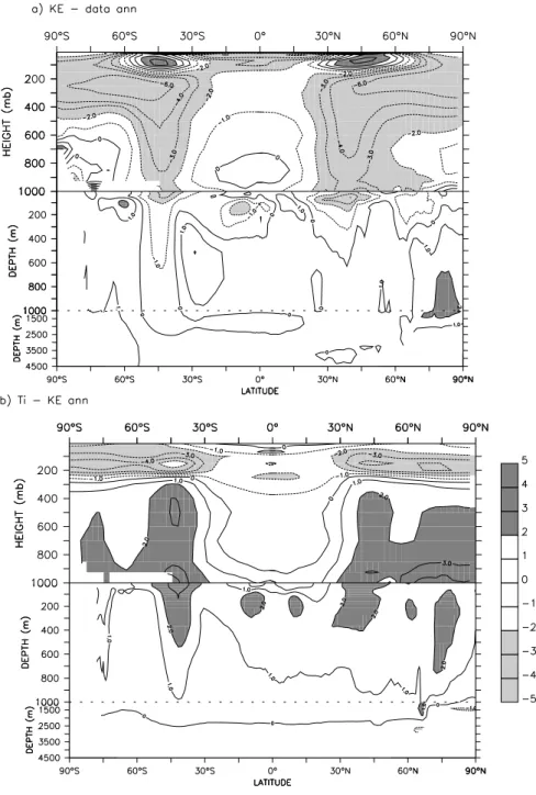
2a shows that in KE the zonal mean temperature presents a cold bias of up to 8°C at about 200hPa. This pattern was attributed to too large moisture content at these levels and is amplified by the coupling with the ocean. Differences in the atmosphere have their counterpart in the ocean. The KE simulation presents a slight cold bias on the first 400 m of the ocean around 30°N and 40°S, consistent with the cold atmospheric bias (Figure 2a). Elsewhere in the ocean, the departure from climatology doesn’t exceed 2°C, except at high latitudes, where the warm bias at depth reflects the lack of deep water formation.

Figure 2b also reveals that in middle and high latitudes, the TI simulation is associated with even colder conditions in the upper troposphere and lower stratosphere and warmer conditions in the lower and middle troposphere than the KE simulation. The TI simulation is also characterized by warmer water in the first 1000 m of the ocean with maximum value in the two regions of intermediate water formation noted above. It is less satisfactory at depth were 1°C warmer than observed water is found down to 1000 m.

The equator-to-pole differences in the tri-dimensional structure of temperature in the ocean and atmosphere is associated with large-scale differences in the dynamics of the two fluids. In particular, the northward heat transport is larger in KE, both in the atmosphere and in the ocean. These differences reach about 1PW at 20°N. For this aspect, KE is in better agreement with Trenberth and Solomon (1994) estimate of the heat transport from satellite observation and reanalysis.

3. Large scale features in the tropics

Large scale features of the simulated climate compared to observations.

The model performs well in the tropics. In KE, errors are less than 0.5°C over most of the basins (figure 1a). The exception is at the eastern side of the equatorial Pacific and Atlantic were the warming indicates that the equatorial upwelling is not well located along the coast. This is a classical bias of coupled model, especially with the relatively coarse resolution we are using here (Latif et al. 2001). The equatorial section of annual mean temperature plotted as a function of depth

(figure 3) shows that the vertical temperature gradient is more diffuse than in the observation. However, the shape of the thermocline presents an east-west gradient in agreement with observation both in the Pacific and Atlantic oceans. In the latter, warm surface waters accumulate in the first ocean layers in the eastern part of the Gulf of Guinea and the upwelling is shifted to the west. The surface ocean temperature as well as the east-west temperature gradient at depth are also satisfactorily reproduced in KE in the Indian ocean (Figure 3b).

Figures 1 and 3c show that TI is slightly warmer than KE in the eastern Pacific and colder over the warm pool. As a result, the East-West SST gradient is reduced by about 1.4 °C in TI compared to KE across the Pacific. There is even more difference between the two simulations in the ocean interior (Figure 3). For example, the 14°C isotherm depth is located about 100m deeper in the eastern part of the Pacific Ocean, suggesting that the upwelling is not strong enough. In the Atlantic TI produces a flat thermocline across the basin. This bias leads to a reversal of the temperature gradient at the surface compared to observation, and the equatorial upwelling nearly vanishes. Also the temperature gradients are reversed across the Indian ocean in the first 200 m, with warmer water in the eastern part. This rapid comparison shows that the thermocline depth is on average deeper in TI than in KE, which suggests that the local thermal inertia of the ocean is slightly higher in this simulation.

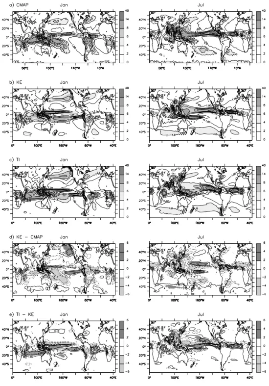
The large scale characteristics of wind stress and precipitation (Figure 4 and 5) are consistent with the temperature field. KE reproduces the broad features found in observations. In January, the trade winds are well reproduced in the Pacific ocean except in the eastern part where they penetrate too far south (Figure 4b, left). This structure is consistent with the lack of precipitation north of the equator in this region and with the presence of a double ITCZ structure around 4°S (Figure 5b and d, left). Along the coast of South America and South Africa the northward component of the windstress is not strong enough (Figure 4b, left). The coastal upwelling is thus slightly damped and the surface SST warmer than observed (Figure 1a). The windstress structure also is too zonal between 4°S and the equator in the western Pacific in January (Figure 4b, left), consistent with the zonal distribution of the southern Pacific convergence zone (SPCZ, Figure 5c and d, left). In July,

the observed windstress is more intense in the southern hemisphere and up to 8°N in the eastern Pacific and Atlantic Ocean (Figure 4a, right). This pattern is associated with the strengthening of the northern hemisphere Hadley cell, and with the intensification of the monsoon flow from the ocean towards the continent, where heavy precipitation occurs (Figure 5a, right). This return flow from the ocean to the continents over America and Africa is reproduced in KE. However, windstress is not strong enough along the eastern border in July (Figure 4b, right), consistent with the accumulation of warm water in these regions and with the westward shift of the core of the upwelling (Figure 1a). Figure 5d also shows that monsoon rainfall is underestimated over the southern border of North America, Africa and India.

These drawbacks are more pronounced in TI. In January the trade winds are too strong in the northern hemisphere and converge too far south (Figure 4c, left), which is consistent with the southward shift of the ITCZ between the two simulations (Figure 5e, left) and with the too strong precipitation over the maritime continent (Fig. 5c left). The maximum wind stress is also slightly shifted from the middle of the basin to the west, and there is almost no extension of the eastward (or the westerly) winds in the western Pacific (Fig. 4c, left). The zero line for both the zonal and meridional components of the wind stress (not shown) is shifted to the south by about 5°degrees of latitude. The Walker cell across the Indian Ocean is weaker in this simulation, which explains the reversal of the temperature gradient in the ocean interior (Figure 3). The same weakening was obtained in atmosphere-alone simulations. In July the return flow from the ocean to the continent associated with the American and African monsoon is not strong enough (Fig. 4c, right). In the Atlantic the Southeaststerlies do not penetrate far enough during summer in the northern hemisphere. The wind stress is thus not strong enough along the equator and does not allow for the development of the equatorial upwelling at the coast. It is also interesting to note that the ITCZ is shifted to the south in TI compared to KE year round compared to KE in the Pacific ocean (Figure 5e). It is consistent with the too intense trade winds, their excessive extension in the southern hemisphere in January, and their lack of northern extension in the eastern Pacific in July.

The above discussion shows that representation of convective clouds in the model affects the simulation of the tropical climate, and that the monsoon flow over the ocean, the July monsoon precipitation over Central America and Africa, and the development of the equatorial upwelling in the eastern Pacific and Atlantic oceans are connected. We analyze below how this connection affects the seasonal cycle of SST in the eastern Pacific and Atlantic.

Mean seasonal cycle.

Figure 6 shows the mean seasonal evolution of SST and precipitation for several regions in the tropics. The phasing of the annual cycle of SST and precipitation is satisfactorily represented for KE in most regions. However, as discussed above (comments of figure 1 and 5), precipitation is underestimated in the West Pacific north of the equator from April to October. In the eastern part of the basin, they are overestimated from January to June. This excessive precipitation is associated with an excessive surface warming during the same period. This feature corresponds to the double ITCZ structure that develops over a longer period and with a larger magnitude than in the observations. A similar feature is present in the Atlantic ocean, where the SST is too warm from November to June and where the precipitation is overestimated from January to June south of the equator. The phasing of the annual mean cycle of SST and precipitation is less satisfactory in TI. In particular the development of the double ITCZ and the associated warm surface conditions lasts longer in this simulation and the magnitude is larger. The differences found in the Indian ocean in SST (figure 1b and 3), are also associated with a misrepresentation of the double peak of SST in this basin.

We display the geographic distribution of the seasonal cycle of the simulated SST in the tropics and compare it with observations in figure 7. For simplicity, we characterize the seasonal cycle and assess it against observations by considering its magnitude (quantified here as the difference between the monthly maximum and the monthly minimum temperature estimated from a mean seasonal cycle) and the correlation between the simulated and observed seasonal cycles of SST. Results for the magnitude are plotted for each grid point as the ratio of the difference from

observation over the observation. Figure 7a, b and c show that the two model versions tend to underestimate the magnitude of the seasonal cycle in the eastern part of the Pacific and Atlantic oceans, where SSTs are warmer than observed (Figure 1). This underestimate reaches up to 50% in TI over large regions, whereas, it is around 20% in KE. On the other hand, the magnitude tends to be overestimated in the western part of the basin. In the western Atlantic, we note an excessive magnitude of the seasonal cycle in KE which is due to the westward shift of the equatorial upwelling. The correlation between the observed and simulated seasonal cycles of the SST characterizes the ability of the model to reproduce the phasing of the seasonal SST anomalies. Figures 7 d and e show that it is better in KE in most places.

The evolution of the seasonal cycle along the equator averaged between 2°N and 2°S (Figure 8) shows that both simulations produce a timing of the equatorial upwelling in phase with the observations. However the westward shift of the upwelling core in the Pacific is more pronounced in TI, as is the westward propagation with time (Figure 8). From experiments with an intermediate coupled model, Fu and Wang (2001) suggested that the westward propagation of the cold tongue was mainly due to the zonal advection of cold water by the oceanic circulation. This is the case in TI where the zonal current is more intense west of 140°W due to the stronger trade winds in these regions (Figure 4). In the Atlantic, the magnitude and the phase of the equatorial upwelling are satisfactory in KE although its core is shifted to the west. As already noted, this equatorial upwelling nearly vanishes in TI.

4. Tropical Oceans and seasonal march of the ITCZ

Seasonal march of the ITCZ in the eastern Pacific.

The analysis of the mean seasonal cycle shows that the convection and cloud schemes strongly impact the representation of both the mean state and the seasonal characteristics of the climate in the eastern part of the Pacific ocean. We now analyse this in more depth, considering first the region extending from 110 °W to 90 °W and 8°S to 14 °S in the eastern Pacific (shaded in figure 6). This region allows us to analyze the development of the equatorial upwelling and the connection

between the equatorial SST and the location of the ITCZ. In this region SST has a well defined seasonal cycle, with warmer water located south of the equator in boreal spring and extending to the north of the equator from June to September when the equatorial and coastal upwelling intensifies from 8°S to 2°N in boreal summer and autumn (Figure 9).

Several aspects of the wind and cloud fields have been identified as important players in this feature. The upwelling along the coast of Peru and the equatorial upwelling in the east fully develop when the wind is along the coast of South America and its strength intensifies to the north. At that time, the zonal component of the windstress also intensifies along the equator towards the west, which enhances the equatorial divergence and allows for the strengthening of the equatorial upwelling further west. The onset of American summer monsoon on the continent at 15°N seems to be an important factor in this intensification and in the position of the core of the equatorial upwelling near the coast (Wang 1994). Several feedbacks, involving SST, clouds or wind and evaporation enter then into play to reinforce the upwelling and maintain the ITCZ in a northern position (e.g. Xie and Saito 2001).

We first consider KE. As already seen in figure 8, the seasonal evolution of the equatorial upwelling is quite realistic in this simulation. In particular, the northward SST gradient between the cold tongue and the warmer water to the north is present in KE from July to November (Figure 9). This is consistent with the onset and the maintenance of the cross equatorial monsoon flow in this simulation (Figure 4). Note however that the structure is slightly shifted towards the equator, and that warm waters do not extend far enough to the north of 8°N, as suspected from the wind stress and the lack of precipitation over the continent (Figure 5). During the time when the SST gradient intensifies to the north (April-May), precipitation follows quite closely the region of maximum surface warming in the northern hemisphere. In boreal winter and early spring, the maximum precipitation is located as in the observations above warm waters around 4°S, peaking in March.

Figure 10 also shows that in KE the total cloud cover intensifies within the ITCZ and also south of the equator over the cold waters from July to October. In the latter regions, air is subsiding and clouds are limited to lower tropospheric levels. They reduce the incoming solar radiation at the

ocean surface and locally favour the surface cooling. Therefore this version of the model produces an annual variation of low level clouds consistent with a local strengthening of the meridional circulation in the eastern Pacific as shown by Ma et al. (1996).

The two model versions exhibit a different behaviour in this region. Interestingly, the first part of the northward shift of the warm waters from their equatorial position to 8°N in April-May is also well reproduced in TI (Figure 9c, left), but as soon as the ITCZ intensifies to the north, the whole structure shifts back to a more equatorward position and the SST gradient becomes flat. Then the ITCZ develops over a kind of SST plateau with no well-defined SST gradient. The reduced SST gradient locally reduces the wind stress along the equator and the equatorial divergence, which contributes to damp the development of the equatorial upwelling. Also large differences are found between the two simulations in the representation of the cloud cover (Figure 10). In TI the maximum cloud cover follows the ITCZ (it is thus maximum where deep convection occurs). Figure 10 also shows that during the peak development of the equatorial upwelling these differences in cloud cover between the two simulations lead to a 80W/m2 difference in net surface shortwave flux across the equator. Therefore in TI the seasonal evolution of the cloud cover damps the SST gradient across the equator, and thereby reduces the strength of the wind along the equator and the strength of the equatorial upwelling.

Figure 11 summarizes the differences along 95°W during the peak development of the upwelling (August-November). Even though KE exhibits systematic differences with observations, it exhibits sharp SST and 2 m air temperature gradient across 2°N. Precipitation over the ocean properly follows the observations. Low level specific humidity increases northwards, with maximum values around 8°N and minimum values in the southern hemisphere. Several characteristics found in KE are in good agreement with the data reported by Pyatt et al (2005) along 95°W. Specific humidity is however slightly overestimated (by about 2g/kg) compared to observation. On the other hand neither the flat SST distribution across the equator nor the uniform distribution of humidity found in TI are realistic. In this simulation, the convergence of humidity,

the maximum precipitation, and surface cooling by radiative fluxes occur at the same location (about 4°N).

Seasonal march of the ITCZ in the Atlantic.

The equatorial Atlantic shares some similarities with the eastern Pacific both at the annual and interannual time scales (Chiang and Vimont 2004). Since in KE the equatorial upwelling develops in the middle of the basin rather than along the coast (Figure 8), we adjusted a box so as to capture its seasonal evolution. Figure 9 and 10 consider thus the zonal average of surface conditions between 30°W and 7°E. The northern limit is provided by the position of the continent in the northern part of the Golf of Guinea (5°N), so that we limit the latitudinal extension from 12°S to 2°N. Therefore the intensity of the equatorial upwelling is slightly reduced in the observation since the core of the upwelling is located further east. However, the seasonal evolution of SST and precipitation is well depicted on these figures. From January to June, warm waters and precipitation associated with deep convection within the ITCZ expand down to 8°S. From July to November, cold waters develop from 8°S to 1°N and warm waters and precipitation are located further north (Figure 9).

For this basin, differences in the representation of the equatorial upwelling and in the location of the ITCZ between TI and KE are quite similar to those found in the eastern Pacific (Figures 9 and 10). They are even larger. In KE, the seasonal march of the ITCZ over this region follows quite closely that of the SST. The timing of the north-south migration of the ITCZ across the equator is well represented. It corresponds to the intensification of the trade winds across the equator and to the eastward convergence of the wind onto the African continent (Figure 4, right) where monsoon precipitation occurs (Figure 5). The monsoon flow and the precipitation do not develop as far north as in the observation, which explains why the zero line of the SST field in figure 9 (right) does not cross 2°N. During the peak of the upwelling, when warm waters and the ITCZ are in their northern position, cloud cover intensifies both in the ITCZ and over the cold waters just south of the equator.

In the latter regions these clouds reduce the incoming solar radiation at the surface and contribute to cool the surface. In TI, the upwelling does not develop and convection is maximum over a flat SST gradient, like in the Pacific ocean. The overall feature is consistent with the windstress field (Figure 4). In TI, the windstress is not strong enough across and along the equator, and so is the return flow towards Africa. The convection is more active over the ocean in TI than in KE, as shown by the 500 hPa large-scale vertical velocity in figure 10. The differences in cloud cover also reveal that the cloud cover develops within the ITCZ in TI. The net effect of these clouds is to damp the meridional SST gradient in this simulation (Figure 10).

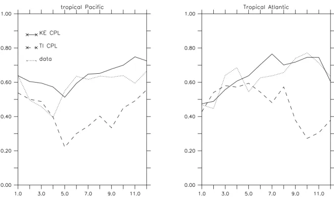
Convection and precipitation in KE are strongly linked to SST. To investigate the link between SST and rainfall, we compute for each month the correlation between SST and rainfall over the tropical (30°S-30°N) Atlantic and Pacific for the two simulations (Figure 12). We also compute this correlation from CMAP (Xie and Arkin 1996) climatology of precipitation and Reynolds’ (1988) climatology of SST. Figure 12 shows that the seasonal evolution is quite satisfactorily represented in KE. The slight overestimate suggests that this parameterisation is too sensitive to the local moist static energy which is mainly controlled by the SST (Biasutti et al. 2006). This common model bias is associated with a tendency for a too strong coupling between rainfall and low level humidity and a too small coupling with the free troposphere humidity. On the other hand, the correlation is poor for TI, and even not significant during boreal summer, certainly because SST has no well defined structure in the equatorial regions in this simulation. During boreal winter the convergence occurs where SST is maximum south of the equator near South America, which explains the better correlation found for this period.

5. Interaction between convection, clouds and the large scale circulation

The analyses of the seasonal evolution of the equatorial upwelling in the eastern Pacific and equatorial Atlantic show that KE and TI exhibit similar differences in the two basins. The seasonal cycle of the equatorial upwelling is better reproduced in the simulation where the cross equatorial wind stress is stronger, and in which the wind convergence toward the continent is sustained. This is

in agreement with Xie and Saito (2001), who show that the presence of a bulge of landmass was important to determine the meridional structure of the ocean ITCZ in the east, and with Fu and Wang (2001), who identified the meridional wind stress as a critical parameter in the development of the equatorial upwelling in the east Pacific.

The differences between the two simulations presented here involve the connection between cross-equatorial trade wind, the monsoonal returned flow over southern North America or West Africa, and the cloud cover. The way the convection and cloud schemes interact with the large-scale circulation is to produce such differences is further discussed from atmosphere-alone results (Hourdin et al. 2006). Then we discuss the ocean feedback.

Link with the characteristics of convection and cloud radiative forcing.

We first compare the behaviour of tropical clouds and convection simulated in the atmospheric and coupled versions of the model. To segregate regimes of deep convection and upper-level cloud tops from regimes of shallow convection and low-level clouds, we use the compositing methodology of Bony et al. (2004), which considers the monthly mean 500 hPa vertical velocity (ω500) as a proxy for large scale vertical motions in the atmosphere. For the different circulation regimes, we compare the mean cloud radiative forcing (CRF) and probability distribution function (PDF) of ω500 derived from coupled and uncoupled experiments with each version of the convective cloud schemes (Figure 13).

For the different regimes, both the PDF and the CRF of the coupled simulations are similar to the ones found in the atmosphere alone simulations. In KE the PDF and the CRF are overestimated (up to 12 Wm-2 for the latter) in regimes of moderate convection. In regimes of precipitating convection (ω500 < 20 hPa/day), the net CRF at the top of the atmosphere from TI is more negative (by about 10Wm-2) than that from KE and satellite data. Figure 13c shows that this difference at the top of the atmosphere partly translates to the surface (the SW CRF at the surface is more negative in TI than in KE). This suggests that in TI, the cloud cover of the ITCZ contributes more to cool the surface and to reduce the SST gradient with surrounding areas than in KE. This is consistent with

the colder conditions found in the west Pacific in TI (Figure 1). In subsidence regimes, on the contrary, TI underestimates the cooling effect of clouds, which also contributes to reduce the SST gradient. The way convection affects the warming and moistening of the atmospheric column is also very similar between the coupled and uncoupled simulations, both over the ocean and over land (not shown).

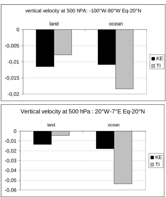
Analyses of the atmosphere-alone simulations by Hourdin et al. (2006) suggest that the better representation of land-sea contrasts in rainfall and cloud radiative forcing with the Emanuel’s scheme comes from the representation of downdraughts over the ocean. In KE convection is inhibited by downdraughts both over land and over the ocean. In TI the inhibition by downdraughts is not present over the ocean and convection is not limited, which explains that stronger ascents may be found in this simulation where convection occurs over ocean (Figure 10). Because of these differences, convection in TI is better sustained over ocean than over land while in KE it is comparable over ocean and land, which contributes to reinforce convection over the more continental northern hemisphere on the average. Figure 14 shows that, as for the atmosphere-alone simulations, convection is more active in TI over ocean, whereas similar ascending motions are found in KE over ocean and land. The situation is event more contrasted for TI in the Atlantic. This effect is more pronounced in the coupled simulations because of the feedback with SST, as explainsed below.

Role of the monsoon flow and low level clouds in the eastern part of the Pacific and

Atlantic

In KE, several feedbacks from the atmospheric circulation come into play in the coupled model to cool down SST along the equator and enhance the SST gradient in KE in the East Pacific and Atlantic. In TI the feedbacks act to damp the SST gradients and the ITCZ remains in a rather south position. These feedbacks involve the ocean circulation and the cloud cover.

Figure 15 shows that in August-September, during the peak development of the upwelling, the zonal currents in the first layer of the ocean model (first 10 m) are smaller in KE than in TI in the

eastern Pacific. The reversal of the westward south equatorial current and the eastward north equatorial current is located at 4°N against 3°N in TI. On the contrary, the meridional component of the current, and the vertical velocity at the base of the first layer are stronger in KE across the equator (Figure 15). Upwelled waters cool the surface, and the meridional component of the current advects northwards cold water from the south of the equator. The meridional windstress component across the equator and its northwards convergence are thus two critical features that help maintain cold water along the equator and a sharp SST gradient to the north of it. This SST gradient locally enhances the windstress. The role of vertical and meridional temperature advection in cooling the surface layer is less active in TI. Also since the thermocline is more diffuse in TI upwelled waters are warmer, reducing the cooling effect of the upwelling. Note that in the Atlantic ocean, the components of the currents are more similar between the two simulations. The major differences come from warmer upwelled waters in the first layer.

As seen in section 4, the cloud cover further contributes to enhance the SST gradient in KE and to damp it in TI. In KE, the SST gradient between the cold equatorial waters and the regions further north is reinforced by the presence of low level clouds over cold waters. The stronger SST gradient maintains the wind stress and the development of the equatorial upwelling. In TI, the development of the equatorial upwelling is not sufficient to maintain a sharp cross equatorial SST gradient that would reinforce the windstress. In addition convective clouds strongly cool down the surface where convection occurs, which further contributes to weaken the SST gradient, and to reinforce the southward shift of the ITCZ.

6. Conclusion

The comparison of two coupled ocean-atmosphere simulations performed with different convective clouds schemes allows us to investigate how the representation of clouds and convection interacts with the large-scale tropical atmospheric and oceanic circulations.

We show that, to first order, the major characteristics of surface climate simulated by the coupled model are primarily controlled by atmospheric processes model. Indeed the distribution of

cloud radiative forcing and convection regimes in the tropical regions is the same between the coupled simulations and simulations with the atmospheric model forced by prescribed SST. In addition several features of the atmospheric simulations are only slightly affected by the coupling with the ocean. This includes in particular the annual mean and the seasonal evolution of the atmospheric temperature, of the precipitation, of the cloud radiative forcing and of the surface wind. The key role of atmospheric processes on coupled simulations has been noted in other studies considering several ocean models and various aspects of the simulated climate. From a set of several state of the art coupled model simulations where models shared either the same atmosphere or the same ocean, Guilyardi et al. (2004) found that the atmosphere has a dominant role in setting El Niño characteristics (periodicity and base amplitude) and errors (regularity). From an analysis of climate sensitivity under global warming with different combinations of the NCAR models, Meehl et al. (2004) concluded the atmospheric model "manages'' the relevant global feedbacks including sea ice albedo, water vapor, and clouds, and that for global sensitivity measures, the ocean, sea ice, and land surface play secondary roles, even though differences in these components can be important for regional climate changes.

In the simulations presented here, differences in the atmospheric simulations propagate down to about 1000m in the ocean interior. The simulated mean state and the seasonal cycle of the SST in most part of the equatorial ocean differ strongly depending on the convection and clouds scheme used. Our results show that the cross equatorial wind in the eastern Pacific and in the Atlantic during boreal summer is critical to maintain the equatorial upwelling, and the advection of cold waters to the north of the equator. The simulation that best represent the position of the ITCZ in these region is the simulation for which this cross equatorial circulation is more active, which maintains a sharp SST gradient in the northern hemisphere. This simulation also exhibits a weaker zonal circulation along the equator. The dominant feature is the link between large scale ocean and continental patterns. In particular, these patterns are connected during summer through the large scale monsoon flow in the eastern equatorial Pacific and Atlantic oceans. Therefore a good

representation of the land sea contrast and of the large scale circulation in the tropics is a key to properly simulate the seasonal cycle over the eastern part of the ocean.

Our analysis also shows that the interaction between convection, clouds and the large scale tropical circulation dominate the differences at the seasonal time scale. In the simulation where convection heating and moistening is inhibited by downdrafts both over the continent and the ocean (KE), the monsoon flow converging in south North America and Africa is better reproduced, and this reinforces the maintenance of the inland moisture convergence. In the simulation (TI) where convection is not inhibited by downdraft over the ocean, convection and moisture convergence are too strong over the ocean, and favor the large scale convergence over the ocean at the expanse of the continent. The ITCZ is thus located further south all year round in this simulation. This mechanism is reinforced by the radiative impact of the cloud cover. In one case (TI) the cloud cover tends to cool the surface in (warm) regions of convection whereas in the other case (KE), low-level clouds in (cold) subsidence regions reinforce the SST gradient between convective regions and their surroundings, which reinforces the windstress and the equatorial upwelling. In both cases the feedback from the ocean circulation leads to SST patterns that enhance these basic mechanisms.

These results clearly show that understanding the coupled system requires to consider in an integrated way the evolution of the seasonal cycle over land and over ocean, since they are interconnected through the atmospheric large-scale circulation. The investigation of the relative strength of deep convection between ocean and land in several models is thus likely to help us to understand why different climate models produce different mean climate states and seasonal cycles in the tropics. Our analysis also suggests that a model assessment should be based on the evaluation both on the assessment of the model's climatology and on the assessment of on both the comparison of simulated climate fields with observations, as well as on key mechanisms. The comparison with climatology reveals that both simulations have serious biases compared to observations. However, when going into the details, it becomes clear that the KE simulation better represents several major features of the mean climate and of the seasonal cycle in the tropical regions. The differences in the parameterisation between these two simulations also have an impact on the interannual variability

simulated by the coupled model. This will deserve future investigation, and will be considered in a forthcoming study.

Acknowledgement. We would like to thank all IPSL people who participate to the development of

the IPSL_CM4 model. We also thank Laurent Fairhead for the introduction of the convection schemes in the LMDZ model, and Ionela Musat for the adjustments of the climatology. Computer time was provided by Centre National de la Recherche Scientifique (IDRIS computing center) and Commissariat à l’Energie Atomique (centre CCRT computing center).

References

Barkstrom, B. R. (1984). The earth radiation budget experiment (erbe). Bull. Am. Meteorol. Soc 65: 1170-1185.

Biasutti, M., A. Sobel and Y. Kushnir (2006). Agcm precipitation biases in the tropical atlantic. Journal of Climate 19(No. 6): 935-958.

Bony, S., J. Dufresne, H. Le Treut, J. Morcrette and C. Senior (2004). On dynamic and thermodynamic components of cloud changes. CLIMATE DYNAMICS 22(2-3): 71-86.

Bony, S. and K. A. Emanuel (2001). A parameterization of the cloudiness associated with cumulus convection; evaluation using toga coare data. Journal of the Atmospheric Sciences 58(21): 3158-3183.

Braconnot, P. (1998). Tests de sensibilité avec le modèle d'atmosphère du lmd, en vue d'améliorer le couplage avec l'océan. note technique IPSL 2: 39.

Braconnot, P., J. Joussaume, O. Marti and N. de Noblet (2000). Impact of ocean and vegetation feedback on 6 ka monsoon changes. Canada, WCRP-111, WMO/TD-No. 1007.

Chiang, J. and D. Vimont (2004). Analogous pacific and atlantic meridional modes of tropical atmosphere-ocean variability. JOURNAL OF CLIMATE 17(21): 4143-4158.

Davey, M. K., M. Huddleston, K. R. Sperber, P. Braconnot, F. Bryan, D. Chen, R. A. Colman, C. Cooper, U. Cubasch, P. Delecluse, D. DeWitt, L. Fairhead, G. Flato, C. Gordon, T. Hogan, M. Ji, M. Kimoto, A. Kitoh, T. R. Knutson, M. Latif, H. Le Treut, T. Li, S. Manabe, C. R. Mechoso, G. A. Meehl, S. B. Power, E. Roeckner, L. Terray, A. Vintzileos, R. Voss, B. Wang, W. M. Washington, I. Yoshikawa, J. Y. Yu, S. Yukimoto and S. E. Zebiak (2002). Stoic: A study of coupled model climatology and variability in tropical ocean regions. Climate Dynamics 18(5): 403-420.

Dufresne, J.-L. and J.-Y. Grandpeix (1996). Raccordement des modèles thermodynamiques de glace, d'océan et d'atmosphère. Note Interne 205, L.M.D.

Dufresne, J., J. Quaas, O. Boucher, S. Denvil and L. Fairhead (2005). Contrasts in the effects on climate of anthropogenic sulfate aerosols between the 20th and the 21st century. GEOPHYSICAL RESEARCH LETTERS 32(21): -.

Dufresne, J. L., P. Friedlingstein, M. Berthelot, L. Bopp, P. Ciais, L. Fairhead, H. Le Treut and P. Monfray (2002). On the magnitude of positive feedback between future climate change and the carbon cycle. Geophysical Research Letters 29(10): art. no.-1405.

Emanuel, K. A. (1993). A scheme for representing cumulus convection in large-scale models. Journal of Atmospheric Science 48(2313-2335).

Fichefet, T. and M. A. M. Maqueda (1997). Sensitivity of a global sea ice model to the treatment of ice thermodynamics and dynamics. Journal of Geophysical Research-Oceans 102(C6): 12609-12646.

Fu, X. and B. Wang (2001). A coupled modeling study of the seasonal cycle of the pacific cold tongue. Part i: Simulation and sensitivity experiments. JOURNAL OF CLIMATE 14(5): 765-779.

Gordon, C., A. Rosati and R. Gudgel (2000). Tropical sensitivity of a coupled model to specified isccp low clouds. JOURNAL OF CLIMATE 13(13): 2239-2260.

Guilyardi, E., S. Gualdi, J. Slingo, A. Navarra, P. Delecluse, J. Cole, G. Madec, M. Roberts, M. Latif and L. Terray (2004). Representing el nino in coupled ocean-atmosphere gcms: The dominant role of the atmospheric component. Journal of Climate 17(24): 4623-4629.

Hourdin, F., I. Musat, S. Bony, P. Braconnot, F. Codron, J. L. Dufresne, L. Fairhead, M. A. Filiberti, P. Friedlingstein, J. Y. Grandpeix, G. Krinner, P. Le Van, Z. X. Li and F. Lott (2006). The lmdz4 general circulation model: Climate performance and sensitivity to parametrized physics with emphasis on tropical convection. Climate Dynamics: in press.

IPCC (2001). Climate change 2001, the scientific basis, Cambridge University press.

Krinner, G., N. Viovy, N. de Noblet-Ducoudre, J. Ogee, J. Polcher, P. Friedlingstein, P. Ciais, S. Sitch and I. Prentice (2005). A dynamic global vegetation model for studies of the coupled atmosphere-biosphere system. GLOBAL BIOGEOCHEMICAL CYCLES 19(1): -.

Latif, M., K. Sperber, J. Arblaster, P. Braconnot, D. Chen, A. Colman, U. Cubasch, C. Cooper, P. Delecluse, D. DeWitt, L. Fairhead, G. Flato, T. Hogan, M. Ji, M. Kimoto, A. Kitoh, T. Knutson, H. Le Treut, T. Li, S. Manabe, O. Marti, C. Mechoso, G. Meehl, S. Power, E. Roeckner, J. Sirven, L. Terray, A. Vintzileos, R. Voss, B. Wang, W. Washington, I. Yoshikawa, J. Yu and S. Zebiak (2001). Ensip: The el nino simulation intercomparison project. Climate Dynamics 18(3-4): 255-276.

Levitus, S. (1982). Climatological atlas of the world ocean, NOAA Professional paper, Washington D.C.

Li, X. (1999). Ensemble atmospheric gcm simulations of climate interannual variability from 1979 to 1994. Journal of Climate 12: 986-1001.

Li, Z. X. and S. Conil (2003). A 1000-year simulation with the ipsl ocean-atmosphere coupled model. Annals of Geophysics 46(1): 39-46.

Ma, C. C., C. R. Mechoso, A. W. Robertson and A. Arakawa (1996). Peruvian stratus clouds and the tropical pacific circulation: A coupled ocean-atmosphere gcm study. Journal of Climate 9(7): 1635-1645.

Madec, G., P. Delecluse, M. Imbart and C. Levy (1998). Opa 8.1 ocean general circulation model reference manual. Note du Pôle de modélisation, Institut Pierre-Simon Laplace 11: 94 pp. Marti, O., P. Braconnot, J. Bellier, R. Benshila, S. Bony, P. Brockmann, P. Cadule, A. Caubel, S.

Denvil, J. L. Dufresne, L. Fairhead, M. A. Filiberti, M.-A. Foujols, T. Fichefet, P. Friedlingstein, H. Goosse, J. Y. Grandpeix, F. Hourdin, G. Krinner, C. Lévy, G. Madec, I. Musat, N. deNoblet, J. Polcher and C. Talandier (2005). The new ipsl climate system model: Ipsl-cm4. Note du Pôle de Modélisation n 26, ISSN 1288-1619.

Meehl, G. A., W. M. Washington, J. M. Arblaster and A. X. Hu (2004). Factors affecting climate sensitivity in global coupled models. Journal of Climate 17(7): 1584-1596.

Nigam, S. and Y. Chao (1996). Evolution dynamics of tropical ocean-atmosphere annual cycle variability. Journal of Climate 9(12): 3187-3205.

Pyatt, H. E., B. A. Albrecht, C. Fairall, J. E. Hare, N. Bond, P. Minnis and J. K. Ayers (2005). Evolution of marine atmospheric boundary layer structure across the cold tongue-itcz complex. Journal of Climate 18(5): 737-753.

Reynolds, R. W. (1988). A real time global sea-surface temperature analysis. Journal of Climate 1: 75-86.

Swingedouw, D., P. Braconnot, P. Delecluse, E. Guilyardi and O. Marti (2005). Sensitivity of the atlantic thermohaline circulation to global freshwater forcing. Climate Dynamics.

Swingedouw, D., P. Braconnot and O. Marti (2006). Sensitivity of the atlantic meridional overturning circulation to the melting from northern glaciers in climate change experiments. Geophys. Res. Lett. 33, No 7.

Terray, L., E. Sevault, E. Guilyardi and O. Thual (1995). The oasis coupler user guide version 2.0. Cerfacs technical report TR/CMGC: 95-46.

Tiedke, M. (1989). A comprehensive mass flux scheme for cumulus parameterization in large-scale models. Monthly Weather Review 117: 1179-1800.

Trenberth, K. and A. Salomon (1994). The global heat balance: Heat transports in the atmosphere and ocean. Climate Dynamics 10: 107-134.

Wang, B. (1994). On the annual cycle in the tropical eastern central pacific. Journal of Climate 7(12): 1926-1942.

Xie, P. and P. Arkin (1996). Analyses of global monthly precipitation using gauge observations, satellite estimates, and numerical model predictions. JOURNAL OF CLIMATE 9(4): 840-858. Xie, S. and K. Saito (2001). Formation and variability of a northerly itcz in a hybrid coupled agcm:

Continental forcing and oceanic-atmospheric feedback. JOURNAL OF CLIMATE 14(6): 1262-1276.

Yu, J. Y. and C. R. Mechoso (1999). Links between annual variations of peruvian stratocumulus clouds and of sst in the eastern equatorial pacific. Journal of Climate 12(11): 3305-3318.

Figure caption.

Figure 1: Annual mean sea surface temperature difference (°C) between a) KE and the Levitus (Levitus 1982) climatology and b) Ti and KE. Values larger (lower) than 2°C (-2°C) are dark (light) shaded. Dashed (solid) lines stand for negative (positive) values.

Figure 2: Annual mean atmosphere and ocean temperature (°C), zonally averaged and plotted as a function of latitude and depth, a) difference between KE and climatology, b) difference between Ti and KE. Note that the first 1000 m of the ocean are expended. Values larger (lower) than 2°C (-2°C) are dark (light) shaded.

Figure 3: Equatorial section of the first 350 meters of the ocean averaged between 2°N and 2°S for a) Levitus’ climatology, b) KE and c) TI. Isolines are plotted every 2°C. Values higher than 14°C are shaded.

Figure 4: January (left) and July (right) wind stress (in Pa) between 30°N and 30°S for a) ERS data, b) KE, and c) Ti.

Figure 5: January (left) and July (right) precipitation (mm/d) for a) the CMAP climatology (Xie and Arkin 1996), b) KE, c) Ti, d) differences between KE and climatology and e) differences between Ti and KE. In all plots isolines are plotted every 2mm/d (the zero line is omitted).

Figure 6: Comparison of annual mean evolution of SST (°C) and precipitation (mmd-1) for KE (solid line), TI (dashed line) and observations (dotted line), for several boxes over the tropical ocean. The box limits are identified as dotted rectangles on the map. The two boxes represented by solid lines correspond to the limits of the regions used to in section 4.

Figure 7: Comparison of the characteristics of the simulated mean seasonal cycle of SST with the Reynold’s (1988). a) Annual mean cycle as estimated from data, b) and c) ratio of the difference between the simulated and observed annual mean SST amplitude (defined as the maximum monthly temperature minus the minimum monthly temperature) to the observed amplitude for TI and KE respectively. d) and e) correlation between the simulated seasonal cycle at each model grid point with the observation for TI and KE. The data have been interpolated on the model grid. Solid lines stand for positive values, dashed lines for negative values and, in c) and b), the heavy solid line represent the 0 correlation.

Figure 8: Seasonal mean evolution (annual mean removed) of SST (°C) along the equator averaged between 2°N-2°S for a) Reynolds ‘ (1988) climatology b) KE and c) TI.

Figure 9: Annual mean evolution of SST (annual mean of the box removed; isolines; °C) and precipitation (shading; mm/d) averaged from a)-c) 90°W to 110°W in the Pacific and e)-f) 30°W to 7°E in the Atlantic and plotted as a function of latitude and time for a) the Reynold’s SST and CMAP precipitation climatologies, b) KE and c) TI.

Figure 10: Same as figure 9 but for a)-c) and e)-g) the seasonal mean evolution of ω500hPa (hPa d -1

, isolines) and total cloud fraction (shading) and d) and h) the difference between the surface net shortwave flux between TI and KE. For shortwave, the annual mean value over the region was subtracted from each simulation to better emphasise the gradients

Figure 11: Cross equatorial section averaged from 90°W to 110°W and from August to November of a) SST (°C) b) 2 m air temperature (t2m,°C) c) precipitation (Precip, mm/day), d) 2m air specific humidity (q2m, g/kg), e) net radiation at the surface (Wm-2, positive downward), and f) the meridional latent heat transport integrated over the atmospheric column (vq, gm-1s-1). In each graph, the solid line represents KE and the dashed line TI. In a) and c) the dotted line stands for the observations (CMAP for precipitation and Reynolds for SST).

Figure 12: spatial correlation between precipitation and SST computed for each month between 30°N and 30°S for a) the Pacific ocean and b) the Atlantic ocean. The solide lines represent the estimation from KE, the dashed line the results from TI and the dotted line an estimate from the Reynold’s (1988) and CMAP climatologies.

Figure 13: Regime sorted plots as a function of ω500 in hPa/d between 30°N and 30°S over the ocean for a) the probability distribution function of ω500, b) the net cloud radiative forcing a the top of the atmosphere (Wm-2), c) the net cloud radiative forcing at the ocean surface (Wm-2). In all graphs the black lines stand for simulations with the Tiedke convection scheme and the red lines for simulations with the Emanuel convection scheme. In figure a) and b) the coupled simulations are represented by the solid lines and AMIP type simulations with the atmospheric model by the dotted lines. For comparison two estimates from ERA40 and NCEP reanalyses for ω500 and ERBE (Barkstrom 1984) for cloud radiative forcing are included.

Figure 14: Bar charts representing the 500 hPa (hPas-1) vertical velocity averaged over land and ocean from June to October in TI and KE for the eastern Pacific and Atlantic. The boxes are respectively 100°W-80°W; 0°N-20°N for the Pacific and 20°W-7°E; 0°N-20°N for the Atlantic.

Figure 15: Ocean currents for the first upper layer of the ocean model and SST in August in the Pacific and Atlantic. a) zonal current in the first model layer (m.s-1), b) meridional current in the first model layer (m.s-1), c) vertical velocity at the base of the first layer (m.d-1), and d) SST (°C). In a), b) c), dark grey represents positive values and light grey negative values.

(Levitus, 1982) climatology and b) Ti and KE. Values larger (lower) than 2°C (-2°C) are dark (light) shaded. Dashed (solid) lines stand for negative (positive) values.

Figure 2: Annual mean atmosphere and ocean temperature (°C), zonally averaged and plotted as a function of latitude and depth, a) difference between KE and climatology, b) difference between Ti and KE. Note that the first 1000 m of the ocean are expended. Values larger (lower) than 2°C (-2°C) are dark (light) shaded.

Figure 3: Equatorial section of the first 350 meters of the ocean averaged between 2°N and 2°S for a) Levitus’ climatology, b) KE and c) TI. Isolines are plotted every 2°C. Values higher than 14°C are shaded.

Figure 5: January (left) and July (right) precipitation (mm/d) for a) the CMAP climatology (Xie and Arkin 1996), b) KE, c) Ti, d) differences between KE and climatology and e) differences between Ti and KE. In all plots isolines are plotted every 2mm/d (the zero line is omitted).

box limits are identified as dotted rectangles on the map. The two boxes represented by solid lines correspond to the limits of the regions used to in section 4.

between the simulated and observed annual mean SST amplitude (defined as the maximum monthly temperature minus the minimum monthly temperature) to the observed amplitude for TI and KE respectively. d) and e) correlation between the simulated seasonal cycle at each model grid point with the observation for TI and KE. The data have been interpolated on the model grid. Solid lines stand for positive values, dashed lines for negative values and, in c) and b), the heavy solid line represent the 0 correlation.

precipitation (shading; mm/d) averaged from a)-c) 90°W to 110°W in the Pacific and e)-f) 30°W to 7°E in the Atlantic and plotted as a function of latitude and time for a) the Reynold’s SST and CMAP precipitation climatologies, b) KE and c) TI.

isolines) and total cloud fraction (shading) and d) and h) the difference between the surface net shortwave flux between TI and KE. For shortwave, the annual mean value over the region was subtracted from each simulation to better emphasise the gradients

a) SST (°C) b) 2 m air temperature (t2m,°C) c) precipitation (Precip, mm/day), d) 2m air specific humidity (q2m, g/kg), e) net radiation at the surface (Wm-2, positive downward), and f) the meridional latent heat transport integrated over the atmospheric column (vq, gm-1s-1). In each graph, the solid line represents KE and the dashed line TI. In a) and c) the dotted line stands for the observations (CMAP for precipitation and Reynolds for SST).

Figure 12: spatial correlation between precipitation and SST computed for each month between 30°N and 30°S for a) the Pacific ocean and b) the Atlantic ocean. The solide lines represent the estimation from KE, the dashed line the results from TI and the dotted line an estimate from the Reynold’s (1988) and CMAP climatologies.

for a) the probability distribution function of ω500, b) the net cloud radiative forcing a the top of the atmosphere (Wm-2), c) the net cloud radiative forcing at the ocean surface (Wm-2). In all graphs the black lines stand for simulations with the Tiedke convection scheme and the red lines for simulations with the Emanuel convection scheme. In figure a) and b) the coupled simulation are represented by the solid lines and AMIP type simulation with the atmospheric model by the dotted lines. For comparison two estimates from ERA40 and NCEP reanalyses for ω500 and ERBE (Barkstrom, 1984) for cloud radiative forcing are included.

-0,02 -0,015 -0,01 -0,005 KE TI

Vertical velocity at 500 hPa : 20°W-7°E Eq-20°N

-0,06 -0,05 -0,04 -0,03 -0,02 -0,01 0 land ocean KE TI

Figure 14: Bar charts representing the 500 hPa (hPas-1) vertical velocity averaged over land and ocean from June to October in TI and KE for the eastern Pacific and Atlantic. The boxes are respectively 100°W-80°W; 0°N-20°N for the Pacific and 20°W-7°E; 0°N-20°N for the Atlantic.

and Atlantic. a) zonal current in the first model layer (m.s ), b) meridional current in the first model layer (m.s-1), c) vertical velocity at the base of the first layer (m.d-1), and d) SST (°C). In a), b) c), dark grey represents positive values and light grey negative values.