HAL Id: hal-00330763
https://hal.archives-ouvertes.fr/hal-00330763
Submitted on 21 Aug 2007
HAL is a multi-disciplinary open access
archive for the deposit and dissemination of
sci-entific research documents, whether they are
pub-lished or not. The documents may come from
teaching and research institutions in France or
abroad, or from public or private research centers.
L’archive ouverte pluridisciplinaire HAL, est
destinée au dépôt et à la diffusion de documents
scientifiques de niveau recherche, publiés ou non,
émanant des établissements d’enseignement et de
recherche français ou étrangers, des laboratoires
publics ou privés.
comparison
S. Brewer, Joel Guiot, F. Torre
To cite this version:
S. Brewer, Joel Guiot, F. Torre. Mid-Holocene climate change in Europe: a data-model comparison.
Climate of the Past, European Geosciences Union (EGU), 2007, 3 (3), pp.499-512. �hal-00330763�
under a Creative Commons License.
Mid-Holocene climate change in Europe: a data-model comparison
S. Brewer1, J. Guiot1, and F. Torre2
1CEREGE, CNRS/Universit´e Paul C´ezanne UMR 6635, BP 80, 13545 Aix-en-Provence cedex 4, France
2IMEP/Universit´e Paul C´ezanne UMR 6635, BP 80, 13545 Aix-en-Provence cedex 4, France
Received: 17 October 2006 – Published in Clim. Past Discuss.: 20 November 2006 Revised: 10 May 2007 – Accepted: 27 June 2007 – Published: 21 August 2007
Abstract. We present here a comparison between the
out-puts of 25 General Circulation Models run for the mid-Holocene period (6 ka BP) with a set of palaeoclimate re-constructions based on over 400 fossil pollen sequences dis-tributed across the European continent. Three climate pa-rameters were available (moisture availability, temperature of the coldest month and growing degree days), which were grouped together using cluster analysis to provide regions of homogenous climate change. Each model was then investi-gated to see if it reproduced 1) similar patterns of change and 2) the correct location of these regions. A fuzzy logic dis-tance was used to compare the output of the model with the data, which allowed uncertainties from both the model and data to be taken into account. The models were compared by the magnitude and direction of climate change within the region as well as the spatial pattern of these changes. The majority of the models are grouped together, suggesting that they are becoming more consistent. A test against a set of zero anomalies (no climate change) shows that, although the models are unable to reproduce the exact patterns of change, they all produce the correct signs of change observed for the mid-Holocene.
1 Introduction
In order to test the ability of General Circulation Models (GCMs) to simulate future climate change under changing environmental conditions, they must be tested against known climatic datasets. In addition to testing against the current climate, it is necessary to test how well they will work under different forcing conditions, which may be done by simulat-ing past climates. In the Paleoclimate Modelsimulat-ing Intercom-parison project (PMIP) (Joussaume and Taylor, 1995),
cli-Correspondence to: S. Brewer
matic simulations have been made for two periods, the mid-Holocene (6 ka BP) and the Last Glacial Maximum (LGM). The mid-Holocene period (6000 yr BP) was chosen as a key period for PMIP (Harrison et al., 1998) as it is a simple mod-elling experiment with a clear forcing (maximum summer in-solation and minimum winter inin-solation). The PMIP project has also focused on the production of datasets of past climate proxies that may be used to test these reconstructions, and a number of well-controlled continental scale datasets now ex-ist (e.g. Wright Jr. et al., 1993; Prentice et al., 2000; Kim and Schneider, 2004).
A number of studies comparing model output and these proxies have been performed (e.g. Liao et al., 1994; Harri-son et al., 1998; MasHarri-son et al., 1998; Prentice et al., 1998; Guiot et al., 1999; Joussaume et al., 1999; Bonfils et al., 2004; Gladstone et al., 2005; Masson-Delmotte et al., 2006). The first generation PMIP model (PMIP1) runs were tested by Masson et al. (1998) against a set of gridded climate re-constructions for the mid-Holocene in Europe (Cheddadi et al., 1997). The results showed that the majority of models simulate an increase in winter temperatures, in agreement with the proxy-based values. In contrast, few models were able to reproduce the observed summer cooling and increase in moisture availability in the south of Europe. As with other precedent studies, this work was based on visual comparison between maps of climatic parameters. Visual comparisons will work well where the model-data differences are large enough to be easily identified or the resolution of different models is similar, but where the differences are smaller or model resolution more varied, it becomes harder to make an objective assessment (Guiot et al., 1999).
Other studies have used the kappa statistic to compare maps of land cover derived from simulated palaeoclimatic values with pollen data (Texier et al., 1997). This provides an objective measure of the difference between two images but will also be affected by model resolution and is unable to take into account any slight geographical shifts in the simulated
climate patterns. For example, a model that is able to sim-ulate an enhancement of the monsoon but in the wrong lo-cation should perform better in such a test than a model that has no enhancement. Further, Braconnot and Frankignoul (1993) have shown the importance of including both model and data uncertainty in any comparative study, which cannot be included in the classical kappa statistic.
An improved method should therefore take into account these two features: the uncertainties of both the proxy-derived variables and model outputs and situations where patterns of climatic change are correctly simulated in the model, but shifted geographically or in time. Uncertain-ties may be included in data-model comparisons by using a fuzzy-logic approach, in which the values to be compared are defined as a number with a membership function (Guiot et al., 1999). So when comparing the simulated and recon-structed temperature for a given point, the model temperature would be defined by the mean temperature change, and the limits of the membership function by the model standard de-viation at that point. Similarly, the membership function of the proxy reconstruction may be defined by the mean recon-structed value and the estimated reconstruction errors.
This method was first used by Guiot et al. (1999) to test the PMIP1 models. The study showed that the majority of models simulated a change in climate that was closer to the changes observed in the proxy data than a scenario of no change. However, no model was able to simulate the changes in all the parameters used. The method was subsequently modified by Bonfils et al. (2004) by replacing the pixel-to-pixel comparison by an approach based on clusters, allow-ing a multi-variate comparison to be made on the basis of coherent patterns of climate change, rather than individual points. Applied to the same set of PMIP1 model outputs, the results showed that while some models were able to repro-duce all clusters, and therefore all the observed patterns of climate change, they concluded that the models were unable to correctly simulate changes in atmospheric circulations as the changes in mid-Holocene vegetation and ocean condi-tions were not taken into account, and that future studies with coupled models should improve the data-model fit.
More recently, the method has been adapted for the com-parison of long-time series of model simulations for the last 500 years (Brewer et al., 2007). In this last study, time se-ries were available from both the model and the proxy data, adding an additional layer of complexity to the comparison, as changes in both space and time were taken into account. The results showed a good fit at low frequencies for one of the fully forced model runs, and allowed the observed changes to be interpreted in terms of changes in atmospheric circulation, notably during the Little Ice Age.
We present here an application of the method using output from the new generation of coupled PMIP models (PMIP2) (Braconnot et al., 2007) for the mid-Holocene over Europe and a recent set of continental-scale climate reconstructions (Davis et al., 2003). The methods used follow those
de-scribed by Bonfils et al. (2004), with some changes such as the inclusion of the site coordinates in the cluster analysis, the inclusion of the model variance in the distance estima-tions, and tests of the cluster stability. We first describe the clusters obtained and the climatic information contained in each one, and then compare each model to the obtained pat-terns. As the study includes climate models of varying lev-els of complexity (atmosphere-only AGCM, coupled ocean-atmosphere OAGCM, coupled ocean-ocean-atmosphere-vegetation OAVGCM), we then examine the differences between model types.
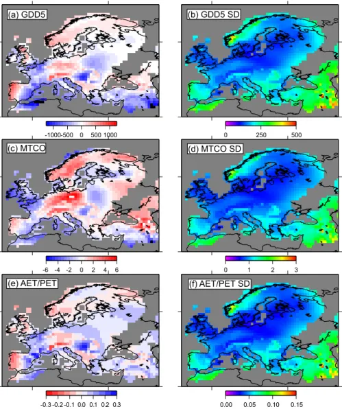
One of the major obstacles in comparing GCM output with site-based climate reconstructions is the question of scale. The values obtained from a model represent single gridboxes, which may each cover hundreds of square kilometres. In contrast, fossil sites represent point data sources with a lim-ited catchment area, varying from less than a kilometre to several tens of kilometres (Jacobson Jr. and Bradshaw, 1981), and may be influenced by local effects that are effectively averaged out within a model gridbox. In order to limit the problems encountered when comparing information at dif-ferent scales, we have used a set of gridded palaeoclimate reconstructions (Davis et al., 2003; Fig. 1).
A comparison of the data and model output for the mid-Holocene shows a large difference between the ranges of reconstructed changes and simulated changes (Fig. 2). As the goal of this study is to compare patterns of change, we have standardised each model output to the overall simulated changes within the region, and the observed changes are stan-dardised to the overall observed pattern. This is intended to provide a method of comparing relative changes, without this being obscured by differences in the magnitude of change. For example, if the region of greatest warming in both model and data occurs in the same region, then this is considered as a good result, even if the magnitude of that warming dif-fers between simulation and observation. We also retain the ratio between the range of simulated and observed changed for each model as a further measure to assess the fit between data and model (the SD ratio).
2 Methods and data
2.1 Study area
In order to be based on a relatively high density of proxy sites, the comparison have been made using pollen-based re-constructions and model grid cells covering the western Eu-ropean continent between 15◦ West and 50◦ East and
be-tween 30◦and 75◦North.
2.2 Proxy data
A data set of palaeo-climate reconstructions for the European continent was used, taken from the recent study based on
-1000-500 0 500 1000 0 250 500 -6 -4 -2 0 2 4 6 0 1 2 3 -0.3 -0.2 -0.1 0.0 0.1 0.2 0.3 0.00 0.05 0.10 0.15 (a) GDD5 (b) GDD5 SD (f) AET/PET SD (d) MTCO SD (e) AET/PET (c) MTCO
Fig. 1. Maps showing the distribution of reconstructed anomalies and the standard deviation of the reconstruction: (a) Growing Degree Days
Over 5◦C (GDD5); (b) GDD5 standard deviation; (c) Mean temperature of the coldest month (MTCO); (d) MTCO standard deviation; (e)
Actual evapotranspiration/potential evapotranspiration (AET/PET); (f) AET/PET standard deviation.
over 400 sites by Davis et al. (2003). These are gridded cli-matic and bioclicli-matic estimates on a regular one degree grid across most of the western European continent (Fig. 1). As the aim of this comparison is to compare climatic changes, 6 ka BP anomalies were calculated by subtracting the recon-structed modern value for each data grid point from the mid-Holocene value. The final dataset included 1505 data grid points. We have selected the three bioclimatic parameters that are the best reconstructed from fossil pollen assemblages for the comparison (moisture availability (AET/PET), tem-perature of the coldest month (MTCO) and growing degree days (GDD5)). These are also the same parameters used in previous comparison studies.
2.3 Models
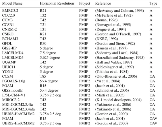
The study includes output from a total of 25 GCMs, com-prised of 14 atmosphere-only GCMs, 9 coupled OAGCMs and 2 coupled OAVGCMs. Details of each model and refer-ences are given in Table 1.
2.4 Summary of method
As the method is fairly complex, a short summary is given here, followed by greater detail concerning each part. The overall aim is to identify regions of homogenous climate changes in the proxy data and then to identify regions in the model output that have similar characteristics. These regions of homogenous climate changes are obtained using cluster analysis of the proxy data, giving a set of “data clusters”,
Table 1. GCMs included in the comparison study. Note that this does not include all models available in the PMIP projects, only those for which all necessary information was available. Type: A – atmosphere only; OA – coupled atmosphere; OAV – coupled ocean-atmosphere-vegetation. For coupled models, the resolution is given for the atmospheric component.
Model Name Horizontal Resolution Project Reference Type
BMRC3.2 R21 PMIP (McAvaney and Colman, 1993) A
CCC2.0 T32 PMIP (McFarlene et al., 1992) A
CCM3 T42 PMIP (Bonan, 1996) A
CCSR1 T21 PMIP (Numagati et al., 1995) A
CNRM-2 T31 PMIP (Deque et al., 1994) A
CSIRO R21 PMIP (Gordon and O’Farrell, 1997) A
ECHAM3 T42 PMIP (DKRZ, 1992) A
GFDL R30 PMIP (Gordon and Stern, 1982) A
GISS-IIP 5 degree PMIP (Hansen et al., 1997) A
LMCELMD4 7.5 degree PMIP (Sadourny and Laval, 1984) A
LMCELMD5 5.625 degree PMIP (Harzallah and Sadourny, 1995) A
UGAMP T42 PMIP (Hall and Valdes, 1997) A
UIUC11 5 degree PMIP (Schlesinger et al., 1997) A
YONU 5 degree PMIP (Tokioka et al., 1984) A
CCSM T85 PMIP2 (Otto-Bliesner et al., 2006) OA
FGOALS-1.0g 5×4 degree PMIP2 (Yu et al., 2004) OA
FOAM R15 PMIP2 (Jacob et al., 2001) OA
GISSmodelE 5×4 degree PMIP2 (Schmidt et al., 2006) OA
IPSL-CM4-V1 3.75×2.5 deg PMIP2 (Marti et al., 2005) OA
MIROC3.2 T42 PMIP2 (K-1 model developers, 2004) OA
MRI-CGCM2.3.4fa T42 PMIP2 (Yukimoto et al., 2006) OA
MRI-CGCM2.3.4nfa T42 PMIP2 (Yukimoto et al., 2006) OA
UBRIS-HadCM3M2 3.75×2.5 deg PMIP2 (Gordon et al., 2000) OA
FOAM R15 PMIP2 (Jacob et al., 2001) OAV
UBRIS-HadCM3M2 3.75×2.5 deg PMIP2 (Gordon et al., 2000) OAV
each containing a number of individual proxy data points with similar direction and magnitude of change in the cli-mate parameters.
On the basis of the simulated changes in the same parame-ters, each model grid box is assigned to the most similar data cluster. The similarity is assessed by measuring the distance in climate space between the data cluster and the model grid box. This distance is measured using a fuzzy distance mea-sure (Bardossy and Duckstein, 1995), which takes into ac-count the uncertainties on both the data and the model. In addition, by accumulating the distances between the model and the data, a general estimate of the “fit” between data and model may be obtained.
Once the gridboxes of a model have been assigned to the clusters, a set of comparison statistics are calculated. These include:
a) the median climate distance between the data clusters and the model. This measure allows an assessment of how well the model reproduces the value of the recon-structed changes, and is location independent.
b) the median geographical distance between the location of each model grid box and its associated data cluster.
This allows an assessment of how closely situated each model grid box is to its associated data cluster.
c) the number of clusters found in the model. This is used to assess whether the model simulates the same types of changes found in the reconstruction.
d) the ratio between the magnitude of reconstructed and simulated climate changes.
2.5 K-means cluster analysis
The aim of the cluster analysis is to group together data points showing similar sign and amplitude of climate change. The clusters obtained therefore represent regions in which the change in climate at the mid-Holocene was internally similar. The clusters are defined on the available bioclimatic variables (GDD5, MTCO, AET/PET) and the geographical coordinates of each grid point. The inclusion of the coor-dinates ensures that the clusters are spatially coherent; this facilitates visual comparison between the models and data and is used in comparing the spatial distance between the model gridbox and the data cluster. Here, the cluster analysis
MTCO °C D e n si ty 6 4 2 0 2 4 6 8 0 .0 0 .1 0 .2 0 .3 0 .4
Fig. 2. Distribution of changes in MTCO from the European region obtained from the gridded palaeoclimate reconstructions (blue) and all available simulations (red).
is applied to a matrix consisting of a set of 1505 vectors (one per gridpoint of the reconstructions) by 5 variables.
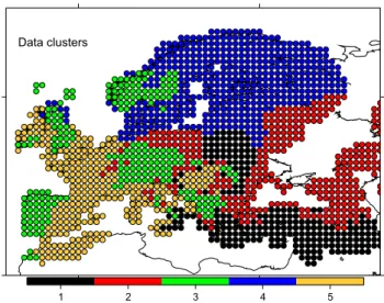
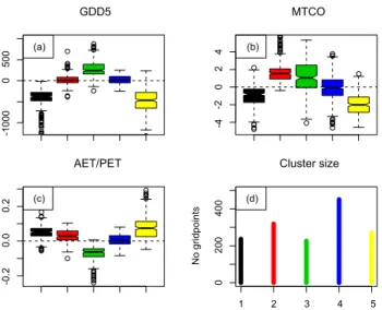
The k-means algorithm was used for cluster analysis (Har-tigan and Wong, 1979). The number of groups to be obtained is a priori unknown, and the choice is somewhat arbitrary. In order to select an optimum number, we use the ratio of inter to intra-group variance of an increasing number of groups, and consider a stopping rule when the gain was less than 0.05, resulting in the selection of five groups. Each group can be characterised by its centroid or centre of gravity, the average point in the multidimensional space defined by the variables. We then test to see if a different set of groups may be obtained if a different random start is used by examining a) if other possible sets of centroids may be obtained; and b) the amount by which the centroids of these groups vary. The k-means algorithm was run 1000 times using a different ran-dom start each time, and the standard deviation of the value attributed to the centroid was calculated. A low value means that the centroids do not vary significantly, and the set of five clusters obtained can be considered as stable. The geograph-ical distribution of the selected clusters is shown in Fig. 3. For the comparison, each cluster is represented by its cen-troid and its extent on each climatic axis and Fig. 4 shows the extent of each cluster in terms of these parameters.
2.6 Hagaman distance
Once the clusters have been established, the next step is to assign each model gridbox to one of these clusters, in other words to define which observed pattern of climate changes is simulated for that gridbox. In order to assign individual grid-boxes to the clusters, it is necessary to measure the climatic
1 2 3 4 5
Data clusters
Fig. 3. Map showing the distribution of the 5 climatically defined clusters used in the comparison.
distance between gridbox and cluster. To include information about model and data uncertainties, we have replaced mea-sures based on Euclidean distances with a distance based on fuzzy numbers, the Hagaman distance (Bardossy and Duck-stein, 1995). A fuzzy number is defined by a membership function, which may be defined by a central value, an upper and lower limit around this value and the shape of the func-tion. We have used triangular fuzzy numbers, which make the least assumptions about the distribution of these errors. This is of particular use with proxy errors, which are fre-quently asymmetric and non-Gaussian.
For each climatic parameter i that is used to define the clus-ters, we obtain two triangular numbers (ri, ri−δri, ri+ηri)
and (mi, mi−δmi, mi+ηmi). The first represents the proxy
data cluster, where the position of the triangle apex (ri) is
the cluster centroid and the limits ri−δriand ri+ηri are
de-fined by the 5th and 95th percentile, respectively. The sec-ond triangular fuzzy number represents the model climate at gridpoint i. The apex (mi) is the mean model value at that
point and the limits mi−δmi and mi+ηmi are +/−2 standard
deviations of the interannual variability of that grid-point. A description of the calculation of the Hagaman distance used is given in Brewer et al. (2007). Here, we calculate, for each model gridpoint, the Hagaman distance to each of the five se-lected clusters. For comparison, the model grid-point is then assigned to the closest, and therefore most similar, of the five clusters. We retain a list of the distances to the assigned clus-ters for the comparison step.
2.7 Comparison statistics
Four results are available from the comparison to assess model performance:
-1 0 0 0 0 5 0 0 GDD5 (a) -4 0 2 4 MTCO (b) -0 .2 0 .0 0 .2 AET/PET (c) 1 2 3 4 5 0 2 0 0 4 0 0 Cluster size N o g ri d p o in ts (d) -2
Fig. 4. Climatic characteristics of the 5 clusters, in terms of the three parameters used, given as anomalies from modern values: (a) GDD5; (b) MTCO; (c) AET/PET; (d) cluster size. For each param-eter, the centre line of each box gives the median value, the lower and upper limits of the box represent the 25th and 75th percentile and the lower and upper whisker give the 5th and 95th percentile, respectively. The circles represent outliers with values greater than the 95th percentile or lower than the 5th percentile.
a) the number of clusters reproduced by each model b) the Hagaman distance between the observed and
simu-lated changes
c) the geographical distance between the observed cluster of climate changes and each model grid box.
d) the ratio between the range of mean reconstructed and simulated anomalies (the SD ratio)
The first two of these measures allow an assessment of how closely a model reproduces the observed changes in climate space, i.e. whether that model is simulating similar climatic changes, even if these are spatially displaced and a model that has similar climatic values will have a low distance. From the list of Hagaman distances obtained, the median, 5th and 95th percentiles of the distances obtained are used for model intercomparison. The fit between the spatial pat-tern of the changes is assessed using the third measure (Ta-ble 2 and Fig. 5). This is measured as the Hagaman distance between the location of each model grid box and the cluster to which it is assigned. The comparison is in the same geo-graphical units as the coordinates, i.e. decimal degrees, and there may be some bias due to the difference in longitudi-nal length with increasing latitude. However, this should be negligible within the relatively constrained study area. The SD ratio between the ranges of reconstructed and simulated anomalies is used to assess how well the models simulate the
magnitude of change seen in the proxy data. This is calcu-lated as the ratio of the standard deviation of the simucalcu-lated anomalies to the standard deviation of reconstructed anoma-lies, and is given in Table 2.
Finally, the ability of the model to predict the correct di-rection of mid-Holocene climate changes was tested by com-paring the simulated modern climate with the proxy data (i.e. using zero model anomalies). Table 2 also gives geographi-cal distances to a random assignment of clusters to the model grid boxes and to a perfect fit between model and data.
3 Results
3.1 Description of proxy-based clusters 3.1.1 Cluster 1 (Southeastern cluster)
The first cluster is found in eastern Europe, mainly around the eastern Mediterranean basin and to the south of the Black Sea. It also occurs further north in central eastern Europe. It is characterised by decreased temperatures in both winter and summer, and increased moisture availability.
3.1.2 Cluster 2 (Continental cluster)
Cluster 2 is mainly found in eastern Europe, where it cov-ers a large area of western Russia, down to the Black Sea. It is also found to a lesser extent on the southern coast of the Baltic Sea. This cluster is characterised by increases in temperatures of the coldest month, and slightly wetter condi-tions. This suggests that the seasonal contrast of the climate was reduced.
3.1.3 Cluster 3 (Atlantic cluster)
The third cluster has a non-continuous distribution in west-ern Europe, occurring extensively along the Atlantic coast in the Iberian peninsula, the British Isles and Scandinavia, but also around and to the north of the Alps. The cluster is char-acterised by increases in winter temperatures and GDD5, and drier than present conditions.
3.1.4 Cluster 4 (Northern cluster)
Cluster 4 is found across northern Europe, from Scotland to Finland. Whilst a range of anomalies is found, overall the cluster shows little climatic change from today.
3.1.5 Cluster 5 (Western cluster)
The final cluster is found in the west of Europe, from the western Mediterranean to the south of the British Isles. Cli-matically, it is similar to the first cluster, with cooler tempera-tures and increased moisture availability, and is distinguished by slightly colder winters.
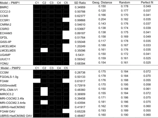
Table 2. Simulated clusters by model. Black squares indicate that the cluster is simulated at least once within the study area. White squares represent clusters that were not found in the simulation. The SD Ratio gives the ratio between the range of observed and simulated changes to assess the amplitude of the modelled climatic variations. The column “Geog Distance” gives the median geographical distance between each model grid point and the location of the centroid to which it has been assigned. This may be used to assess the fit between observed and simulated spatial patterns. The final two columns give the geographical distance when tested against 1000 random distributions of clusters on the model grid, and to a perfect fit. The perfect fit was established by assigning to each model grid box the most common data cluster found within it.
Model – PMIP1 C1 C2 C3 C4 C5 SD Ratio Geog. Distance Random Perfect fit
BMRC 0.34959 0.150 0.178 0.049 CCC2.0 0.50788 0.120 0.177 0.037 CCM3 0.62377 0.166 0.170 0.041 CCSR1 0.99868 0.204 0.182 0.035 CNRM-2 0.54610 0.143 0.176 0.037 CSIRO 0.53667 0.138 0.174 0.039 ECHAM3 0.89187 0.138 0.175 0.041 GFDL 0.51764 0.158 0.169 0.049 GISS-IIP 0.55048 0.117 0.178 0.035 LMCELMD4 1.20249 0.189 0.167 0.033 LMCELMD5 0.35096 0.161 0.176 0.035 UGAMP 0.5431 0.150 0.172 0.041 UIUC11 0.59342 0.159 0.161 0.025 YONU 0.68394 0.154 0.161 0.025 Model – PMIP2 C1 C2 C3 C4 C5 CCSM 0.26738 0.175 0.184 0.072 FGOALS-1.0g 0.50133 0.178 0.184 0.070 FOAM 0.61617 0.176 0.188 0.055 GISSmodelE 0.72919 0.170 0.195 0.058 IPSL-CM4-V1 0.48360 0.150 0.188 0.061 MIROC3.2 0.36909 0.155 0.184 0.072 MRI-CGCM2.3.4fa 0.39458 0.171 0.186 0.075 MRI-CGCM2.3.4nfa 0.43594 0.181 0.186 0.075 UBRIS-HadCM3M2 0.41917 0.162 0.190 0.060 FOAM OAV 0.65228 0.193 0.189 0.055 UBRIS-HadCM3M2 OAV 0.48467 0.160 0.190 0.060
3.2 Description of model-based clusters
The main results of the comparison exercise for the models are summarised in Table 2 and the spatial distribution of the simulated is shown in Fig. 5. These results show that all models are able to simulate the direction of change of four of the five clusters, and 9 PMIP1 models and 7 PMIP2 mod-els are able to simulate the direction of change of all five clusters. Although most simulations appear to show a good agreement with the proxy data, the majority of models are dominated by the Atlantic (3) and Northern (4) clusters. The Northern cluster shows the smallest amount of change from the modern climate, and this result highlights the fact that the models simulate a smaller range of climate changes than those seen in the data. The SD ratio of the observed and simulated changes (i.e. the difference in magnitude) is also given in Table 2 and shows that the magnitude of changes simulated by the models may be as low as one quarter of the observed range, but is generally between 30% and 70% of the reconstructed changes.
3.3 Variance and distances
In order to compare between the different simulations, we have plotted each model as a function of the distances ob-tained between its simulated climate and the proxy clusters, and the SD ratio described above (Fig. 6). The figure shows that the median distance for the mid-Holocene simulation is lower than the modern simulation for all models and the ma-jority of models are grouped together, with a median distance of between 1 and 4 and a SD ratio of between 0.3 and 0.7.
4 Discussion
4.1 Choice of proxy data
One important change in the current study from the previ-ous mid-Holocene data-model comparison is the use of a new proxy dataset. The studies by Masson et al. (1998), Guiot et al. (1999), and Bonfils et al. (2004) all used the set of climate reconstructions of produced by Cheddadi et al. (1997). As there are a number of differences between
(a) BMRC CCC2.0 CCM3 CCSR1 CNRM2 CSIRO ECHAM3 GFDL GISSIIP 1 2 3 4 5 (b)
LMCELMD4 LMCELMD5 UGAMP
UIUC11 YONU
1 2 3 4 5
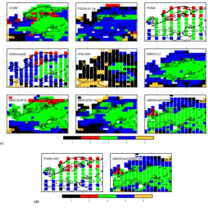
Fig. 5. Geographic distribution of clusters obtained for each model. (a) and (b) PMIP1 models; (c) PMIP2 OA coupled models; (d) PMIP2 OAV coupled models.
this reconstruction, and the estimations of Davis et al. (2003) used in the current study, it is worth briefly describing them and discussing the implications for comparative studies.
The radiocarbon dates used to attribute the pollen sam-ples to the mid-Holocene were uncalibrated in Cheddadi et al. (1997) and calibrated in Davis et al. (2003). There will
(c)
CCSM FGOALS1.0g FOAM
GISSmodelE IPSLCM4 MIROC3.2
MRICGCM fa MRICGCM nfa UBRISHadCM3M2
1 2 3 4 5
(d)
FOAM OAV UBRISHadCM3M2 OAV
1 2 3 4 5
Fig. 5. Continued.
therefore have been a difference in the fossil samples chosen to represent 6000 years BP. As no rapid or marked changes in mean climate or vegetation have been reported for this pe-riod, it is unlikely that this will have had a large effect on the reconstructed climate values. Both studies used a modern analogue technique to reconstruct climate, but with different constraining factors. The use of lake-levels as a constraint in the Cheddadi et al study in particular appears to have re-duced the amount of noise in the reconstructions. In their paper, Davis et al. (2003) compared their mid-Holocene re-sults with those of Cheddadi et al, and noted that both studies showed a similar spatial structure with a generally warmer
north and generally cooler south. This suggests that the di-rections of climate change that are used to test the models have not changed, but the magnitude of those changes may be amplified in the Davis et al dataset. We have chosen to keep the dataset as it is attributed to the correct time period, but the interpretation of the SD ratios presented above, must be made with care.
A recent study based on proxy data and the PMIP2 simu-lations has suggested that the mid-Holocene may have been characterised by positive NAO-like shift in the mean climate (Gladstone et al., 2005). This is supported by the observed pattern of changes in temperatures with warming in the north,
0.2 0.4 0.6 0.8 1.0 0 2 4 6 8 1 0 1 2 SD Ratio D ist a n ce PMIP1 PMIP1 ZERO PMIP2 PMIP2 ZERO BMRC CCC2.0 GISSIIP GISSmodelE MRICGCM2.3.4fa IPSL YONU CCSM LMCELMD5 FOAMoa FOAMoav MRICGCM2.3.4nfa UBRISHadCM3M2oav ECHAM CCSR1 UIUC11 CCM3 CNRM2 YGAMP GFDL MIROC3.2 UBRISHadCM3M2oa CSIRO FGOALS1.0 Model-model comparison
Fig. 6. Results of final comparison. Each model is represented by a bar describing the range of Hagaman distances obtained. The limits of the bar are the 5th and 95th percentile and the median distance is shown by a closed symbol. The open symbols are the results of the comparison using zero anomalies, i.e. the modern simulated climate. The position of the bars on the x-axis represents the ratio between the range of simulated and observed values. On this figure, a model with a perfect fit to the data would have a distance of zero and a ratio of values of 1, and is indicated by a green star.
but the increased humidity in the south appears more related to an increase in precipitation over the Mediterranean basin, resulting from an increase in advection of humidity from the Atlantic (Bonfils et al., 2004)
4.2 Comparison data-model
The clusters obtained for each model are summarised in Ta-ble 2 and Fig. 5. These results show that although the same patterns of change are reproduced in nearly all the models, the spatial distribution of these changes varies widely. In to-tal, 15 models simulate all five climate patterns represented by the clusters in at least one gridbox. Three of the identified patterns of climate change are consistently reproduced, and these show quite contrasting sets of changes (the cool and wet Southeastern cluster, the warm and dry Atlantic cluster and the “zero anomaly” Northern clusters). The models are therefore able to simulate complex patterns of change within a relatively restricted geographical area.
Clusters 1 and 5 represent the cooler and wetter climate of southern Europe during the mid-Holocene. Previous data-model comparison studies have shown that this climate pat-tern is rarely simulated for the mid-Holocene over Europe (Masson et al., 1998; Bonfils et al., 2004), as the increased summer insolation forces an increase in GDD5 (Masson et al., 1998). A decrease in growing season length and intensity may, however, be controlled by a reduction in winter tem-peratures and increased summer evapotranspiration (Bonfils, 2001). The results of the tests obtained here suggest that the
models are able to simulate this pattern of climate changes, although the fifth cluster (the Western cluster) is frequently missing. This is perhaps unsurprising, as the changes in this region are more extreme than in the Southeastern clus-ter (Fig. 4), and the simulated changes are generally smaller than the observed changes. The only exception is the FOAM-OA GCM, which fails to simulate either of the two Mediter-ranean clusters (1 and 5).
The second (Continental) and third (Atlantic) clusters both show an increase in winter temperature and drier than present conditions. The Atlantic cluster, which is simulated by all models, also shows an increase in GDD5, in response to the increased summer insolation, a dominant forcing factor in the simulations (Joussaume et al., 1999). However, the increase in winter temperatures is more surprising, as win-ter insolation was lower during the mid-Holocene than today (Berger, 1978). Bonfils (2001) suggests that heating from hu-midity advection would have dominated the relatively weak decrease in insolation at high latitudes. In the Continental cluster, there is no increase in GDD5. In this region, any potential GDD5 increase due to higher summer temperatures is limited by a loss of energy with increased summer evapo-transpiration.
A visual comparison of the spatial distribution of the proxy clusters and the simulated clusters shows a number of differ-ences between the data and models and between the different models. A number of models show the first (Southeastern) cluster in the same location as the observed pattern (CCC2.0, CCM3, CNRM2, GISS-IIP, UGAMP, FGOALS, IPSL-CM4-V1-MR, MIROC3.2, MRI-2.3.4fa). However, the simulated cluster is frequently more widespread, particularly toward the western Mediterranean. The IPSL-CM4-V1-MR model, which is characterised by colder temperatures, is dominated by this cluster. The second (Continental) cluster is correctly located in a number of PMIP1 models (BMRC, CNRM2, GFDL, GISS-IIP). When found in other models, it is fre-quently shifted to the north, notably in the PMIP2 models. The increased advection of warm, moist oceanic air in win-ter that results in these changes (wetwin-ter conditions, warmer winters and little change in GDD5) therefore appears to be simulated further north than in the observations. This is in agreement with Masson-Delmotte et al. (2006), who found in a data-model comparison in polar regions that changes in moisture advection were not correctly simulated. The warm and dry third cluster (Atlantic) is frequently widespread in the simulations. While it therefore occurs in the same loca-tion as the observaloca-tions in nearly all models, the simulated distribution generally extend further to the east than the ob-servations. The “zero anomaly” cluster (4) has a wide distri-bution in a number of simulations. However, it is correctly simulated in the north of Europe by several models (CCC2.0, CCM3, CSIRO, UGAMP, UIUC11, YONU, FGOALS, GISS-IIP, MIROC3.2, MRI2.3.4nfa, UBRIS-HadCM3M2-oa and UBRIS-HadCM3M2-UBRIS-HadCM3M2-oav).
in a few models (BMRC, UGAMP, PSL-CM4-V1-MR and MIROC3.2). A number of other PMIP2 models simulate this cluster in the southwest of Europe, but to the south of its loca-tion in the observaloca-tions, suggesting that a cooling of greater intensity occurs in the PMIP2 simulations, but is shifted to the south. Overall, the occurrence of the two cooler and wet-ter cluswet-ters in the PMIP2 models suggests that they simulate more successfully the pattern of climate change in southern Europe than the previous models.
An estimation of the average distance between the model gridboxes and their assigned clusters is also given in Table 2. On the basis of this and the SD ratio between observed and simulated changes, there is no clear “better” model. Some models (e.g. CCSR1 and LMCELMD4) have high SD ratios, but have high geographical distances, suggesting that whilst the simulated values are similar to the observed ones, their spatial distribution does not resemble the observed pattern. Other models (CCC2.0 and GISS-IIP) have low geographi-cal distances, suggesting that the spatial patterns are similar to the observed patterns, but do only simulate half the am-plitude of the observed changes. The PMIP2 models geo-graphical distances are generally higher, suggesting that the simulated pattern from the coupled models differ more from the observed patterns. Of all the models tested, GISS-IIP has the spatial structure closest to that of the data, with only cluster 5 displaced to the east.
4.3 Model-model
In order to compare the simulations between the different models, we have plotted the range of Hagaman distances obtained against the SD ratio of anomalies (Fig. 6). This shows that the majority of models have similar results and are grouped together, with a median distance of between 1 and 4 and a SD ratio of between 0.3 and 0.7. No obvious dis-tinction can be made between the PMIP1 and PMIP2 mod-els, suggesting that despite the increase in model complexity, there is no clear change in simulation results. This is perhaps a little surprising, as the PMIP2 models show a better ability to reproduce the problematic cool and wet cluster 5 (West-ern), however models that best reproduce this cluster (e.g. IPSL-CM4-V1-MR and MIROC3.2) have less success in re-producing the warm and dry patterns (clusters 1 and 5). An exception to this is the PMIP2 model GISSmodelE, which has a gradient of GDD5 anomalies over Europe that are very similar to those observed in the data, and thus reproduces the cooler south and warmer north. Of the models that fall outside of this group, one (CCSM) has a low SD ratio of anomalies and a relatively poor fit. The changes simulated are relatively small, when compared to the other models, and the low fit may result in part from a reduced interannual vari-ability. Three PMIP1 models are distinguished by high SD ratios of anomalies (ECHAM3, CCSR1 and LMCELMD4).
tably, have much higher interannual variability.
Simulations were available from a flux-adjusted and non-flux-adjusted version of one PMIP2 model, the OAGCM from the Japanese Meteorological Research Institute (respec-tively MRI-CGCM2.3.4fa and MRI-CGCM2.3.4nfa). Both versions of the model have a similar median Hagaman dis-tance, suggesting the removal of flux-adjustment does not affect the general ability of this model to simulate the mid-Holocene climate of Europe. The non-flux-adjusted version does have a much larger range of Hagaman distances, due mainly to a greater winter cooling in the north of Europe in this version of the model, and the Continental cluster (2), characterised by warmer winters, is not simulated in this ver-sion of the model.
Two models were available from the PMIP2 project as coupled OAGCMs and fully coupled OAVGCMs (FOAM, UBRIS-HadCM3M2). In both cases, the inclusion of a cou-pled vegetation model improves the output by increasing the range of anomalies simulated, thus giving an output closer to the data values. Whilst little difference can be seen between the two UBRIS-HadCM3M2 simulations, the fully coupled FOAM model shows an improved fit to the observations. The fully coupled version of the FOAM model shows signs of a greater cooling in the south as the warm, dry cluster 3 is replaced by the “zero anomaly” cluster across the Mediter-ranean basin. In addition, one of the cool, wet clusters (clus-ter 1) is reproduced, albeit only within one grid box. This cooling is related to a better representation of vegetation, par-ticularly over the Sahara and underlines the importance of in-cluding interactive vegetation. There is, however, no obvious difference between the fully coupled OAVGCM simulations and the main group of simulations on Fig. 6.
Finally, the test against zero anomalies (ZERO, Fig. 6) shows a higher median Hagaman distance than for the mid-Holocene simulation for all models. This indicates that in all cases, the simulated change under the mid-Holocene forcing follows the same direction of change as the data, and repre-sents an improvement over the modern climatology.
5 Conclusions
We have used climate reconstructions from a dataset of fos-sil pollen sites to test to ability of a group of climate models of varying complexity to simulate the changes of the mid-Holocene climate over Europe. Using three climatic param-eters, five patterns of climatic changes were identified in the data, ranging from cooler and wetter than present to warmer and drier. A fuzzy logic approach was used to assign the model simulations to these clusters, allowing the identifica-tion of the patterns that are simulated by each model, and the geographic distribution of these patterns. Four comparison statistics were calculated, allowing a comparison to be made
of the amplitude and sign of climate changes simulated and the spatial pattern of these changes.
The results show that, although the models are not able to simulate the magnitude of the climate changes reconstructed in the pollen, they perform well in capturing the different pat-terns of change, with four of the five patpat-terns reproduced in the majority of models. Little distinction is shown between the first generation of atmosphere-only models and the newer coupled atmosphere-ocean models. In contrast, comparisons between different runs of the same model, with either differ-ent levels of complexity (FOAM, UBRIS-HadCM3M2) or removal of flux-adjustment, show improvements in the range of values reconstructed. Further, the new generation PMIP2 models reproduce more successfully the pattern of cooler and wetter climate change in southern Europe than the previous models.
Despite their low spatial resolution, the models are capa-ble of reproducing the quite complicated directions of change observed in a relatively restricted geographical area. There remains a problem with the size of the simulated changes that are lower than those observed, although this is, in part, related to noise in the proxy reconstructions. Further, the spatial pattern of the simulated changes is frequently dif-ferent from the data. In the region considered, the climatic changes for the mid-Holocene are relatively slight. Further work will apply these methods to larger regions for which data are available, e.g. the northern Hemisphere or to areas where large-scale changes in the climate have been observed, e.g. the African monsoon (Joussaume et al., 1999; Braconnot et al., 2000; Bonfils et al., 2001).
Acknowledgements. We thank three anonymous reviewers and
N. Weber for comments and criticism that have improved both the analysis and the scope of this paper. We acknowledge the interna-tional modeling groups for providing their data for analysis, the Laboratoire des Sciences du Climat et de l’Environnement (LSCE) for collecting and archiving the model data, and we thank P. Bra-connot for helpful discussion on the method and its application. The PMIP2/MOTIF Data Archive is supported by CEA, CNRS, the EU project MOTIF (EVK2-CT-2002-00153) and the Programme National d’Etude de la Dynamique du Climat (PNEDC). The analyses were performed using version 11-20-2005 of the database. More information is available on http://www-lsce.cea.fr/pmip/ and http://www-lsce.cea.fr/motif/.
Edited by: N. Weber
References
Bardossy, A. and Duckstein, L.: Fuzzy Rule-Based Modelling with Applications to Geophysical, Biological, and Engineering Sys-tems, CRC Press, Boca Raton, Florida, 1995.
Berger, A. L.: Long-term variations of daily insolation and Quater-nary climatic changes, J. Atmos. Sci., 35(12), 2362–2367, 1978. Bonan, G. B.: A land surface model (LSM version 1.0) for ecologi-cal, hydrologiecologi-cal, and atmospheric studies: technical description
and user’s guide, NCAR/TN-417+STR, NCAR, Boulder, CO, 1996.
Bonfils, C.: Le moyen-Holoc`ene: rˆole de la surface continentale sur la sensibilit´e climatique simul´ee, PhD Thesis, Universit´e Paris VI, Paris, 322 pp., 2001.
Bonfils, C., de Noblet-Ducoudre, N., Braconnot, P., and Joussaume, S.: Hot desert albedo and climate change: Mid-Holocene mon-soon in North Africa, J. Climate, 17, 3724–3737, 2001. Bonfils, C., de Noblet-Ducoudre, N., Guiot, J., and Bartlein, P.:
Some mechanisms of mid-Holocene climate change in Europe, inferred from comparing PMIP models to data, Clim. Dynam., 23, 79–98, 2004.
Braconnot, P. and Frankignoul, C.: Testing model simulations of the thermocline depth variability in the tropical Atlantic from 1982 through 1984, J. Phys. Oceanogr., 23, 626–647, 1993.
Braconnot, P., Joussaume, S., de Noblet, N., and Ramstein, G.: Mid-Holocene and last glacial maximum African monsoon changes as simulated within the Paleoclimate Modeling Inter-comparison Project, Global Planet. Change, 26, 51–66, 2000. Braconnot, P., Otto-Bliesner, B., Harrison, S., Joussaume, S.,
Pe-terschmitt, J. Y., Abe-Ouchi, A., Crucifix, M., Fichefert, T., He-witt, C. D., Kageyama, M., Kitoh, A., Loutre, M. F., Marti, O., Merkel, U., Ramstein, G., Valdes, P., Weber, S. L., Yu, Y., and Zhao, Y.: Results of PMIP2 coupled simulations of the Mid-Holocene and Last Glacial Maximum – Part 1: experiments and large-scale features, Clim. Past, 3, 261–277, 2007,
http://www.clim-past.net/3/261/2007/.
Brewer, S., Alleaume, S., Guiot, J., and Nicault, A.: Historical droughts in Mediterranean regions during the last 500 years: a data/model approach, Clim. Past, 3, 355–366, 2007,
http://www.clim-past.net/3/355/2007/.
Cheddadi, R., Yu, G., Guiot, J., Harrison, S. P., and Prentice, I. C.: The climate of Europe 6000 years ago, Clim. Dynam., 13, 1–9, 1997.
Davis, B. A. S., Brewer, S., Stevenson, A. C., Guiot, J., and Data Contributors: The temperature of Europe during the Holocene reconstructed from pollen data, Quaternary Sci. Rev., 22, 1701– 1716, 2003.
Deque, M., Dreveton, C., Braun, A., and Cariolle, D.: The
ARPEGE/IFS atmosphere model: A contribution to the French community climate modelling, Clim. Dynam., 10(4/5), 249–266, 1994.
Deutsches Klimarechenzentrum (DKRZ) Modellbetreuungsgruppe: The ECHAM3 atmospheric general circulation model, DKRZ Tech. Report No. 6, DKRZ, Hamburg, 1992.
Gladstone, R. M., Ross, I., Valdes, P. J., Abe-Ouchi, A., Braconnot, P., Brewer, S., Kageyama, M., Kitoh, A., Legrande, A., Marti, O., Ohgaito, R., Otto-Bliesner, B., Peltier, W. R., and Vettoretti, G.: Mid-Holocene NAO: a PMIP2 model intercomparison, Geophys. Res. Lett., 32, 16 707, doi:10.1029/2005GL023596, 2005. Gordon, C., Cooper, C., Senior, C. A., Banks, H., Gregory, J. M.,
Johns, T. C., Mitchell, J. F. B., and Wood, R. A.: The simulation of SST, sea ice extents and ocean heat transports in a version of the Hadley Centre coupled model without flux adjustments, Clim. Dynam., 16, 147–168, 2000.
Gordon, C. T. and Stern, W. F.: A description of the GFDL global spectral model, Mon. Wea. Rev., 110, 625–644, 1982.
Gordon, H. B. and O’Farrell, S. P.: Transient Climate Change in the CSIRO Coupled Model with Dynamic Sea Ice, Mon. Wea. Rev.,
Guiot, J., Boreux, J. J., Braconnot, P., Torre, F., and PMIP par-ticipating groups: Data-model comparisons using fuzzy logic in palaeoclimatology, Clim. Dynam., 15, 569–581, 1999.
Hall, N. M. J. and Valdes, P. J.: A GCM simulation of the climate 6000 years ago, J. Climate, 10, 3–17, 1997.
Hansen, J. E., Sato, M., Ruedy, R., Lacis, A. A., Asamoah, K., Beckford, K., Borenstein, S., Brown, E., Cairns, B., Carlson, B., Curran, B., de Castro, S., Druyan, L., Etwarrow, P., Ferede, T., Fox, M., Gaffen, D., Glascoe, J., Gordon, H. B., Hollandsworth, S., Jiang, X., Johnson, C., Lawrence, N., Lean, J., Lerner, J., Lo, K. K., Logan, J., Luckett, A., McCormick, M. P., McPeters, R., Miller, R. L., Minnis, P., Ramberran, I., Russell, G., Russel, P., Stone, P. H., Tegen, I., Thomas, S., Thomason, L., Thompson, A., Wilder, J., Willson, R., and Zawodny, J.: Forcings and chaos in interannual to decadal climate change, J. Geophys. Res., 102, 25 679–25 720, 1997.
Harrison, S. P., Jolly, D., Laarif, F., Abe-Ouchi, A., Herterich, K., Hewitt, C., Joussaume, S., Kutzbach, J. E., Mitchell, J., Noblet, N. D., and Valdes, P.: Intercomparison of simulated global veg-etation distributions in response to 6kyr BP orbital forcing, J. Climate, 11, 2721–2742, 1998.
Hartigan, J. A. and Wong, M. A.: A K-means clustering algorithm, Appl. Stat., 28, 100–108, 1979.
Harzallah, A. and Sadourny, R.: Internal versus SST-forced atmo-spheric variability as simulated by an atmoatmo-spheric general circu-lation model, J. Climate, 8, 474–495, 1995.
Jacob, R., Schafer, C., Foster, I. D. L., Tobis, M., and Andersen, J.: Computational design and performance of the fast ocean atmo-sphere model: version 1, Proc. 2001 International Conference on Computational Science, Springer-Verlag, 175–184, 2001. Jacobson Jr., G. L. and Bradshaw, R. H. W.: The selection of
sites for palaeovegetational studies, Quaternary Res., 16, 80–96, 1981.
Joussaume, S. and Taylor, K.: Status of the Paleoclimate Modeling Intercomparison Project (PMIP), 92, 425–430, 1995.
Joussaume, S., Taylor, K. E., Braconnot, P., Mitchell, J. F. B., Kutzbach, J. E., Harrison, S. P., Prentice, I. C., Broccoli, A. J., Abe-Ouchi, A., Bartlein, P. J., Bonfils, C., Dong, B., Guiot, J., Herterich, K., Hewitt, C. D., Jolly, D., Kim, J. W., Kislov, A., Kitoh, A., Loutre, M. F., Masson, V., McAvaney, B., McFarlane, N., de Noblet, N., Peltier, W. R., Peterschmitt, J. Y., Pollard, D., Rind, D., Royer, J. F., Schlesinger, M. E., Syktus, J., Thomp-son, S., Valdes, P., Vettoretti, G., Webb, R. S., and Wyputta, U.: Monsoon changes for 6000 years ago: results of 18 simula-tions from the Paleoclimate Modeliing Intercomparison Project (PMIP), Geophys. Res. Lett., 26(7), 859–862, 1999.
K-1 model developers: K-1 coupled model (MIROC) description, K-1 technical report 1, Center for Climate System Research, Uni-versity of Tokyo.
Kim, J.-H. and Schneider, R. R.: GHOST global database for alkenone-derived Holocene sea-surface temperature records, 2004.
Liao, X., Street-Perrott, F., and Mitchell, J.: GCM experiments with different cloud parameterization: comparisons with palaeocli-matic reconstructions for 6000 years BP, Data Model., 1, 99–123, 1994.
Marti, O., Braconnot, P., Bellier, J., Benshila, R., Bony, S., Brock-mann, P., Cadulle, P., Caubel, A., Denvil, S., Dufresne, J. L.,
Grandpeix, J.-Y., Hourdin, F., Krinner, G., L´evy, C., Musat, I., Talandier, C., and the IPSL Global Climate Modeling Group: The new IPSL climate system model: IPSL-CM4, IPSL, Paris, 2005.
Masson, V., Cheddadi, R., Braconnot, P., Joussaume, S., Texier, D., and Participants, P.: Mid-Holocene climate in Europe: what can we infer from PMIP model-data comparisons?, Clim. Dynam., 15, 163–182, 1998.
Masson-Delmotte, V., Kageyama, M., Braconnot, P., Charbit, S., Krinner, G., Ritz, C., Guilyardi, E., Jouzel, J., Abe-Ouchi, A., Crucifix, M., Gladstone, R. M., Hewitt, C. D., Kitoh, A., LeGrande, A. N., Marti, O., Merkel, U., Motoi, T., Ohgaito, R., Otto-Bliesner, B., Peltier, W. R., Ross, I., Valdes, P. J., Vettoretti, G., Weber, S. L., Wolk, F., and Yu, Y.: Past and future polar am-plification of climate change: climate model intercomparisons and ice-core constraints, Clim. Dynam., 26, 513–529, 2006. McAvaney, B. J. and Colman, R. A.: The BMRC Model: AMIP
configuration, BMRC Research Report 38, Melbourne, 1993. McFarlene, N. A., Boer, G. J., Blanchet, J.-P., and Lazare, M.: The
Canadian Climate Centre Second-Generation General Circula-tion Model and its equilibrium climate, J. Climate, 5, 1013–1044, 1992.
Numagati, A., Takahashi, M., Nakajima, T., and Sumi, A.: Devel-opment of an atmospheric general circulation model, in: Climate System Dynamics and Modelling, edited by: Matsuno, T., Uni-versity of Tokyo, Tokyo, 1–27, 1995.
Otto-Bliesner, B., Brady, E. C., Clauzet, G., Tomas, R., Levis, S., and Kothavala, Z.: Last Glacial Maximum and Holocene climate in CCSM3, J. Climate, 19, 2526–2544, 2006.
Prentice, I. C., Harrison, S., Jolly, D., and Guiot, J.: The climate and biomes of europe at 6000 yr BP: comparison of model sim-ulations and pollen-based reconstructions, Quaternary Sci. Rev., 17, 659–668, 1998.
Prentice, I. C., Jolly, D., and Participants, B.: Mid-Holocene and glacial-maximum vegetation geography of the northern conti-nents and Africa, J. Biogeogr., 27, 507–519, 2000.
Sadourny, R. and Laval, K.: January and July performance of the LMD general circulation model, in: New Perspectives in Cli-mate Modelling, edited by: Berger, A. L. and Nicolis, C., Devel-opments in Atmospheric Science, 16, Elsevier, 173–198, 1984. Schlesinger, M. E., Andronova, N. G., Entwhistle, B., Ghanem, A.,
Ramankutty, N., Wang, W., and Yang, F.: Modeling and Simu-lation of Climate and Climate Change, in: Past and present vari-ability of the solar-terrestrial system: Measurements, data anal-ysis and theoretical models, in: Proceedings of the International School of Physics “Enrico Fermi”, edited by: Cini Castagnoli, G. and Provenzale, A., Course CXXXIII. IOS Press, Amsterdam, Varrena, Italy, 389–429, 1997.
Schmidt, G. A., Ruedy, R., Hansen, J. E., Aleinov, I., Bell, N., Bauer, M., Bauer, S., Cairns, B., Canuto, V., Cheng, Y., Del De-nio, A., Faluvegi, G., Friend, A. D., Hall, T. M., Hu, Y., Kelly, M., Kiang, N. Y., Koch, D., Lacis, A. A., Lerner, J., Lo, K. K., Miller, R. L., Nazarenko, L., Oinas, V., Perlwitz, J., Perlwitz, J., Rind, D., Romanou, A., Russell, G. L., Sato, M., Shindell, D. T., Stone, P .H., Sun, S., Tausnev, N., Thresher, D., and Yao, M.-S.: Present day atmospheric simulations using GISS ModelE: Com-parison to in-situ, satellite and reanalysis data, J. Climate, 19, 153–192, 2006.
Texier, D., de Noblet, N., Harrison, S., Haxeltine, A., Jolly, D., Laarif, F., Prentice, I. C., and Tarasov, P.: Quantifying the role of biosphere-atmosphere feedbacks in climate change: coupled model simulations for 6000 years BP and comparison with pa-leodata for northern Eurasia and northern Africa, Clim. Dynam., 13, 865–882, 1997.
Tokioka, T., Yamazaki, K., Yagai, I., and Kitoh, A.: A description of the Meteorological Research Institute atmospheric general cir-culation model (MRI GCM-I), MRI Tech. Report No. 13, Mete-orological Research Institute, Ibaraki-ken, Japan, 1984. Wright Jr., H. E., Kutzbach, J. E., Webb III, T., Ruddiman, W. F.,
Street-Perrott, F., and Bartlein, P. J. (Eds.): Global Climates since the Last Glacial Maximum, University of Minnesota, Minnesota, 544 pp., 1993.
Yu, Y., Zhang, X., and Guo, Y.: Global coupled ocean-atmosphere general circulation models in LASG/IAP, Adv. Atmos. Sci., 21, 444–455, 2004.
Yukimoto, S., Noda, A., Kitoh, A., Hosaka, M., Yoshimura, H., Uchiyama, T., Shibata, K., Arakawa, O., and Kusunoki, S.: Present-day climate and climate sensitivity in the Meteorological Research Institute coupled GCM version 2.3 (MRI-CGCM2.3), J. Meteorol. Soc. Jap., 84, 333–363, 2006.