HAL Id: hal-03206182
https://hal.archives-ouvertes.fr/hal-03206182
Submitted on 15 May 2021
HAL is a multi-disciplinary open access
archive for the deposit and dissemination of
sci-entific research documents, whether they are
pub-lished or not. The documents may come from
teaching and research institutions in France or
abroad, or from public or private research centers.
L’archive ouverte pluridisciplinaire HAL, est
destinée au dépôt et à la diffusion de documents
scientifiques de niveau recherche, publiés ou non,
émanant des établissements d’enseignement et de
recherche français ou étrangers, des laboratoires
publics ou privés.
Distributed under a Creative Commons Attribution - NoDerivatives| 4.0 International
Christopher Hayes, Kassandra Costa, Robert Anderson, Eva Calvo, Zanna
Chase, Ludmila Demina, Jean-claude Dutay, Christopher German, Lars-Eric
Heimbürger, Samuel Jaccard, et al.
To cite this version:
Christopher Hayes, Kassandra Costa, Robert Anderson, Eva Calvo, Zanna Chase, et al.. Global Ocean
Sediment Composition and Burial Flux in the Deep Sea. Global Biogeochemical Cycles, American
Geophysical Union, 2021, �10.1029/2020GB006769�. �hal-03206182�
1. Introduction
Seafloor sediments contain information about many large-scale processes in the ocean such as surface bi-ological productivity, particle export and degradation, hydrothermal activity, and material transport from
Abstract
Quantitative knowledge about the burial of sedimentary components at the seafloor has wide-ranging implications in ocean science, from global climate to continental weathering. The use of230Th-normalized fluxes reduces uncertainties that many prior studies faced by accounting for the effects
of sediment redistribution by bottom currents and minimizing the impact of age model uncertainty. Here we employ a recently compiled global data set of 230Th-normalized fluxes with an updated database of
seafloor surface sediment composition to derive atlases of the deep-sea burial flux of calcium carbonate, biogenic opal, total organic carbon (TOC), nonbiogenic material, iron, mercury, and excess barium (Baxs).
The spatial patterns of major component burial are mainly consistent with prior work, but the new quantitative estimates allow evaluations of deep-sea budgets. Our integrated deep-sea burial fluxes are 136 Tg C/yr CaCO3, 153 Tg Si/yr opal, 20Tg C/yr TOC, 220 Mg Hg/yr, and 2.6 Tg Baxs/yr. This opal flux is
roughly a factor of 2 increase over previous estimates, with important implications for the global Si cycle. Sedimentary Fe fluxes reflect a mixture of sources including lithogenic material, hydrothermal inputs and authigenic phases. The fluxes of some commonly used paleo-productivity proxies (TOC, biogenic opal, and Baxs) are not well-correlated geographically with satellite-based productivity estimates. Our new
compilation of sedimentary fluxes provides detailed regional and global information, which will help refine the understanding of sediment preservation.
© 2021. The Authors.
This is an open access article under the terms of the Creative Commons Attribution-NonCommercial License, which permits use, distribution and reproduction in any medium, provided the original work is properly cited and is not used for commercial purposes.
Christopher T. Hayes1 , Kassandra M. Costa2 , Robert F. Anderson3 , Eva Calvo4 ,
Zanna Chase5 , Ludmila L. Demina6 , Jean-Claude Dutay7, Christopher R. German2,
Lars-Eric Heimbürger-Boavida8 , Samuel L. Jaccard9 , Allison Jacobel10 ,
Karen E. Kohfeld11 , Marina D. Kravchishina6 , Jörg Lippold12 , Figen Mekik13 ,
Lise Missiaen14 , Frank J. Pavia15 , Adina Paytan16 , Rut Pedrosa-Pamies17 ,
Mariia V. Petrova8 , Shaily Rahman1 , Laura F. Robinson18, Matthieu Roy-Barman7,
Anna Sanchez-Vidal19 , Alan Shiller1 , Alessandro Tagliabue20 ,
Allyson C. Tessin21 , Marco van Hulten22 , and Jing Zhang23,24
1University of Southern Mississippi, School of Ocean Science and Engineering, Stennis Space Center, MS, USA, 2Department of Geology and Geophysics, Woods Hole Oceanographic Institution, Woods Hole, MA, USA, 3
Lamont-Doherty Earth Observatory of Columbia University, Palisades, NY, USA, 4Institut de Ciències del Mar, CSIC, Barcelona,
Spain, 5Institute for Marine and Antarctic Studies, University of Tasmania, Hobart, TAS, Australia, 6Shirshov
Institute of Oceanology, Russian Academy of Sciences, Moscow, Russia, 7Laboratoire des Sciences du Climat et de
l’Environnement, LSCE/IPSL, CEA-CNRS-UVSQ, Université Paris-Saclay, Gif sur Yvette, France, 8Aix Marseille
Université, CNRS/INSU, Université de Toulon, IRD, Mediterranean Institute of Oceanography (MIO), Marseille, France, 9Institute of Geological Sciences and Oeschger Center for Climate Change Research, University of Bern, Bern,
Switzerland, 10Department of Earth, Environmental and Planetary Sciences, Institute at Brown for Environment and
Society, Brown University, Providence, RI, USA, 11School of Resource and Environmental Management and School of
Environmental Science, Simon Fraser University, Burnaby, Canada, 12Institute of Earth Sciences, Heidelberg University,
Heidelberg, Germany, 13Grand Valley State University, Allendale, MI, USA, 14Climate Change Research Centre,
University of New South Wales, Sydney, Australia, 15Division of Geological and Planetary Sciences, California Institute
of Technology, Pasadena, CA, USA, 16University of California Santa Cruz, Santa Cruz, CA, USA, 17The Ecosystems
Center, Marine Biological Laboratory, Woods Hole, MA, USA, 18School of Earth Sciences, University of Bristol, Bristol,
UK, 19Department of Earth and Ocean Dynamics, University of Barcelona, Barcelona, Spain, 20School of Environmental
Sciences, University of Liverpool, Liverpool, UK, 21Department of Geology, Kent State University, Kent, OH, USA, 22Geophysical Institute, University of Bergen and Bjerknes Centre for Climate Research, Bergen, Norway, 23School
of Oceanography, Shanghai Jiao Tong University, Shanghai, China, 24State Key Laboratory of Estuarine and Coastal
Research, East China Normal University, Shanghai, China
Key Points:
• Global marine sediment composition (CaCO3, opal, TOC, Fe, Hg, Ba) is
presented
• Th-normalized fluxes of major and minor components in the deep sea are constrained
• Deep sea budgets and paleo-proxy applications can be refined with this compilation
Supporting Information:
Supporting Information may be found in the online version of this article.
Correspondence to:
C. T. Hayes,
Citation:
Hayes, C. T., Costa, K. M., Anderson, R. F., Calvo, E., Chase, Z., Demina, L. L., et al. (2021). Global ocean sediment composition and burial flux in the deep sea. Global Biogeochemical Cycles, 35, e2020GB006769. https://doi. org/10.1029/2020GB006769
Received 28 JUL 2020 Accepted 18 MAR 2021
continental weathering. These processes are often complexly intertwined and thus difficult to separate in the marine geological record. Therefore, one of the critical steps is determining the burial rate of individ-ual sedimentary components. In particular, quantitative flux information can establish removal rates of elements from the water column and distinguish between variable transfer rates into the sediment and dilution by other phases. Reference maps of sedimentary fluxes in the global ocean have utility in expedi-tion planning, interpretaexpedi-tion of data sets that do not contain flux informaexpedi-tion, and investigaexpedi-tion of global biogeochemical budgets in the modern and ancient ocean.
The flux of sediment at the seafloor can be estimated stratigraphically, using dated depth intervals and sediment density, or by normalizing sediment concentrations to the concentration of a tracer with a known vertical flux to the seafloor, such as 230Th or 3He. The normalization methods have several advantages over
the stratigraphic method, including relative insensitivity to age model errors as well as accounting for the effects of post-depositional redistribution of sediments by deep-sea currents (François et al., 2004; McGee & Mukhopadhyay, 2013). Thorium-normalization for deriving sedimentary component fluxes was first de-veloped in the 1980s (Bacon, 1984; Suman & Bacon, 1989), long after the pioneering expeditions of research vessels such as Vema and Robert Conrad in the 1960s and 1970s that mapped much of the ocean floor. In the last few decades, sufficient 230Th-normalized (abbreviated as Th-normalized) flux measurements
have become available for incorporation into global sedimentary budgets of the main components of ma-rine sediments, namely calcium carbonate (CaCO3), biogenic opal, total organic carbon (TOC), and
non-biogenic material. For instance, in regions with high levels of sediment redistribution such as the deep Southern Ocean, biogenic opal burial rates had to be revised downwards from prior stratigraphic estimates by at least 35% after incorporating Th-normalized flux estimates (Chase et al., 2015; DeMaster, 2002), lead-ing to a re-evaluation of the impact of climate on ocean productivity and circulation. Recent progress has been made on global marine carbon (CaCO3 and TOC) budgets over glacial-interglacial timescales using
Th-normalized data when possible (Cartapanis et al., 2016, 2018). Nonbiogenic material, including litho-genic material, mainly focusing on mineral aerosol dust, has also been recently tracked globally based on thorium data (Kienast et al., 2016). A global marine atlas of all the major sedimentary components using a consistent Th-normalized data set, however, has yet to be created. Additionally, the importance of metals in the ocean, either as micronutrients, proxies of past ocean properties, or contaminants, is being increasingly recognized (Anderson, 2020), and understanding their burial rates is key to appraising their biogeochemical cycling. Quantified burials rates of all sedimentary components also help constrain Earth system models (Bonan & Doney, 2018), which are essential to projections of future ocean change.
In this study, we compile an updated database of global major and trace sediment composition data from more than 12,000 globally distributed marine sediment cores. We then combine this composition informa-tion with a recently published database of Th-normalized fluxes for the Holocene (0–10 ka), containing 1,068 flux estimates across the deep ocean (Figure 1a) (Costa et al., 2020). Combining the composition and Th-normalized flux data allows us to produce new atlases of the deep-sea burial of CaCO3, biogenic opal,
TOC, lithogenic material, and other constituents including iron (Fe), mercury (Hg), and barium (Ba). These three trace elements were respectively chosen as examples of a micronutrient, an anthropogenic contam-inant, and an element used as a paleo-proxy. This approach exemplifies how any sedimentary component of interest can be converted from relative concentrations to absolute burial fluxes. Furthermore, while this study focuses on constraining the modern ocean, a similar approach could be taken for the last glacial max-imum, whose Th-normalized fluxes were also compiled by Costa et al. (2020), or for any other time-slices of interest for which Th data are available.
2. Methods
2.1. Compilations of Sediment Composition
Various global compilations of marine sediment composition have been made, and maps reflecting calculat-ed seafloor fluxes have also been derivcalculat-ed from these existing data sets (Berger, 1974; Broecker & Peng, 1982; Jahnke, 1996; Lisitzin, 1996). We made use here of some of the more recent prior compilations of CaCO3
(Cartapanis et al., 2018; Catubig et al., 1998; Seiter et al., 2004), biogenic opal (Chase et al., 2015; Seiter et al., 2004), and TOC (Cartapanis et al., 2016; Seiter et al., 2004). We supplemented previously compiled
data with more recent studies or studies from ocean regions where data gaps existed, including marginal seas such as the Mediterranean, the Gulf of Mexico, the South China Sea, the Arctic Shelf seas, and others. This compilation thus provides a useful global and regional resource. The database references more than 800 publications, dissertations, cruise reports and other data reports and thus reference details for these studies are given only in the reference data archive. In the archived data, each compositional data point has a link to its source manuscript and/or its original online data archive if one exists.
The compositional database was examined using a series of quality screenings. In some cases, geographic coordinates indicated that samples were on land or near zero water depth in coastal sites; these data points were removed. In other cases, reported coordinates were curtailed or rounded to the nearest degree, causing some location uncertainty. In these cases, or where geographic coordinates were given without water depth, the correct position information was located in the Index to Marine and Lacustrine Geological Samples (IMLGS; https://www.ngdc.noaa.gov/geosamples/index.jsp). If the sample did not appear in IMLGS, water depth was estimated using the cited coordinates and ETOPO1 (http://doi.org/10.7289/V5C8276M) which
Figure 1. (a) Compiled 230Th-normalized fluxes from sediment samples of Holocene age (Costa et al., 2020) overlain
with the 54 biogeochemical provinces defined by Longhurst (2006) (b) Spatially interpolated 230Th-normalized fluxes
derived by taking the average of available measured fluxes within 145 zones defined by the biogeochemical provinces and water depth. Uncolored (white/gray) zones are shallower than 1 km or zones that do not contain any Th-normalized flux observations.
is a global bathymetry database available at 1 arc-minute resolution. Another common issue in prior data compilations was the same core being reported multiple times with different naming conventions. These were reconciled and core naming conventions used in IMLGS were used whenever possible. Samples from the Deep Sea Drilling Project, the Ocean Drilling Program and the International Ocean Discovery Program were named using the convention Leg # - Site #. One or more of the above named issues were encountered in roughly 10% of the data we compiled.
We did not exhaustively investigate the methods used to obtain compositional data, but they can be found through the links to the cited original manuscripts. The database produced by Seiter et al. (2004) gives some information on methods used for TOC analysis where available. Traditional methods to analyze total carbon in the sediments (Bisutti et al., 2004) have involved CHN elemental analyzers; TOC is then found by dif-ference, after the sample has been acidified to remove inorganic carbon. CaCO3 is often measured directly
by acidifying a sample and analyzing the evolved CO2 by coulometric titration (Mörth & Backman, 2011).
Biogenic opal (used here interchangeably with the term opal or biogenic silica), in some cases, was reported in terms of biogenic silicon (Si) or silica (SiO2). In this study, we use the term biogenic opal to refer to
bio-genic, amorphous hydrated silica, freshly produced by diatoms and other siliceous plankton in the ocean (Mortlock & Froelich, 1989). When reported as biogenic silica or silicon, to convert to weight fraction of biogenic opal, we assumed a formula of SiO2·0.4H2O or 67 g/mol (Mortlock & Froelich, 1989). Methods to
determine biogenic opal have involved leaching the biogenic opal with alkaline solutions and spectropho-tometric determination of the leached Si, analysis by x-ray diffraction (XRD), Fourier Transform Infrared analysis, smear slide analysis or a normative technique in which measured Al is used to correct measured Si for a lithogenic component. The traditional alkaline leach methods were designed for high opal, siliceous oozes but may underestimate the total reactive silicon (including authigenic clays) in low opal sediments. This bias potentially leads to underestimation of total silicon burial, especially in the continental margins with low opal contents but very high accumulation rates (Rahman et al., 2017). In an intercalibration ex-ercise, the XRD method gave biogenic silica concentrations that were on average 24% higher than the wet chemical methods (Conley, 1998). For the benefit of data users, the database contains a note as to the meth-od used for biogenic opal when this information was available.
No general statements can be made about the methods used for trace element analysis in the compilation, as these have evolved significantly over recent decades and many methods currently exist (e.g., Sandroni et al., 2003; Wien et al., 2005; Yuan et al., 2004). For Fe, reported data included in the database are bulk elemental concentrations. For Hg, we report total Hg concentrations as they were determined in the original studies, in addition to some unpublished work from the Aix Marseille Université group. In cases where in-organic and methylated Hg were reported, we used the sum of these species. We ignored Hg concentrations above 500 ng/g, which are likely due to local Hg contamination.
With regard to barium, we focused on a fraction of the total sedimentary barium referred to as excess Ba, biogenic Ba, or Baxs. The upper continental crust contains on average 628 ppm Ba (Rudnick & Gao, 2014).
Excess barium refers to the fraction that occurs in the sediments in excess of the lithogenic component. It occurs in marine sediments predominantly in the form of barite (BaSO4) and is thought to form in the
mi-croenvironments of decaying organic matter in the water column (Bishop, 1988; Dehairs et al., 1980; Grif-fith & Paytan, 2012; Martinez-Ruiz et al., 2019) but can also be associated with iron and manganese oxyhy-droxides (Arrhenius & Bonatti, 1965; Sternberg et al., 2005). The factors influencing barite preservation in sediments have yet to be clearly defined, but they may involve sediment mass accumulation rate, saturation state of bottom waters with respect to barite, and/or the redox state of the sediments (McManus et al., 1998; Monnin & Cividini, 2006; Paytan & Kastner, 1996; Van Beek et al., 2003). Despite these uncertainties, Baxs
has been used as a proxy for export productivity because of its connection with the export of organic car-bon to depth in the water column (Dymond & Collier, 1996; Dymond et al., 1992; François et al., 1995). To estimate Baxs, total barium in the sediments is measured and a correction for lithogenic barium is applied
based on measurement of another element assumed to be found only in the lithogenic phase, such as alumi-num or titanium, and an assumed lithogenic ratio of barium to the other element. Most commonly, upper continental crustal averages are used, but these ratios can vary significantly depending on the local sources of lithogenic material and therefore this correction introduces uncertainty in the final Baxs estimation. For
instance, the weight ratio of Ba/Al in lithogenic material from the Chilean margin varied from 0.003 to 0.02 (Klump et al., 2000; Reitz et al., 2004).
In this data compilation, when possible, we reported the Baxs concentrations as they were determined in
the original studies. In cases where only the total Ba and Al were reported, we used the range in lithogenic Ba/Al weight ratios used in one global analysis (Eagle et al., 2003) from 0.0045 to 0.0075. The average of that range (0.006 g/g) was used first and if more than 10% of the values from a specific study resulted in a negative Baxs (i.e., the correction overcorrected for lithogenic barium), we used the lower end of the range,
0.0045. If the Baxs estimate was still negative, we did not report a Baxs value from that core. In cases where
another lithogenic element was reported (Ti, Zr, etc.) instead of Al, the Rudnick and Gao (2014) upper continental crustal average ratios were used. Some authors report barite weight percent directly, which removes some of the assumptions related to corrections for the lithogenic component. These values may slightly underestimate Baxs because they do not include Ba associated with other nonlithogenic phases (e.g.,
organic matter or iron oxides) and because some barite is lost in the sequential leaching extraction process (Eagle et al., 2003). Using samples with estimates of both bulk Ba and Baxs, we found that the percentage
correction on bulk Ba varies from 0.1% to 100% (100% meaning there is no Baxs), with a median correction
of 38%. In general, in the pelagic ocean, most of the Ba is Baxs, whereas in areas of high lithogenic flux or
the continental margins, Baxs can be a small fraction of total Ba (Figure S1).
There are age constraints on the compositional data, placing them in the Holocene (0–11.7 ka), for about 6% of the data. The majority of the data were reported as either “core top” or “surface sediment”. This means that, especially in low accumulation rate areas, the composition may reflect conditions older than the Hol-ocene (e.g., Mekik & Anderson, 2018). For instance, in an area with a sedimentation rate of 1 mm/kyr, the upper 1 cm of sediment may itself represent 10,000 years or more if bioturbation is mixing at least a few cm of sediment. Furthermore, the most recent sediments could be lost in the coring process. We made no attempt to assess this issue in the present compilation, and we accepted the claim of most studies to have retrieved surface sediments even if no dating was reported. Thus, while our goal is to represent fluxes in the “modern” ocean, there is some unconstrained uncertainty in the timescale represented in our reconstruc-tion of deep-sea sedimentary fluxes.
2.2. New Composition Data
An important data gap in the Arctic Ocean was recently addressed by a surface sediment survey from the 68th expedition of RV Akademik Mstislav Keldysh (AMK68) to the Barents Sea (northwest Russian Arctic) in July–August 2017 (Kravchishina et al., 2019). Dried sediments from 27 stations from the upper 0.5 cm of multi-cores were analyzed at the Shirshov Institute of Oceanology, Russian Academy of Sciences, by X-ray fluorescence spectrometry for elemental composition using published methods (Budko et al., 2019; Demi-na et al., 2019). CaCO3 and biogenic opal were analyzed at the University of Southern Mississippi by UIC
coulometer for CaCO3 and molybdate-blue spectrophotometry after heated alkaline extraction for biogenic
opal (Mortlock & Froelich, 1989).
Another important new data set (German, 2017) presented here is from a GEOTRACES transect study in the South Pacific Ocean (GP16). Surface sediments (the 0–1 cm sections of a monocorer) were collected at 14 stations between Ecuador and Tahiti on RV Thomas G. Thompson (TN303) in October–December 2013. Sediments were analyzed for elemental composition, CaCO3, and TOC by published methods (Honjo
et al., 1995; Ingamells, 1970).
2.3. Flux Compilation Used and Its Interpolation
The Th-normalized flux compilation (Costa et al., 2020) includes only samples with satisfactory age con-straints (ages within 0–10 ka specified by 14C or δ18O) and data quality (including the provision of raw data
for derived parameters). The method of Th-normalization itself has uncertainties relating to areas of high gradients in particle flux, hydrothermal input or environments with persistent nepheloid layers. Nonethe-less, these uncertainties are believed to result in flux estimates with uncertainties of less than approximately 30% in nearly all ocean basins at water depths greater than 1000 m (Costa et al., 2020). The Th-normalized flux (F) is derived from the 230Th activity of a dated sediment sample that is unsupported by decay within
the sediments (230Th
xs). After decay-correcting the 230Thxs to the time of deposition (230Thxs,o), the flux of 230Th
xs,o to the seafloor is assumed equal to the depth-integrated 234U decay (23023U) in the overlaying water column of depth (z). Therefore, the total mass flux of sediment (in units of grams of dry sediment per square centimeter per kiloyear) can be derived with Equation 1:
230234 230 , xs o U z F Th (1)
The unsupported fraction of 230Th in the sediments increases with water depth and at depths shallower
than about 1000 m, the supported fraction can become dominant, making it difficult to precisely constrain
230Th
xs. Thus, in this study we will limit our derivation of Th-normalized fluxes to cores with water depth
greater than 1000 m. With a total sediment flux determined using Th-normalization (F), the flux of any sed-imentary component (Fi) can be estimated by multiplying the flux by the weight fraction of the component
of interest (Xi). We report all component concentrations here for weight fractions, as percentages (%), parts
per million (ppm, μg/g) or parts per billion (ppb, ng/g). .
i i
F F X (2)
This procedure is usually done with the Th-normalized flux and the sediment component measured on the same sediment sample. However, in general, the spatial coverage in global ocean sediments is much higher for sedimentary components than the radioisotope measurements necessary to derive Th-normalized flux. In this study, therefore, we use a spatially interpolated, deep-sea map of Th-normalized flux to derive sed-imentary component fluxes at each point where a sedsed-imentary component measurement is available. This procedure maximizes our ability to estimate sedimentary component flux in the global ocean, but relies on the assumptions used to interpolate the relatively sparse map of Th-normalized fluxes.
We assumed that two primary factors determine particle flux at the seafloor in the absence of sediment redistribution effects: (1) water depth and (2) the ocean’s biogeography. Water depth plays a dominant role in biogenic particle preservation. In particular, a large flux of CaCO3 is lost due to dissolution below the
lysocline, the depth of which varies between different ocean basins (Archer, 1996; Key et al., 2004). Addi-tionally, the fluxes of particulate organic carbon and to some extent other components are attenuated with depth due to bacterial respiration. Biogeography, on the other hand, plays a large role in biogenic particle production. Longhurst (Longhurst, 1995, 2006; Longhurst et al., 1995) defined 54 biogeochemical provinces in the ocean based on several environmental variables including atmospheric circulation, light availability, coastlines, water column stratification and chlorophyll a, among others. These provinces are not static and their borders dynamically shift with season and mesoscale variability (Reygondeau et al., 2013). Nonethe-less, the biogeochemical provinces provide a useful interpolation tool for relatively sparse data because of their relation to particle flux. Many oceanographic properties relating to biogenic particle flux generally follow the Longhurst provinces including major phytoplankton type (Kostadinov et al., 2010), fluxes of TOC, biogenic opal and CaCO3 to the deep sea (Honjo et al., 2008), as well as 231Pa/230Th ratios, which are
sensitive to particle composition (Chase et al., 2002; Hayes et al., 2014, 2015; Pavia et al., 2018).
The spatial interpolation technique for Th-normalized fluxes was guided by the following principles. We subdivided each of the 54 biogeochemical provinces (specifically, we used the shapefile made available by the Flanders Marine Institute, 2009, based on Longhurst, 2006), into six zones corresponding to their water depth: 1,000–1,999 m, 2,000–2,999 m, 3,000–3,999 m, 4,000–4,999 m, 5,000–5,999 m, and 6,000 m or deeper. Water depths shallower than 1000 m are not used in the flux interpolation. This procedure partitions the deep sea (water depths > 1000 m) into a total of 254 zones (six depth bins per province would be 324 zones but not all provinces have seafloor at all 6 depth zones). Throughout the manuscript, we use the term “zone” to refer to these partitions. Each of the 254 zones was then assigned a Th-normalized flux equal to the average of all available 230Th-normalized fluxes in that zone. The choice of 6 depth bins was made as
a balance between sufficiently resolving particle flux change with depth and maximizing the number of zones containing Th-normalized flux observations. This is a form of nearest neighbor interpolation. Of the 254 possible zones, 145 zones contained at least 1 Th-normalized flux observation. 40 zones had 1 obser-vation, 18 zones had 2 observations, 37 zones had between 3 and 5 observations, 25 zones had between 6 and 10 observations and 25 zones had more than 10 observations (ranging up to ∼80 observations per zone
in areas with the highest data density; Figure S2). If a zone did not contain any Th-normalized flux obser-vations, we did not interpolate within that zone (uncolored zones in Figure 1b). In total, this interpolation procedure extends an estimate of Th-normalized flux to about 87% of the seafloor deeper than 1000 m. The interpolated Th-normalized fluxes are available in gridded form at 1° resolution (Supporting Information). As an assessment of the interpolation, we compared the predicted fluxes at the locations where observa-tions were available (Figure S3). Predicted versus observed fluxes had a Pearson’s correlation coefficient of 0.656, a root-mean-square error (RMSE) of 1.17 g/cm2kyr and an average estimator bias of −0.04 g/cm2kyr.
This RMSE is roughly 15% of the range observed in Th-normalized fluxes and can be used as a minimum estimate of the uncertainty in fluxes derived in this interpolation (beyond the 30% uncertainty inherent to the method of Th-normalization mentioned above). This assessment is not ideal in that the predictions are clearly influenced by the observations, in particular for zones that have only one observation. For the zones that have adequate statistics (more than 10 observations per zone), we performed a further assessment of the predicted fluxes using a bootstraps technique. For these data-dense zones, we randomly sampled 50% of the Th-normalized flux observations within a zone and calculated the relative standard deviation of the resulting averages over 100 iterations. In this exercise, the zone averages had an average relative standard deviation of 14.8%, ranging from 4.8% to 38%. Thus, we are more confident in ascribing a roughly 15% uncertainty in the spatially interpolated Th-normalized fluxes. We also explored alternative interpolation procedures using zone medians, geometric means, and harmonic means, but the arithmetic mean produced the most consistent results in all three metrics (highest r, lowest RMSE and lowest absolute bias).
One source of uncertainty we cannot control is related to a possible observation bias in the Th-normalized fluxes. Many paleoceanographic studies specifically target drift deposits of high sediment accumulation for better temporal resolution in the sedimentary records. While the normalization to 230Th corrects for these
effects, there is a corresponding data gap in low accumulation sites or sites where sediments have been winnowed. Furthermore, Th-normalization is employed most often in deep water environments (Costa et al., 2020) and less so in shallow water environments (e.g., Hayes et al., 2017). Thus, this flux compilation is not employed for waters shallower than 1000 m, which can be sites of very high sediment accumulation (e.g., Bianchi et al., 2018, 2016). We contend that interpolation of the observed Th-normalized fluxes within zones for the deep sea is a reasonable solution. Even in the deep sea, future determination of Th-normalized fluxes could help fill data gap regions (Figure 1a).
We derive component fluxes for the major components (Fi in Equation 2) in two ways. First, for each
sed-iment composition data point (Xi) in the database, a biogeochemical province was assigned based on its
geographic coordinates and a Th-normalized flux (F) was assigned based on its corresponding province and water depth. This method produces an estimate of the component flux at each point for which a com-position data point is available and allows us to retain as much information as possible from the sediment composition databases. Second, we also derived zone averages of the compositional data and used these along with the assigned Th-normalized fluxes to derive zone-average component fluxes. This method allows us to maximize the interpolation for both Th-normalized flux and composition and is more appropriate for deriving global integrations of the fluxes, but it masks spatial variability within zones.
We assessed the uncertainty of zone averaging on major sediment component and Baxs concentrations by
comparing predicted versus observed (Figure S4), as for the Th-normalized fluxes. Since the compositional data do have significant coverage in the continental margin regions in addition to the deep sea, we used eight depth bins for compositional data including the continental margins (0–249 m, 250–999 m, 1,000– 1,999 m, 2,000–2,999 m, 3,000–3,999 m, 4,000–4,999 m, 5,000–5,999 m, and 6.000 m or deeper). In these cases, most zones are relatively data dense and thus the predictions are not as sensitive to any individual observation (with Baxs being the most sparse). The metrics for CaCO3% were r = 0.772, RMSE = 20.2%,
and bias = 9e−17%; for opal %, r = 0.685, RMSE = 12.8%, and bias = −1.5e−16%; for TOC%, r = 0.675, RMSE = 1.1%, and bias = −1.4e−16%, and for Baxs, r = 0.620, RMSE = 54%, and bias = 46%. The
propagat-ed uncertainties, using the relative RMSE’s from both Th-normalizpropagat-ed flux and spropagat-ediment composition, are roughly 25% for CaCO3 flux, 22% for opal flux, 27% for TOC flux, and 56% for Baxs flux. For Fe and Hg, the
Lastly, maps presented in the main text are equirectangular projections. For more effective viewing of the Arctic Ocean, see North Polar orthographic projections of the maps in the Supporting Information (Figures S5–S12).
3. Results
In general, the interpolation of Th-normalized fluxes (Figure 1b) shows higher fluxes in the North Atlantic basin, potentially due to the highest carbonate preservation there. The lowest fluxes are in the Pacific sub-tropical gyres, likely due to the combination of low biogenic particle production in the oligotrophic setting, as well as reduced particle preservation. Provinces near ocean margins, as well as some of the more produc-tive pelagic provinces such as the eastern equatorial Pacific, have elevated fluxes. High fluxes near ocean margins may be due to elevated biogenic particle production near ocean margins but also can be related to high sedimentation of terrigenous sediments. We now turn to the composition and fluxes derived for each component of interest. We include some component-specific discussion in these subsections, while more integrative discussion topics follow in Section 4.
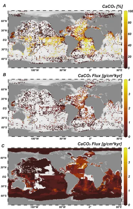
3.1. CaCO3
The database of CaCO3 content on the seafloor is the most spatially complete, with 7,792 data points
dis-tributed across all ocean basins (Figure 2a). Sediments at shallower water depths and areas with higher carbonate ion concentration in subsurface water, such as the North Atlantic, can have 80%–100% carbonate content (Archer, 1996), and near zero concentrations can be found in the deep North Pacific, the Southern Ocean and parts of the Arctic Ocean. When computed as 230Th-normalized fluxes (Figures 2b and 2c), the
North Atlantic still stands out as the highest flux region (>2 g/cm2kyr), whereas the high carbonate
con-tent regions of the Pacific have a more subdued signal due to the lower fluxes in that basin (<1 g/cm2kyr).
Interestingly, the Arabian Sea has CaCO3 fluxes nearly as high as the North Atlantic, and there is a sharp
transition from higher to lower CaCO3 fluxes in the Southern Ocean near ∼55°S in the Pacific and ∼40°S in
the Atlantic and Indian oceans. It is known that Indo-Pacific water has become more corrosive to carbonate over the course of the Holocene, on the basis of carbonate ion reconstructions and other methods (Berelson et al., 1997; Yu et al., 2010, 2014); thus, the values shown in Figure 2, which average over the entire Holo-cene, may overestimate modern conditions.
3.2. Biogenic Opal
Spatial coverage in the data available for seafloor content of biogenic opal (2,948 points) is the sparsest of the major component data. Coverage is highest in the Pacific sector of the Southern Ocean, the equatorial and North Pacific Ocean, the South Atlantic Ocean, and the Arabian Sea (Figure 3a). Relatively few data are available in the subtropical South Pacific, the subtropical North Atlantic, and the Arctic Oceans. The Antarctic Polar Front (∼60°S in the Pacific and ∼55°S in the Atlantic and Indian Ocean basins) is charac-terized by the highest opal content at about 80%. The Sea of Okhotsk and the Bering Sea also demonstrate opal contents as high as 80%. Other regions of elevated opal content are the subarctic Pacific, equatorial Pacific, equatorial Atlantic, and equatorial Indian Ocean basins, but maxima in opal there tend to be no higher than 40%.
This distribution reflects both production and preservation. Greater production of opal occurs in regions where diatoms thrive (e.g., in areas of high nutrient supply due to upwelling and/or deep winter mixing). Greater preservation in sediments, however, occurs in areas with high bulk sedimentation rates that min-imizes exposure opal to undersaturated conditions, and, especially in coastal settings, some incorporation of Al into opal which lowers its solubility (Ragueneau et al., 2000; Sayles et al., 2001; Tréguer & De La Ro-cha, 2013). For the most part, the same areas of elevated opal content stand out as areas of greater Th-nor-malized opal flux (Figure 3b), although the equatorial Pacific fluxes are somewhat more subdued due to the relatively low total fluxes there. The equatorial Pacific region provides a good example of how conclusions based on concentration alone will bias comparisons between sites or regions. Chase et al. (2015) found that in the Southern Ocean, opal flux rates were largely determined by Southern Ocean frontal dynamics
including the annual number of ice-free days. This new compilation may be useful in determining the con-trols on biogenic opal flux in other regions.
3.3. Total Organic Carbon
The distribution of available surface sediment TOC content (Figure 4a) is similar to that of biogenic opal, with much more data for the subpolar and polar North Atlantic and a fairly high density of data on many of the continental shelves. While there are more data available for TOC (6,425 points) than opal, the high con-centration of TOC data on the shelves is at the expense of deep ocean data, particularly in the South Pacific.
Figure 2. (a) Weight percentage of CaCO3, (b) flux of CaCO3 in surface sediments using spatially-interpolated
Th-normalized fluxes with discrete CaCO3% observations, and (c) flux of CaCO3 using spatially-interpolated Th-normalized
fluxes and spatially-interpolated CaCO3% values. Uncolored (white/gray) zones are shallower than 1 km or zones that
The global mean TOC content is 1.1%, and the median is 0.63%, indicating the influence of relatively high (>2%) TOC contents found on the continental shelves in the average. With regard to the continental shelves, it is important to note that a significant portion of this organic matter, in particular for deltaic sediments, is terrigenous in origin, as inferred by δ13C information (Burdige, 2005). Recently employed machine-learning
techniques also may be useful in predicting TOC contents in unobserved areas (Lee et al., 2019; Restreppo et al., 2020).
High TOC flux areas (Figures 4b and 4c) stand out near many of the eastern margins of basins, the Ber-ing Sea, the eastern Equatorial Pacific and the Arabian Sea. Due to the strong effects of preservation on TOC in sediments (Schoepfer et al., 2014), the flux patterns here are likely decoupled from surface ocean
Figure 3. (a) Weight percentage of opal, (b) flux of opal in surface sediments using spatially-interpolated Th-normalized fluxes with discrete opal % observations, and (c) flux of opal using spatially-interpolated Th-Th-normalized fluxes and spatially-interpolated opal % values. Uncolored (white/gray) zones are shallower than 1 km or zones that do not contain any Th-normalized flux observations.
productivity patterns. However, these fluxes are useful in constraining global carbon budgets as we will pursue in the discussion.
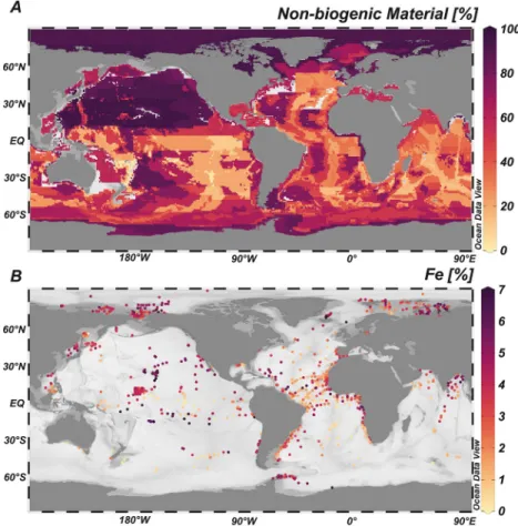
3.4. Nonbiogenic Material and Iron
We estimated the weight percentage of nonbiogenic material (Figure 5a) by using the zone averaged per-centages of CaCO3, opal, and organic matter (calculated as 1.88 g organic matter/g TOC; Lam et al., 2011)
and assuming nonbiogenic material was the remainder of the total weight. Nonbiogenic material here likely represents predominantly lithogenic material, such as aluminosilicates, except in areas with significant
Figure 4. (a) Weight percentage of TOC, (b) flux of TOC in surface sediments extrapolated using discrete TOC % observations, and (c) flux of TOC using spatially-interpolated Th-normalized fluxes and spatially interpolated TOC observations. Uncolored (white/gray) zones are shallower than 1 km or zones that do not contain any Th-normalized flux observations. TOC, total organic carbon.
authigenic metal accumulation, such as reducing sediments of the coastal ocean, or areas receiving hy-drothermal input. Less nonbiogenic material (∼10%–20%) is found on the mid-ocean ridges because of the higher percentage of CaCO3 preserved there. In all the deep basins, the nonbiogenic percentage increases
with depth and approaches 90%–100% in the deep North Pacific and Arctic basins, in part because of the lack of other particle phases preserved there.
We present these data together with the Fe weight percentage compilation, containing 1,210 points (Fig-ure 5b), since Fe in the ocean is predominantly associated with lithogenic and authigenic sediments. Fe and our estimate of nonbiogenic material have similar distributions overall, with higher Fe content in all deep basins as well as in the Arctic Ocean and most marginal seas. Fe is on average 3.9% in the upper continental crust (Rudnick & Gao, 2014), but this Fe fraction will of course vary depending on the source of the litho-genic material. The average lower continental crust is 6.7% Fe (Rudnick & Gao, 2014); the average oceanic crust (mid-ocean ridge basalt) is 8.1% Fe (White & Klein, 2013); and metalliferous sediments underlying sites of hydrothermal vents can be considerably more enriched (Boström et al., 1969). The Fe concentra-tions of samples included in this ocean sediment database range from 0.02% to ∼20% Fe, with a median of 3.1%. The distribution of the Fe/Al ratio (Figure 6; note not all Fe data points had available Al data) is one indication of the source of iron, as the upper continental crust has a Fe/Al weight ratio of 0.48 (Rudnick & Gao, 2014) and mid-ocean ridge basalts have a ratio of 1.01 (White & Klein, 2013). Excluding highly Fe enriched samples with Fe/Al > 1.5, about 50% of the ratio observations are near or below the upper conti-nental crust average. Areas with enriched Fe/Al ratios include GEOTRACES expedition GP16 (∼10°–20°S, 90°–140°W), which underlies an extended hydrothermal plume emanating westward from the East Pacific Rise (Fitzsimmons et al., 2017; Resing et al., 2015).
Figure 5. The weight fractions of nonbiogenic material (a) and Fe (b) in the global ocean. The Fe estimates are from discrete cores in the database and the nonbiogenic material is based on the 1° resolution interpolated major component fractions, assuming nonbiogenic material is the residual between 100% and the percentages of CaCO3, opal, and organic
Additional enriched areas include other sites from Southern East Pacific Rise, the Mid-Atlantic and Central Indian Ridges, sites near basaltic oceanic islands, including Hawaii and Iceland, as well as several continen-tal margin areas including the Sea of Cortez, the northern Gulf of Mexico, and the shallow Arctic seas. This demonstrates that both hydrothermal input and coastal authigenic metal formation have imprints on the global Fe distribution in addition to lithogenic material such as dust.
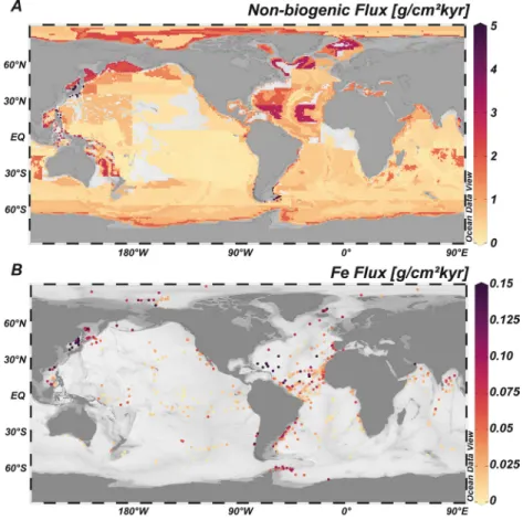
When converted to flux, the overall similarity of nonbiogenic material and Fe flux is again apparent (Fig-ure 7). Despite higher concentrations in the North Pacific basin, the nonbiogenic material and Fe fluxes are lower in the North Pacific Ocean than in the deep North Atlantic Ocean. The higher fluxes in the Atlantic basin are likely indicative of the large lithogenic flux of Saharan dust to the North Atlantic Ocean in addi-tion to other coastal sources, such as rivers or margin sediments. Many of the marginal seas have elevated Fe and nonbiogenic material fluxes reflecting coastal sources.
3.5. Mercury
Spatial coverage for surface sediment Hg concentrations is the most sparse of the components considered here (320 observations; Figure 8a). Observations in the Northern Hemisphere and on continental margins are much more prevalent than in the Southern Hemisphere or in the central basins. In the Atlantic Ocean, high continental runoff may cause higher sediment Hg levels on its continental shelves (58 ± 97 ppb) com-pared to its deep basin sediments (38 ± 21 ppb). In the Pacific Ocean, there are higher Hg concentrations in the Humboldt Upwelling System (202 ± 85 ppb) compared with the deep Pacific Ocean (71 ± 46 ppb), and this may be due to higher particulate Hg export in the productive upwelling region. Smaller basins, such as the Black Sea and the Mediterranean Sea are characterized by relatively high sediment Hg concentrations (149 ± 47 ppb and 86 ± 76 ppb, respectively). As more data on Hg concentrations in seawater become avail-able (e.g., Bowman et al., 2015, 2016; Cossa et al., 2009, 2018; Kim et al., 2017; Rosati et al., 2018), we may be able to further link some of these basin sedimentary differences to water column processes.
While the conversion to Hg flux also results in sparse estimates, both with discrete Hg observations (Fig-ure 8b) or zone-averaged Hg observations (Figure 8c), we consider how the Hg fluxes derived here compare with other global or basin-wide estimates which remain highly uncertain. Note in Figure 8c that the South Pacific Subtropical Gyre is a single Longhurst province (Figure 1) between the margins of Australia and South America. With observations only on the western edge of this province, the interpolation scheme extends the flux estimate to much of the South Pacific. When integrated across zones, our estimate provides nearly full coverage of the Arctic Ocean deeper than 1,000 m (Figure 8c and Figure S11). The integrated Arctic Hg flux is 4.4 ± 0.7 Mg/yr, which is consistent with a recent estimate in the deep Arctic (4 ± 3 Mg/ yr) that derived fluxes by assuming a constant sedimentation rate (Tesán Onrubia et al., 2020). The un-certainty in our flux estimate is a minimum as it only accounts for unun-certainty in the Th-normalized flux
Figure 6. Fe/Al weight ratio in the global sediment composition database. The upper continental crust has an average ratio of 0.48 g/g and mid-ocean ridge basalts have a ratio of 1.01 g.g. Note in comparison to Figure 5, only a subset of Fe datapoints had available Al data.
interpolation. There are too few Hg data presently available to statistically assess the uncertainty in Hg interpolation. While coverage across the interpolation zones globally is not complete, we can nonetheless attempt a global integration. To do this, we assumed the average fluxes in the North Pacific apply to the en-tire North Pacific, the average fluxes in the South Pacific apply to the enen-tire South Pacific and Indian Ocean, and the average fluxes in the North Atlantic apply to the entire Atlantic basin (using surface areas defined by ETOPO1). This produces a global deep-sea burial rate of 220 ± 40 Mg Hg/yr. Because the Th-normalized flux observations are confined to the deep ocean (>1000 m), our integration misses a likely considerable flux on the continental shelves and upper continental slopes. Our estimate of deep-sea Hg burial is close to another recent study, 360 Mg/yr (Zhang et al., 2015), and significantly smaller than the 600 Mg/yr (Outridge et al., 2018) and 1540 Mg/yr (Amos et al., 2014) made in other studies. It will require more observations of deep-sea and continental margin Hg concentrations to resolve this issue.
3.6. Excess Barium
Our database contains 1,457 estimates of Baxs. As a relatively minor component of the sediments (0–∼5000
ppm), Baxs weight fractions are influenced by dilution of the varying total sediment flux, for instance with
lower weight fractions in the North Atlantic versus the North Pacific on average (Figure 9a). When converted to flux (Figure 9b), there are higher Baxs fluxes in the eastern equatorial Pacific, the subarctic Pacific, across
several frontal zones in the Southern Ocean, and in the Arabian Sea, with lower fluxes found in the central Pacific, the tropical Atlantic and the Arctic. Importantly, barite, the main carrier of Baxs, is not preserved in
sulphate reducing sediments (Riedinger et al., 2006; Torres et al., 1996); hence, areas like upwelling zones or restricted basins may not preserve the original deposition flux. There may also be preservation effects on Baxs accumulation under oxic or suboxic conditions, including bottom waters undersaturated with respect
to barite, which have not yet been thoroughly determined (McManus et al., 1998; Paytan & Griffith, 2007;
Figure 7. Th-normalized flux of (a) nonbiogenic material based on spatially interpolated mass flux and CaCO3, opal
Serno et al., 2014; Van Beek et al., 2003). We examine the relationship between our derived Baxs fluxes and
indicators of biological productivity in the discussion.
The spatial coverage of Baxs flux observations is sufficient to estimate the global deep-sea burial (Figure 9c)
as 2.6 ± 1.4 Tg Ba xs/yr. This is very close, though with a significant uncertainty, to a previous estimate of 2.5 Tg/yr (Dickens et al., 2003; Paytan & Kastner, 1996). This prior estimate assumed a steady-state between Ba burial and the supply of dissolved Ba by rivers (estimated as 2.2 Tg/yr) and hydrothermal vents (estimat-ed as 0.5 Tg/yr). Paytan and Kastner (1996) based these fluxes on data available at the time from the Congo, Amazon and Mississippi Rivers (Edmond et al., 1978) and hydrothermal vent observations from the East
Figure 8. (a) Hg concentrations, (b) flux of Hg in surface sediments extrapolated using discrete Hg observations, and (c) flux of Hg using spatially-interpolated Th-normalized flux and zone-averaged Hg observations. Note in many cases here a limited number of observations are interpolated across relatively large interpolation zones, for example, in the South Pacific Subtropical Gyre and around Antarctica.
Pacific Rise (Von Damm et al., 1985). The magnitude of Ba sources is currently being assessed (e.g., Horner et al., 2020), including evidence for other sources such as submarine groundwater discharge or cold seeps. Because of the uncertainty in our Ba burial estimate, it is premature to conclude whether or not there is a steady-state balance between burial and known sources.
4. Discussion
4.1. Deep-Sea Burial of CaCO3, Opal, and TOC
Using the spatially interpolated flux maps of CaCO3, opal and TOC, we can integrate across the global
ocean and estimate a burial flux of these components to the deep sea (>1 km depth) based entirely on
Figure 9. (a) Baxs concentration, (b) Baxs fluxes based on spatially-interpolated Th-normalized fluxes and discrete
Baxs observations and (c) Baxs flux based on spatially-interpolated Th-normalized fluxes and zone-averaged Baxs
Th-normalized fluxes. These fluxes of C and Si are critical to understand-ing their global cyclunderstand-ing and turnover rates. Our Th-normalized flux inter-polation only extends to the 87% of the seafloor for which data are avail-able and thus our summed burial rates will underestimate global burial. 4.1.1. CaCO3 Burial
The deep-sea burial of CaCO3 derived from our interpolation is
136 ± 34 Tg C/yr. Cartapanis et al. (2018) discuss that the range of exist-ing deep-sea CaCO3 burial estimates is 100–150 Tg C/yr, strikingly in-line
with our estimate (Figure 10). To examine our estimate further, we look at the relative contributions of the ocean basins to the total CaCO3 burial.
In our flux estimations, the following fractions of CaCO3 flux were buried
in the Atlantic (40%), Pacific (22%), Indian (20%), Southern (17%), and Arctic (0.4%) Oceans. The basin boundaries were defined using the Long-hurst provinces in Figure 1. These percentages compare well to the rang-es for the basin CaCO3 flux percentages from Cartapanis et al. (2018),
based on a smaller data set of Th-normalized fluxes, and from the mod-el of Dunne et al. (2012): Atlantic (41%–48%), Pacific (25%–27%), Indi-an (24%–34%), Antarctic (0%), Indi-and Arctic (1%). The main difference in this comparison is that Cartapanis et al. (2018) calculated the Antarctic Ocean as only south of 60°S, whereas in our calculation the Longhurst provinces consider the Southern Ocean south of roughly 40°S. The continental shelves and shallow water environments are expected to have a CaCO3 burial rate of around 150 Tg C/kyr for a total of ∼300 TgC/yr
(Milliman, 1993). Thus, our estimates of CaCO3 burial appear to be consistent with previous work.
4.1.2. Biogenic Opal Burial
The deep-sea burial of opal derived here, given in terms of Si, is 153 ± 33 Tg Si/yr. Of this total, the South-ern Ocean (>40°S) deep-sea Si burial is 75 ± 17 Tg Si/yr. This is consistent, within uncertainties, with that derived by Chase et al. (2015) for the deep Southern Ocean of 64 ± 28 Tg Si/yr. This is as to be expected as Chase et al. (2015) used a very similar approach as the present study, involving Th-normalized opal flux observations interpolated across biological provinces. Outside of the Southern Ocean then, our study esti-mates a biogenic opal burial of 78 ± 17 Tg Si/yr in the deep sea north of 40°S. Because of the finding that XRD methods for opal determination were significantly higher than other methods (Conley et al., 1998), as a sensitivty analysis we re-ran the interpolation process, excluding data points produced by the XRD method. This did not significantly alter the results within our uncertainty (the resulting fluxes excluding XRD data were total deep-sea burial of 152 ± 33 Tg Si/yr, Southern Ocean burial of 71 ± 16 Tg Si/yr and non-Southern Ocean burial of 81 ± 18 Tg Si/yr). Our estimated deep-sea burial of 153 Tg Si/yr is a signif-icant upward revision from previous estimates of 98 Tg Si/yr (DeMaster, 2019) and 70 Tg Si/yr (Tréguer & De La Rocha, 2013). We have determined that most of the upward revision is due to increased burial rates in the non-Antarctic deep sea.
The latest prior estimates in the literature for deep-sea biogenic Si burial outside of the Southern Ocean mainly derive from the work of DeMaster (1981), who calculated a non-Antarctic deep-sea burial of 29 Tg Si/yr. This value has been used without significant modification in most subsequent assessments of the glob-al silica cycle (DeMaster, 2002; Ragueneau et al., 2000; Tréguer & De La Rocha, 2013; Tréguer et al., 1995). DeMaster (2019) used a slightly higher non-Antarctic deep-sea burial of 34 Tg Si/yr. Still, this estimate is more than a factor of 2 lower than our estimate of 78 Tg Si/yr. DeMaster (1981) estimated this burial flux based on basin-averaged biogenic silica content and bulk mass accumulation rates for basins assumed to be responsible for the majority of deep-sea silica burial, namely the Bering Sea (14 Tg/yr), the North Pacific (8.4 Tg/yr), the Sea of Okhotsk (5.6 Tg/yr), and the Equatorial Pacific (0.6 Tg/yr). A maximum burial esti-mate for the rest of the deep sea, assumed to be very low in silica content, was also included (<0.2 Tg/yr). The Si burial rates from our interpolation (using only water depths >1000 m) for these basins are: Bering Sea (2.6 Tg/yr), North Pacific (4.4 Tg/yr, within the geographic box used by DeMaster, 1981, bound by the northern margin and 35°N from Asia to 170°E and the box bound by the northern margin and 42°N be-tween 170°E and North America), Sea of Okhotsk (2.2 Tg/yr), and the equatorial Pacific (5.6 Tg/yr, using
Figure 10. Comparison of globally integrated deep-sea (>1,000 m) fluxes of CaCO3, opal, and TOC from this and other studies (Burdige, 2007;
Cartapanis et al., 2018, 2016; DeMaster, 2019; TDLR2013 = Tréguer & De La Rocha, 2013).
the box bound by 3°N, 6°S, 170°W, and 79°W, representing a similar area to that considered by DeMas-ter, 1981). The remainder of the deep sea north of 40°S contains burial of 61 Tg Si/yr. Thus, our estimates revise downward (by factors less than 10) the estimates from the Bering Sea, the North Pacific and the Sea of Okhotsk, possibly due to the impact of sediment focusing on the mass accumulation rates assumed by DeMaster (1981) for these regions. At the same time, our estimates are significantly higher in Si burial in the Equatorial Pacific and the remaining ocean. Not available to DeMaster (1981) at the time, our new compila-tion of opal concentracompila-tion data (2,399 deep-sea points) shows there are in fact many regions outside of the assumed “hot spots” for opal burial that contain opal in excess of 10%, such as the northeast Atlantic and equatorial Indian (Figure 3). Additionally, Th-normalized burial rates constrained for nearly all (87%) of the deep sea can properly account for the magnitude of opal burial even in sediment of low opal concentration. By basin, our calculated deep-sea opal burial was found in the following: 11% (Atlantic), 24% (Pacific), 15% (Indian), 49% (Southern), and 0.2% (Arctic).
Recent estimates of biogenic silicon burial on the continental margins range from 235 ± 118 Tg Si/yr (Rah-man et al., 2017; Treguer et al., 2021) to 140 ± 30 Tg Si/yr (DeMaster, 2019). The burial of silicon associated with siliceous sponges, also mainly found on continental margins, may be another significant flux (48 Tg Si/yr according to Maldonado et al., 2019 or 25 Tg Si/yr at most, according to DeMaster, 2019). Thus, our estimate of deep-sea biogenic Si burial of 153 Tg/yr could be on par to the continental margin sink in global ocean Si burial. In other words, roughly 50% of the burial sink of Si in the ocean occurs in the deep sea. 4.1.3. TOC Burial
Our deep-sea TOC burial rate is 20 ± 6 Tg C/yr. This is similar to the estimate of Cartapanis et al. (2016) of 17 Tg C/yr that used Th-normalized fluxes where possible. In contrast, another available estimate of deep-sea (>1000 m) organic carbon burial is higher, 86 Tg C/yr (Burdige, 2007), based on organic carbon remin-eralization rates (Figure 10). Another study (Dunne et al., 2007) estimated TOC burial of 12 TgC/yr in wa-ters deeper than 2000 m based on available composition data and bulk accumulation rates (Jahnke, 1996). The equivalent flux (below 2 km) in our assessment is 17 ± 5 TgC/yr, which is in line with the Dunne et al. (2007) estimate. The fractional contributions to TOC burial for the different basins in our estimate are: Atlantic (28%), Pacific (39%), Indian (15%), Southern (15%), and Arctic (3%). This is fairly similar to the frac-tional contribution to surface area in the deep sea using the Longhurst definitions: Atlantic (21%), Pacific (41%), Indian (13%), Southern (22%), and Arctic (4%), perhaps indicating a slightly outsized contribution from the Atlantic and reduced contribution from the Southern Ocean to the global deep-sea TOC burial on a per area basis. Many studies recognize that a large proportion of organic carbon is buried in the continental margin environment, such as Burdige’s (2007) estimate of a 222 TgC/yr in water shallower than 1000 m, giving a total ocean burial rate of 309 TgC/yr (Figure 10). In summary, the deep-sea fluxes derived here will help constrain budgets of C and Si, though the significant coastal ocean fluxes likely cannot be constrained by Th-normalization and should be pursued by other methods.
4.2. Imprints of Biological Productivity in Sedimentary Fluxes
As these have all been used for paleo-proxies of biological productivity in the ocean, we compared our sedimentary fluxes of opal, TOC and Baxs to estimates of net primary productivity (NPP) and export
pro-ductivity (EP) in the modern ocean (maps of the NPP and EP used shown in Figure S15). For net primary productivity, we used the satellite-based Carbon, Absorption, and Fluorescence Euphotic-resolved (CAFE) algorithm (Silsbe et al., 2016), using monthly data from the Oregon State University Ocean Productivity webpage (http://sites.science.oregonstate.edu/ocean.productivity/) averaged over 1 decade (2003–2012), which provided estimates at 1/6°-resolution. For export productivity, we used a satellite- and ocean tracer observation-constrained estimate of the flux of particulate organic carbon out of the euphotic zone (DeVries & Weber, 2017), available at 2°-resolution. Each flux data point (i.e., as plotted in Figures 3b, 4b, and 9b) in our database was matched with the closest grid point in the NPP and EP estimates. We also compared discrete observations for which Th-normalized flux (at >1000 m water depth) and component composition were measured on the same core (n = 444 for opal flux, n = 247 for TOC flux, and n = 211 for Baxs flux) to
NPP and EP, to remove the uncertainty associated with spatial interpolation. It is only for the relationships with these directly observed component fluxes that we report correlation statistics below.
Despite their association with biological productivity, opal flux, TOC flux, and Baxs flux all have weak linear
correlations with NPP and EP (Figure 11; all r values < 0.5). For opal, there is an apparent negative rela-tionship (which is statistically significant at 95% confidence for opal flux vs. NPP) that can be seen with the highest opal fluxes mostly on the lower end of the spectra of NPP (10–15 g C/cm2kyr) and EP (2–3 g
C/cm2kyr). This is largely due to areas of the Southern Ocean which are relatively low in NPP and EP on
the annual average but are among the most productive regions for diatoms and opal particle flux (Honjo et al., 2008) (Figure 3). In TOC, there are weak but significant positive linear correlations between TOC flux and NPP and EP, although a large number of points with very low TOC flux (<0.05 gC/cm2kyr) exhibit a
Figure 11. (a–f, respectively) Comparisons and linear correlation analyses between deep-sea opal flux, total organic carbon (TOC) flux, and Baxs flux derived from the present study with net primary productivity (a, c, e) and export
productivity estimates (b, d, f) (DeVries & Weber, 2017; Silsbe et al., 2016). Colored points are based on spatially-interpolated fluxes and black points are direct component and Th-normalized flux observations for the same core. The insets display the linear regression slope (m, with e indicating power of 10 exponent) and Pearson correlation coefficient (r, bold indicating statistical significance at 95% confidence).
large range in NPP (10–35 g C/cm2kyr) and EP (0–10 g C/cm2kyr). Schoepfer et al. (2014) found that if
pres-ervation effects on organic carbon could be accounted for using variations in bulk sediment accumulation rates, there were significant relationships between a smaller compilation of TOC Holocene burial and NPP and EP estimates; however, that study relied only on bulk organic carbon accumulation rates and, thus, may have been biased by sediment focusing and/or age model errors in the data included. Furthermore, other synthesis work (LaRowe et al., 2020) suggests that organic carbon preservation is complex and depends on many ecological factors in addition to oxygen levels and bulk sedimentation rate.
With regard to Baxs, we found a weak but significant positive linear correlation with EP and no significant
relationship with NPP. Schoepfer et al. (2014) also found no significant relationships between a smaller data compilation of bulk Baxs accumulation rates and estimates of NPP and EP. Dymond et al. (1992) noted
that some preservation effects were apparent in early comparisons between Baxs in the sediments of
differ-ent basins and these authors proposed a correction-scheme for Ba preservation effects based on the bulk accumulation rate and the dissolved Ba content in deep waters which varies from basin to basin. Schoepfer et al. (2014) attempted those corrections and still did not find a signficant relationship with productivity pat-terns. In the present study, we do not have bulk accumulation rates in the data set and thus cannot attempt the Dymond et al. correction; however, we do show that Th-normalized Ba fluxes, which should get as close as possible to the seafloor rain of Baxs, still do not show a strong relationship with productivity patterns
globally. Eagle et al. (2003) did find that relationships between sediment Baxs and productivity indicators
appeared to vary between basins. It is beyond the scope of this study to investigate the possible regional relationships in Baxs flux but this could be done in future work.
The general conclusion we can draw from this comparison is that productivity indicators such as the flux of opal, TOC and Baxs are not simply related to the spatial pattern of productivity in the global ocean and
likely several preservational effects must modulate their burial fluxes in ways that need further investiga-tion. In the case of opal, there is a known divergence in production patterns, as diatoms, the main produc-ers of biogenic opal, have a distinct biogeography compared to net primary production (e.g., Kostadinov et al., 2010, 2016). Baxs may have preservation effects that are yet to be fully understood, likely involving
the effects of water column undersaturation, bulk mass accumulation rates and the redox state of the sedi-ments. Furthermore, the uncertainties associated with the lithogenic correction on bulk Ba concentrations may obscure relationships with biogenic barite. These results do not preclude, however, the use of these proxies at individual sites or perhaps regional studies in which the change in the proxy with time is inter-preted as a change in productivity. The present analysis is focused on global deep-sea spatial patterns as opposed to temporal patterns. Furthermore, average fluxes over the Holocene could considerably differ from satellite-derived productivity estimates which are based mainly on data from the past 20 years. Lastly, the NPP and EP products we have chosen, although state-of-the-art, still contain uncertainty themselves, for example, in matching field measurements (DeVries & Weber, 2017; Silsbe et al., 2016). Thus, there are limits to our ability to evaluate the extent to which biological productivity patterns are embedded within the distribution of the proxy burial rates.
4.3. Imprints of Deep Particulate Flux in Sedimentary Fluxes
While it proved challenging to find the imprint of near surface productivity in our sedimentary database, we explored the relationship of our burial fluxes to subsurface particle fluxes. Deep particle fluxes have under-gone some regeneration/dissolution processes since being exported from the surface but have not yet expe-rienced diagenesis at the seafloor while being buried. The knowledge of deep particulate flux is much more limited than either surface or bottom fluxes, but this information is critical especially for the interpretation of paleo-productivity proxies. The information we have is mainly limited to sediment trap studies, although the GEOTRACES program is currently mapping out deep particulate fluxes on transect cruise studies using in-situ pumped particulate 230Th (Hayes et al., 2018; Pavia et al., 2019).
For our comparison here, we use the deep sediment trap compilation of Honjo et al. (2008), that compiled available sediment trap data from 135 sites for CaCO3, opal and TOC and normalized all the data to a
com-mon depth of 2 km, or the mesopelagic-bathypelagic boundary (Figure S13). The sedimentary CaCO3 fluxes