Distribution of epipelagic metazooplankton across the Mediterranean Sea during the summer BOUM cruise

(1)

HAL Id: hal-02008131

https://hal.archives-ouvertes.fr/hal-02008131

Submitted on 3 Aug 2020

HAL is a multi-disciplinary open access

archive for the deposit and dissemination of

sci-entific research documents, whether they are

pub-lished or not. The documents may come from

teaching and research institutions in France or

abroad, or from public or private research centers.

L’archive ouverte pluridisciplinaire HAL, est

destinée au dépôt et à la diffusion de documents

scientifiques de niveau recherche, publiés ou non,

émanant des établissements d’enseignement et de

recherche français ou étrangers, des laboratoires

publics ou privés.

Distribution of epipelagic metazooplankton across the

Mediterranean Sea during the summer BOUM cruise

A. Nowaczyk, F Carlotti, D. Thibault-Botha, M. Pagano

To cite this version:

A. Nowaczyk, F Carlotti, D. Thibault-Botha, M. Pagano. Distribution of epipelagic metazooplankton

across the Mediterranean Sea during the summer BOUM cruise. Biogeosciences, European Geosciences

Union, 2011, 8 (8), pp.2159-2177. �10.5194/bg-8-2159-2011�. �hal-02008131�

(2)

www.biogeosciences.net/8/2159/2011/ doi:10.5194/bg-8-2159-2011

Biogeosciences

Distribution of epipelagic metazooplankton across the

Mediterranean Sea during the summer BOUM cruise

A. Nowaczyk, F. Carlotti, D. Thibault-Botha, and M. Pagano

Aix-Marseille Université, UMR6535, INSU-CNRS – Laboratoire d’Océanographie Physique et Biogéochimique, Centre d’Océanologie de Marseille, Campus de Luminy, Case 901, 13288 Marseille, France

Received: 14 March 2011 – Published in Biogeosciences Discuss.: 22 March 2011 Revised: 29 July 2011 – Accepted: 1 August 2011 – Published: 9 August 2011

Abstract. The diversity and distribution of epipelagic meta-zooplankton across the Mediterranean Sea was studied along a 3000 km long transect from the eastern to the western basins during the BOUM cruise in summer 2008. Metazoo-plankton were sampled using both a 120 µm mesh size bongo net and Niskin bottles in the upper 200 m layer at 17 stations. Here we report on the stock, the composition and the struc-ture of the metazooplankton community. The abundance was 4 to 8 times higher than in several previously published stud-ies, whereas the biomass remained within the same order of magnitude. An eastward decrease in abundance was ev-ident, although biomass was variable. Spatial (horizontal and vertical) distribution of metazooplankton abundance and biomass was strongly correlated to chlorophyll-a concentra-tion. In addition, a clear association was observed between the vertical distribution of nauplii and small copepods and the depth of the deep chlorophyll maximum. The distinction between the communities of the eastern and western basins was clearly explained by the environmental factors. The spe-cific distribution pattern of remarkable species was also de-scribed.

1 Introduction

Although the Mediterranean Sea represents only ∼0.82 % of the total surface of the global ocean, it is the largest quasi-enclosed sea composed of two large basins, the eastern and the western basins, separated by the Strait of Sicily, which are subsequently divided in several sub-basins. It could be assimilated to a mini-size ocean with continental shelves, deep basins and trenches. The surface circulation is driven mainly by the inflow of Atlantic water through the Strait

Correspondence to: A. Nowaczyk (antoine.nowaczyk@univmed.fr)

of Gibraltar, its signature being modified as it travels east-ward. The Mediterranean is displaying deep water mass for-mation sites which have shown large modifications through time (Pinardi and Masetti, 2000; Millot and Taupier-Letage, 2005; and review by Bergamasco and Malanotte-Rizzoli, 2010). It is a hot spot for marine biodiversity (Margalef, 1985; Bianchi and Morri, 2000; Coll et al., 2010) with a marine biota composed of endemic and allochtonous species of Atlantic and Red Sea origins (Furnestin, 1968; Bianchi and Morri, 2000). This ecosystem is overall oligotrophic, but paradoxically, significant production do occur which sustain large fisheries and marine mammals communities (Coll et al., 2010; W¨urtz, 2010). This “maxi-size laboratory” can be then considered as one of the most complex marine environment (Meybeck et al., 2007).

As a whole, the Mediterranean Sea is characterized by a strong eastward gradient in nutrients, phytoplankton biomass and primary production (reviewed in Siokou-Frangou et al., 2010) with ultra-oligotrophic conditions being found in the Levantine basin (Krom et al., 1991; Ignatiades, 2005; Moutin and Raimbault, 2002). From a handful of studies, a similar pattern has also been reported at the basin scale for meso-zooplankton abundance (Dolan et al., 2002; Siokou-Frangou, 2004; Mazzocchi et al., 1997; Minutoli and Guglielmo, 2009) but no synoptic view through the western and east-ern basins was run to confirm this trend. Moreover, no clear pattern was highlighted for the biomass which presents sev-eral hot spots located in the north-western Mediterranean, the Catalan Sea, the Algerian Sea and the Aegean Sea (re-viewed in Siokou-Frangou et al., 2010). Currently, the ex-isting datasets are not yet sufficient to get a comprehen-sive understanding of the metazooplankton distribution in the Mediterranean Sea.

Indeed, many field studies have been realised at regional scales and have highlighted the impact of mesoscale features on the distribution and diversity of metazooplankton in both Mediterranean basins (Ibanez and Bouchez, 1987; Pinca and

(3)

2160 A. Nowaczyk et al.: Distribution of epipelagic metazooplankton Dallot, 1995; Youssara and Gaudy, 2001; Mazzocchi et al.,

2003; Siokou-Frangou, 2004; Pasternak et al., 2005; Riandey et al., 2005; Fernandez de Puelles et al., 2004, 2007; Zer-voudaki et al., 2006; Molinero et al., 2008; Licandro and Icardi, 2009; Siokou-Frangou et al., 2009). Mesoscale hy-drodynamic structures are known also to enhance nutrient concentrations, and therefore, plankton patchiness stimulat-ing trophic transfers towards large predators.

The BOUM experiment (Biogeochemistry from the Olig-otrophic to the Ultra-oligOlig-otrophic Mediterranean) was con-ducted in order to obtain a better representation of the inter-actions between planktonic organisms and the cycle of bio-genic elements in the Mediterranean Sea across the western and eastern basins through a 3000 km survey. Our main goal here was to improve our knowledge on the role of plank-tonic metazoan (metazooplankton hereafter; Sieburth et al 1978) in the biogeochemical cycle in such an open olig-otrophic ecosystem by coupling standing stock estimations (abundance, biomass, and size classes) and metabolic mea-surements. The presentation of this work is carried out in two steps. The structural investigation is presented here and the functional part will be presented in another manuscript (Nowaczyk et al., 2011). Therefore, the present study inves-tigates the metazooplankton community spatial distribution (vertical and horizontal) including small-size copepods (nau-plii and different copepodite stages) often neglected in previ-ous studies. Finally, we attempt to define the links between the spatial distribution of metazooplankton and the environ-mental characteristics.

2 Materials and methods

2.1 Cruise track and environmental parameters 2.1.1 Cruise transect

A 3000 km transect across the Mediterranean Sea was conducted during the BOUM cruise from 18 June to 20 July 2008 on board the French N.O. L’Atalante (Fig. 1). The cruise run eastward from the Ionian basin (IB) to the Levantine basin (LB) from 18 June to 29 June; then switched

to a westward direction. After a transit period of three

days, sampling continued from the Ionian basin through the Sicily Channel (SC), the Algero-Provencal basin (APB) to the Rhˆone River Plume (RRP). Sampling strategy consisted in 27 short-stay stations (∼2–3 h) distributed ∼100 km apart and long-stay stations (4 days: stations A, B and C) located in the centre of important hydrological features (anticyclonic gyres) (see Moutin et al., 2011 for more details). Loca-tion of the sampling staLoca-tions is presented in Fig. 1 and Ta-ble 1. Physico-chemical parameters and phytoplankton were sampled at all stations whereas the metazooplankton, ciliates and heterotrophic nanoflagellates (HNF) were samples every other stations.

2.1.2 Sampling and analysis of environmental parameters

Vertical profiles of temperature, conductivity and oxygen were obtained using a Sea-Bird Electronic 911 PLUS CTD. Nutrients, chlorophyll, ciliates and HNF were sampled us-ing Niskin bottles. Ammonium and phosphate concentration were immediately measured on board with an auto-analyzer (Bran+Luebbe auto-analyseur II) according to the colorimet-ric method as fully described in Pujo-Pay et al. (2011). To-tal chlorophyll-a was measured by the fluorimetric meth-ods following a methanol extraction (Herbland et al., 1985). HNF samples were filtered onto black nucleopore filters and stained with DAPI (Porter and Feig, 1980) and stored

at −20◦C on board until analysis, then enumerated using

LEITZ DMRB epifluorescence microscope. Ciliates samples were fixed in 2 % Lugol’s iodine-seawater solution, stored

at 4◦C and counted using an inverted microscope. These

two methods were fully described in Christaki et al. (2011). The same method was used for nanophytoplankton and di-atoms identification. The particular organic matter was de-termined according to the wet oxydation procedure described by Raimbault et al. (1999).

2.2 Zooplankton 2.2.1 Sampling strategy

Zooplankton was collected within the upper 200 m layer (100 m at st. 17 and 27) using double Bongo nets (60 cm mouth diameter) fitted with 120 µm mesh size and equipped with filtering cod ends. Vertical hauls were done at a speed of 1 m s−1. No flowmeters were available but special care was taken while sampling to keep the cable vertical. Volume sampled by the net was then reported to the depth of the tow and the opening surface of the net (0.28 m2). Due to wire time constraints sampling was performed at different times of day and night. The length of time spent at stations A, B and C allowed us to collect zooplankton 3 times at noon and 4 times at midnight, on consecutive days.

Immediately after collection, the cod-end content of the first net was kept fresh and split into two parts with a Motoda box. The first part was processed immediately for biomass

measurements. The second half of the sample was

col-lected onto a GF/F filter, placed in a Petri dish, and then deep frozen in liquid nitrogen for further ingestion rates mea-surements (Nowaczyk et al., 2011). The cod-end content of the second net was directly preserved in 4 % buffered formalin-seawater solution for later taxonomic identification and abundance measurements. Discrete sampling was also performed to study vertical distribution of copepod nauplii and small copepods from water samples collected with the CTD/rosette. At each selected depth, the content of a 12 L Niskin bottle was gently collected onto a 20 µm mesh net and fixed in a 2 % Lugol’s iodine-seawater solution. Seven

(4)

A. Nowaczyk et al.: Distribution of epipelagic metazooplankton 2161 27 25 24 21 19 17 15 13 ₁ 3 5 ₇ ₉ 11 26 23 22 20 18 16 14 12 2 ₄ ₆ 8 ₁₀ De p th ( m ) 0 1 000 2 000 3 000 0 -1 000 -2 000 -3 000 -4 000 Distance (km) Algero-provencal basin Ionian basin Levantine basin Sicily channel A B C 27 25 24 21 19 17 15 13 1 3 5 7 9 11 Leg 1 Leg 2

Western basin Eastern basin

Fig. 1. (a) Location of sampling stations superimposed on a SeaWIFS composite image of the

sea surface integrated chlorophyll a concentration (permission to E.Bosc) during the BOUM transect (June 16th – July 20th 2008). Short-stay stations where zooplankton was sampled (white) and not sampled (black) and long-stay stations (red). (b) Bottom depth and geographic areas along the transect.

Latitu de ° N (a) (b) Longitude ° E Chlorophyll a (m g m -3 )

Fig. 1. (a) Location of sampling stations superimposed on a SeaWIFS composite image of the sea surface integrated chlorophyll-a con-centration (permission to E.Bosc) during the BOUM transect (16 June–20 July 2008). Short-stay stations where zooplankton was sampled (white) and not sampled (black) and long-stay stations (red). (b) Bottom depth and geographic areas along the transect.

depths were sampled between the surface and 200 m depth at stations A, B and C and only to a depth of 150 m at short-stay stations. The sampling depths were distributed according to the deep chlorophyll maximum depth.

2.2.2 Biomass measurement

The subsample for bulk biomass measurement was filtered onto pre-weighted and pre-combusted GF/F filter (47 mm) which was quickly rinsed with distilled water and dried in

an oven at 60◦_{C for 3 days onboard. Dry-weight (mg) of}

samples was calculated from the difference between the fi-nal weight and the weight of the filter and biomass (mg DW m−3)was extrapolated from the total volume sampled by the net. Once back on land, carbon and nitrogen contents were measured. Dried samples were grinded, homogenized then split into 3 equal fractions (∼0.8–1 mg DW), placed in tin caps and analyzed with a mass spectrometer (INTEGRA CN, SerCon).

2.2.3 Microscope counts

Taxonomic identification and counts of zooplankton were done back in the land laboratory using a LEICA MZ6 dis-secting microscope. Very common taxa were counted in sub-samples (1/32 or 1/64), and the whole sample was examined for either rare species and/or large organisms (i.e. euphausi-ids, amphipods). Identification of the copepods community was made down to species level and developmental stage when possible. Sex determination was also done on the most abundant species. Species/genus identification was made ac-cording to Rose (1933), Tr´egouboff and Rose (1957) and Ra-zouls et al. (2005–2011). Holoplankton organisms other than copepods as well as meroplankton were identified down to taxa levels.

2.2.4 Digital imaging approach using the Zooscan After homogenization, another fraction of each preserved sample containing a minimum of 1000 particles was placed

(5)

2162 A. Nowaczyk et al.: Distribution of epipelagic metazooplankton

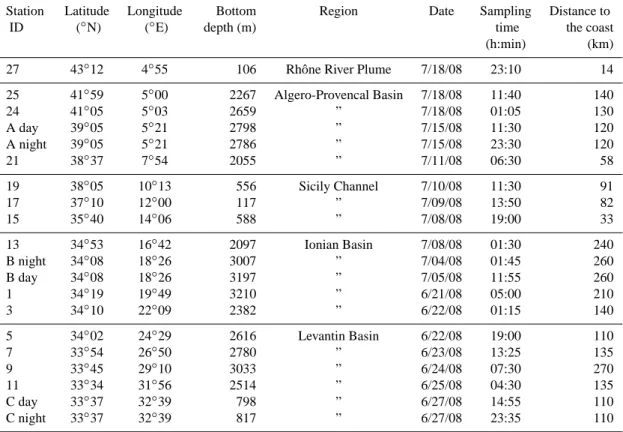
Table 1. Position and characteristics (latitude, longitude, bottom depth, geographical region, date, sampling time and shortest distance to the coast) of the zooplankton sampling stations during the BOUM cruise.

Station Latitude Longitude Bottom Region Date Sampling Distance to ID (◦N) (◦E) depth (m) time the coast

(h:min) (km) 27 43◦12 4◦55 106 Rhˆone River Plume 7/18/08 23:10 14 25 41◦59 5◦00 2267 Algero-Provencal Basin 7/18/08 11:40 140 24 41◦05 5◦03 2659 ” 7/18/08 01:05 130 A day 39◦05 5◦21 2798 ” 7/15/08 11:30 120 A night 39◦05 5◦21 2786 ” 7/15/08 23:30 120 21 38◦37 7◦54 2055 ” 7/11/08 06:30 58 19 38◦05 10◦13 556 Sicily Channel 7/10/08 11:30 91 17 37◦10 12◦00 117 ” 7/09/08 13:50 82 15 35◦40 14◦06 588 ” 7/08/08 19:00 33 13 34◦53 16◦42 2097 Ionian Basin 7/08/08 01:30 240 B night 34◦08 18◦26 3007 ” 7/04/08 01:45 260 B day 34◦08 18◦26 3197 ” 7/05/08 11:55 260 1 34◦19 19◦49 3210 ” 6/21/08 05:00 210 3 34◦10 22◦09 2382 ” 6/22/08 01:15 140 5 34◦02 24◦29 2616 Levantin Basin 6/22/08 19:00 110 7 33◦54 26◦50 2780 ” 6/23/08 13:25 135 9 33◦45 29◦10 3033 ” 6/24/08 07:30 270 11 33◦34 31◦56 2514 ” 6/25/08 04:30 135 C day 33◦37 32◦39 798 ” 6/27/08 14:55 110 C night 33◦37 32◦39 817 ” 6/27/08 23:35 110

on the glass plate of the ZooScan. Organisms were carefully separated one by one manually with a wooden spine, in or-der to avoid overlapping. Each image was then run through ZooProcess plug-in using the image analysis software Im-age J (Grosjean et al., 2004; Gorsky et al., 2010). Several measurements of each organism were then computerized. Organism size is given by its equivalent circular diameter (ECD) and can then be converted into biovolume, assuming each organism is an ellipsoid (more details in Grosjean et al., 2004). The lowest ECD detectable by this scanning device is 300 µm. To discriminate between aggregates and organisms, we used a training set of about 1000 objects which were se-lected automatically from 35 different scans. Each image was classified manually into zooplankton or aggregates and each scan was then corrected using the automatic analysis of images.

The size spectrum of each sample was then measured us-ing the NB-SS (Normalized Biomass Size Spectrum) calcu-lation (Yurista et al., 2005; Herman and Harvey, 2006) where biovolume is converted into wet weight (1 mm3= 1 mg). The slope of NB-SS linear regression for each sample gives in-formation on the community size-structure. Low negative slopes, close to zero, reveal high percentages of large organ-isms while high negative slopes are linked to higher percent-ages of small organisms (Sourisseau and Carlotti, 2006).

2.3 Data analysis

Nauplii abundance presented here only concern the discrete bottle sampling and not the integrated dataset as they have been under-sampled even with a fine mesh bongo.

Based on both microscope and ZooScan abundance and biomass datasets, one way Anovas were used to examine dif-ferences among geographic areas and paired t-tests were run to study the diel variations at the long-stay stations. Only one day and one night samples were counted and taxonomic composition described at each of these 3 stations. Thus, day-night comparison was assessed using paired t-test on the 6 data points. In order to reduce variability among stations, normalization was done by dividing each data by the maxi-mum value of the pair.

Pearson correlation and stepwise multiple regression anal-ysis were conducted in order to explain the variability in zooplankton distribution. Relationships were tested between zooplankton parameters (abundance, biomass) and physi-cal (temperature, salinity), biogeochemiphysi-cal (oxygen, PON, POP and particular N/P ratio), and biological (Chlorophyll-a, heterotrophic nanoflagellates, nanophytoplankton, diatoms, and ciliates) parameters. Regarding Niskin bottle sampling, small copepods and nauplii variability was study at dis-crete depth scale but also integrated over the upper 200 m.

(6)

Metazooplankton abundance and biomass variability assess-ment was on the other hand performed from the net sample data. Variables were log(x + 1) transformed when normal-ized tests failed.

The spatial variability of the environmental parameters and the metazooplankton community characteristics was as-sessed using multivariate analysis performed with ADE4 software (Thioulouse et al., 1997). The same environmental variables as in the correlation analysis (see above) was used but we added the mixed layer depth, and DIN, DIP, DON and DOP concentrations; we limited the metazooplankton community to the 74 more representative taxa (>10 % oc-currence). A principal component analysis (PCA) was per-formed on the environmental parameters, and a factorial cor-respondence analysis (COA) on the metazooplankton char-acteristics. The results of these two analyses were then as-sociated through a co-inertia analysis (Dol´edec and Ches-sel, 1994). A cluster classification (percentage similarity, Bray-Curtis Index) was run on the observation (stations) scores from the first factorial plane using complete linkage and multidimensional scaling analysis (MDS) with PRIMER

6.0 software (Clarke and Warwick, 1995). The

signifi-cance among groups was then tested using a non parametric MANOVA (PERMANOVA plug-in for PRIMER).

3 Results

3.1 Characterization of the study area

The cruise took place during the stratified period. The East-ern basin, sampled during the first leg, showed a surface layer (0–20 m) with temperature above 22◦_{C and up to 27}◦_C

at station C. Intermediate waters (60–200 m) displayed

tem-peratures between 15 and 18◦C, with warmer waters

east-wards. Along the westward transect (second leg), temper-ature within the surface layer remained very high (>25◦C) as far as the Sicily channel. Salinity was much higher in the eastern basin and in particular from station 5 eastwards,

where it remained above 39 down to 200 m. Associated

with the increasing trend in oligotrophy from west to east, chlorophyll-a vertical distribution showed the deepening of the deep chlorophyll maximum (DCM) from 50 m at station 25, down to 80 m at station 19, to 100 m at station 3 and to 120 m at station C (Fig. 4a). The chlorophyll-a values at the DCM ranged from 0.237 at 100 m (st. 4) to 0.897 µg L−1_at

75 m (st. 20). Ciliate standing stock decreased also from west to east and maximum values were located as well as at the depth of the DCM; nevertheless ciliate abundance displayed high variability between stations. Mixotrophic ciliates repre-sented an appreciable amount of the ciliate biomass (Chris-taki et al., 2011). More details on the chemical, biological and physical environmental conditions are presented in Pujo-Pay et al. (2011), Crombet et al. (2011), Moutin et al. (2011).

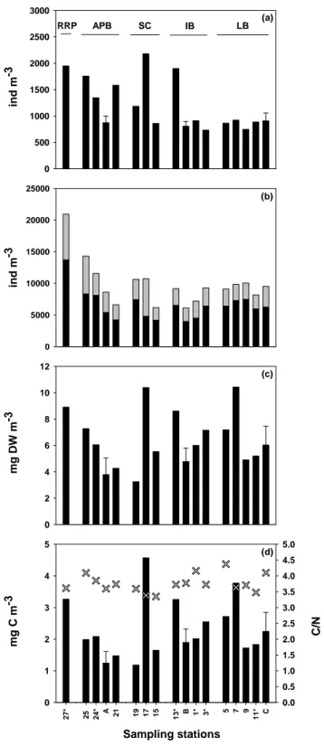
3.2 Zooplankton abundance and biomass distribution Zooplankton abundance in the upper 200 m layer estimated from the microscope counts (Fig. 2a) varied over the five geographic areas (RRP, APB, SC, IB and LB), with values (mean ± sd) of 1948, 1286 ± 409, 1407 ± 687, 1031 ± 492

and 872 ± 93 ind m−3, respectively. No significant

spa-tial differences were found between these five areas (Anova,

p >0.05). However, the general trend showed higher abun-dances in the western basin than in the eastern basin. Open water stations located in the western basin presented signifi-cantly (p < 0.05) higher abundance than those of the LB, but not to those in the entire eastern basin, due to the high abun-dance at station 13 (1901 ind m−3). Abundance was higher at the stations located in coastal regions (st. 27) and in the centre of the SC (st. 17) than in open water, with the low-est abundance located at station 3 (732 ind m−3). As for the total abundance pattern, nauplii and small copepods abun-dance did not show any significant differences between the five geographic areas (p > 0.05) (Fig. 2b). Nevertheless, at the basin scale, only small copepods abundance presented a significant higher abundance (p < 0.05) in the western basin (4450±2035 ind m−3₎_{than in the eastern basin (2627±340).}

In addition, in the western basin, a clear northward increase in both the nauplii and small copepods abundance with val-ues ranging from 20 929 (st. 27) to 6620 ind m−3(st. 21) was observed while it was not clear for the total abundance.

Zooplankton biomass (mg DW m−3₎_{was weakly but}

sig-nificantly correlated with abundance (ind m−3₎_(R2₌_0.298,

n =20, p < 0.01). Biomass displayed large spatial variabil-ity, with the values ranging from 3.2 mg DW m−3(st. 19) to 10.4 mg DW m−3(st. 17), equivalent to 1.2 to 4.6 mg C m−3 and 0.33 to 1.35 mg N m−3, respectively (Fig. 2c, d). Sta-tion 7 displayed a low abundance but a rather large biomass, which can be explained by the presence of large amphipods. A clear increase of DW biomass occurred northward in the APB (st. 21 to st. 27), but no clear pattern was observed in the other regions. In addition, no significant spatial differ-ences were found between the five geographic areas (Anova,

p >0.05). Mean zooplankton carbon and nitrogen contents represented 36.3 ± 3.7 % and 9.6 ± 1.2 % of the DW respec-tively. Zooplankton C/N ratio was fairly constant (mean: 3.78 ± 0.29) with values ranged from 3.35 to 4.37 at station 15 and 5, respectively.

3.3 Metazooplankton community composition and distribution

Over 74 taxa were identified from net tows during this study (Table 2) with 56 genera/species of copepods, 6 taxa of meroplankton and 12 taxa of holoplankton. Nauplii were present in the net samples but this technique, even when us-ing a 120 µm mesh net, did underestimate their real abun-dance, which was confirmed by the comparison with the in-tegrated abundance obtained with the Niskin bottle sampling

(7)

2164 A. Nowaczyk et al.: Distribution of epipelagic metazooplankton 0 500 1000 1500 2000 2500 3000 0 5000 10000 15000 20000 25000 0 2 4 6 8 10 12 27* 1 25 24* A 21 2 19 17 15 3 13* B 1* 3* 4 5 7 9 11* C 0 1 2 3 4 5 0.0 0.5 1.0 1.5 2.0 2.5 3.0 3.5 4.0 4.5 5.0 Sampling stations C/ N mg C m -3 ind m -3 ind m -3 mg DW m -3 RRP APB SC IB LB (a) (b) (c) (d)

Fig. 2. Spatial distribution of zooplankton integrated abundance ob-tained by net sampling (a) and by Niskin bottle (b) including nauplii (black) and small copepods (grey), biomass as dry weight (c) and as carbon (d) with C/N ratio (cross). Mean and standard deviation for stations A, B and C. (∗) night sampling. See text for details on the five Mediterranean areas.

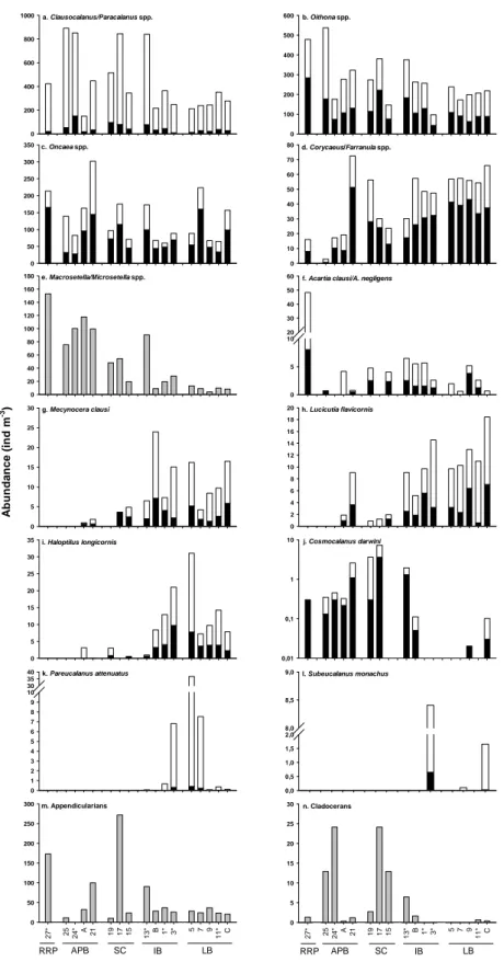
(see Sect. 3.4) and were given in Table 2 for information pur-pose only. Copepods represented 90.4 ± 3.0 % of total meta-zooplankton abundance and were dominated by 4 taxa: Clau-socalanus/Paracalanus spp., Oithona spp., Oncaea spp. and Macrosetella/Microsetella spp. which represented ∼80 % of the copepod community. The three first taxa were evenly dis-tributed along the transect but presented a local higher abun-dance (Fig. 3a, b, c), whereas Macrosetella/Microsetella spp. were 7 times more abundant in the western than in the eastern Mediterranean Sea (Fig. 3e). Euterpina acutifrons and mero-planktonic larvae were very common in neritic and coastal waters (e.g. st. 17 and 27 in Table 2). With the exception of one or two stations, Corycaeus/Farranula spp. and On-caea spp. populations were the only taxa dominated by adult stages (50 to 80 %).

Less abundant copepod species also displayed interesting geographical distribution. The genera Corycaeus/Farranula and Calocalanus spp. were less abundant in a large part of the western basin (Fig. 3d and Table 2). Mecynocera clausi, Lucicutia flavicornis, Haloptilus longicornis, Pareucalanus attenuatus and Subeucalanus monachus (Fig. 3g, h, i, k, l respectively) were clearly characteristic species of the east-ern basin being absent or with a very low occurrence in the western basin. Acartia species were located throughout the Mediterranean Sea (Fig. 3f). However, A. clausi replaced A. negligens in the north part of the western Mediterranean (st. 27 and 25) and at station 19 (Table 2). The subtropical copepod species Cosmocalanus darwini (Fig. 3j) was found in the two basins and is reported here for the first time in the Mediterranean Sea. Both adult and copepodite stages were collected.

Non-copepod holoplanktonic species, mainly appendic-ularians, ostracods, pteropods and chaetognaths, made up 9.3 ± 2.0 % of the metazooplankton abundance while mero-planktonic species were scarce (1.0 ± 1.4 %) except at the RRP (4.3 %). Cladocerans (Fig. 3n) were absent in the cen-tral sector of the eastern basin. Appendicularians (Fig. 3m) were 3 to 10 times more abundant at stations 27 and 17 than in the rest of the transect. It is also interesting to note that station C presented a high abundance (up to 11.6 ind m−3) of echinoderm larvae (Asteroidae).

Spatial impact of the mesoscale features, the anticyclonic gyres, when compared to the neighbouring stations was

more or less obvious (see Table 2 and Fig. 3).

Clauso-calanus/Paracalanus spp. were 2 to 4 time less abundant at stations A and B than at the adjacent stations, and only 1.5 less abundant at station C than at station 11. Mecynocera clausi and Corycaeus/Farranula spp. were on the other hand more abundant in the gyres than in the neighbouring stations especially obvious for the gyre B and C.

(8)

A. Nowaczyk et al.: Distribution of epipelagic metazooplankton 2165 0 50 100 150 200 250 300 350 0,01 0,1 1 10 0 100 200 300 400 500 600 0 10 20 30 40 50 60 70 80 0 20 40 60 80 100 120 140 160 180 0 5 10 20 30 40 50 60 0 2 4 6 8 10 12 14 16 18 20 0 5 10 15 20 25 30 35 0 1 2 3 4 5 6 7 8 9 10 30 35 40 27* 1 25 24* A 21 2 19 17 15 3 13* B 1* 3* 4 5 7 9 11* C 0 50 100 150 200 250 300 27* 1 25 _24* A 21 2 19 17 15 3 _13* B 1* 3* 4 5 7 9 11* C 0 5 10 15 20 25 30 c. Oncaea spp. d. Corycaeus/Farranula spp. e. Macrosetella/Microsetella spp. j. Cosmocalanus darwini i. Haloptilus longicornis

f. Acartia clausi/A. negligens

h. Lucicutia flavicornis n. Cladocerans m. Appendicularians b. Oithona spp. 0 5 10 15 20 25 30 0 200 400 600 800 1000 0,0 0,5 1,0 1,5 2,0 8,0 8,5 9,0 a. Clausocalanus/Paracalanus spp. g. Mecynocera clausi

k. Pareucalanus attenuatus l. Subeucalanus monachus

A bund a n c e ( ind m -3) RRP APB SC IB LB RRP APB SC IB LB

Fig. 3. Spatial distribution of the important zooplankton species across the Mediterranean transect: (a) Clausocalanus spp. and Paracalanus spp., (b) Oithona spp., (c) Oncaea spp., (d) Corycaeus spp. and Farranula spp., (e) Macrosetella spp. and Microsetella spp., (f) Acartia

clausi and Acartia negligens, (g) Mecynocera clausi, (h) Lucicutia flavicornis, (i) Haloptilus longicornis, (j) Cosmocalanus darwini, (k) Pareucalanus attenuatus, (l) Subeucalanus monachus, (m) Appendicularians and (n) Cladocerans. Copepodit (white), adult (black) and

undifferentiated (grey) stages. (∗) night sampling. Mean for stations A, B and C between day and night sampling. Note: logarithmic scale in panel (j).

(9)

2166 A. Nowaczyk et al.: Distribution of epipelagic metazooplankton

Table 2. Mean integrated abundance (± standard deviation) in the upper 200 m depth of total zooplankton, copepods, other holoplankton and meroplankton and percentage abundance of the major species and taxa within each category, for the different regions. Unidentified copepods and copepods <0.1 % were grouped as other copepods. Amphipods, isopods and gelatinous larvae were grouped as others.

Taxa Symbole Rhˆone Algero Sicily Ionian Levantin Algero Ionian Levantin

river Provencal channel basin basin Provencal eddy eddy

plume basin eddy

Total (ind m−3) 1948 1561 ± 205 1407 ± 687 1181 ± 630 855 ± 75 872 ± 129 806 ± 92 906 ± 151

Copepods (ind m−3) 1636 1457 ± 229 1230 ± 519 1073 ± 570 771 ± 83 773 ± 110 742 ± 74 828 ± 134

Other holoplankton (ind m−3) 228 102 ± 107 173 ± 184 107 ± 59 81 ± 19 90 ± 28 60 ± 20 69 ± 13

Meroplankton (ind m−3₎ _83.6 _{2.4 ± 3.7} _{3.6 ± 1.9} _{1.3 ± 1.1} _{2.7 ± 1.8} _{9.4 ± 9.2} _{4.0 ± 1.7} _{9.4 ± 4.4} Nauplii∗(ind m−3) 105 67 ± 54 92 ± 35 128 ± 128 74 ± 18 64 ± 18 100 ± 15 67 ± 7 Copepods (%) 84.0 93.3 87.4 90.8 90.2 88.6 92.1 91.4 Clausocalanus/Paracalanus spp. ClPa 21.7 46.8 40.4 41.0 30.6 17.1 26.9 30.5 Oithona spp. Oi 24.6 22.1 19.0 20.6 23.8 31.7 32.6 24.1 Oncaea spp. On 10.9 11.2 8.1 9.0 12.9 18.6 8.4 17.3 Macrosetella/Microsetella spp. MiMa 7.9 5.9 2.9 3.9 1.0 13.5 1.1 0.9 Corycaeus/Farranula spp. CoFa 0.8 2.0 2.6 3.6 6.6 2.2 7.1 7.3

Acartia clausi Acl 2.5 <0.1 0.1 0.0 0.0 0.0 0.0 0.0

Acartia negligens Ane 0.0 <0.1 0.1 0.4 0.3 0.5 0.7 0.1

Calanus helgolandicus Che <0.1 0.1 0.0 0.0 0.0 <0.1 0.0 0.0

Calocalanus pavo Cpa 0.0 0.0 0.4 1.3 0.9 0.0 0.4 0.5

Calocalanus spp. Ca 0.4 0.4 1.0 2.6 2.5 1.5 4.1 2.3

Candacia spp. Cd 0.1 <0.1 0.1 0.1 0.1 <0.1 <0.1 <0.1

Centropages typicus Cty 0.2 0.3 1.4 <0.1 0.0 0.0 0.0 0.0

Cosmocalanus darwini Cda <0.1 0.1 0.3 0.1 <0.1 <0.1 <0.1 <0.1

Ctenocalanus vanus Cva 2.1 0.0 0.6 0.8 0.8 0.0 0.0 0.0

Eucalanus hyalinus Ehy 0.0 0.1 <0.1 <0.1 <0.1 <0.1 0.0 0.0

Euchaeta spp. 0.2 0.1 0.1 0.2 <0.1 <0.1 <0.1 <0.1

Euterpina acutifrons Eac 4.1 0.0 0.1 0.4 0.0 0.0 0.0 0.0

Haloptilus spp. 0.0 <0.1 0.1 1.0 1.8 0.4 1.0 0.9

Lucicutia spp. 0.0 0.2 0.1 0.9 1.3 0.2 0.7 2.1

Mecynocera clausi Mcl 0.0 <0.1 0.2 0.8 1.1 0.1 3.0 1.8

Mesocalanus tenuicornis Mte <0.1 <0.1 0.0 <0.1 0.0 <0.1 <0.1 0.0

Nannocalanus minor Nmi 3.3 0.7 5.5 0.0 0.3 0.4 1.3 0.0

Neocalanus gracilis Ngr 0.0 <0.1 <0.1 0.2 0.1 0.1 0.1 <0.1

Pareucalanus attenuatus Pat 0.0 0.0 0.0 0.2 1.3 0.0 <0.1 <0.1

Pleuromamma abdominalis Pab 0.0 0.2 0.0 0.1 <0.1 0.2 <0.1 <0.1

Pleuromamma gracilis Pgr 0.6 0.1 0.2 0.4 0.1 0.4 0.1 <0.1

Scolecithricella spp. Sa 0.4 0.0 0.2 0.2 <0.1 0.0 0.6 0.3

Scolecithrix spp. Sx 0.0 0.0 <0.1 0.2 0.8 0.0 0.1 0.4

Spinocalanus spp. Sp 0.6 <0.1 0.8 <0.1 0.3 <0.1 0.2 0.1

Subeucalanus monachus Smo 0.0 0.0 0.0 0.2 <0.1 0.0 0.0 0.0

Temora stylifera Tst <0.1 <0.1 <0.1 0.3 0.3 0.0 0.0 0.1 other copepods 3.5 3.0 3.0 2.3 3.1 1.7 3.7 2.7 Other holoplankton (%) 11.7 6.6 12.3 9.1 9.5 10.3 7.4 7.6 Appendicularians AP 8.9 2.4 7.2 4.3 3.3 3.7 3.6 2.3 Chaetognaths CH 0.2 0.5 0.6 1.9 1.3 1.0 0.6 0.4 Cladocerans CL 0.1 0.8 0.9 0.2 <0.1 <0.1 0.2 <0.1 Doliolids DO 0.0 <0.1 0.0 <0.1 0.3 0.0 0.0 0.0 Euphausiids/Mysids EU MY 0.6 <0.1 0.1 0.1 <0.1 0.1 0.1 <0.1 Ostracods OS <0.1 2.3 0.8 1.2 3.0 3.7 1.4 2.7 Polychaetes PO 0.5 0.3 0.1 0.4 0.3 0.8 0.1 0.2 Pteropods PT 1.0 0.2 2.0 0.5 1.1 0.6 1.3 0.6 Salps SA <0.1 0.0 0.4 0.1 0.0 <0.1 <0.1 <0.1 Siphonophores SI 0.4 <0.1 0.2 0.3 0.1 <0.1 0.1 0.9 Others <0.1 <0.1 <0.1 0.1 0.1 0.4 <0.1 0.4 Meroplankton (%) 4.3 0.2 0.2 0.1 0.3 1.1 0.5 1.0 Decapod larvae DE 0.1 0.1 <0.1 0.0 <0.1 0.0 <0.1 <0.1 Echinoderm larvae EC 0.8 <0.1 <0.1 0.0 0.1 0.0 0.3 1.0 Fish eggs 0.1 <0.1 <0.1 <0.1 <0.1 <0.1 <0.1 <0.1 Fish larvae FI <0.1 <0.1 <0.1 <0.1 0.1 0.1 <0.1 <0.1 Jellyfishes JE 0.2 <0.1 0.1 0.1 <0.1 0.9 0.1 <0.1 Lamellibranch larvae LA 3.1 0.1 0.1 0.0 0.1 0.1 <0.1 0.0

(10)

0 40 100 120 200 140 160 180 80 60 20 0 40 100 120 200 140 160 180 80 60 20 0 40 100 120 200 140 160 180 80 60 20 27 26 25 24 23 A 22 21 20 19 18 17 16 15 14 13 12 B 1 2 3 4 5 6 7 8 9 10 11 C 0.2

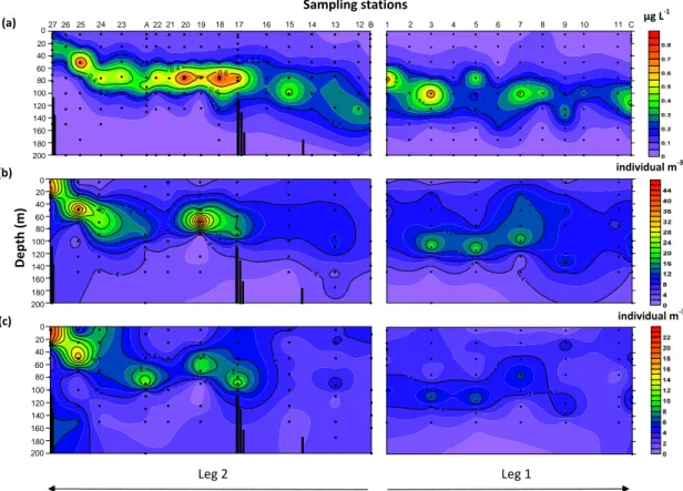
Fig. 4. Spatial distribution of chlorophyll-a concentration (a), copepods nauplii (b) and small copepods (c) within the upper 200 m layer across the Mediterranean Sea. Bottom depth in black. (b) (c) Depth (m) individual m‐3 Leg 1 Leg 2 (a) Sampling stations individual m‐3 µg L‐1

Fig. 4. Spatial distribution of chlorophyll-a concentration (a), copepods nauplii (b) and small copepods (c) within the upper 200 m layer across the Mediterranean Sea. Bottom depth in black.

3.4 Discrete sampling

The discrete depth sampling within the top 200 m collected small-sized copepods (<1 mm) and nauplii. The community of small copepods was composed of adult and copepodite stages of Oithona spp., Oncaea spp., Corycaeus/Farranula spp., Macrosetella/Microsetella spp., and copepodite stages of Clausocalanus/Paracalanus spp. Distinct spatial patchi-ness was observed in the distribution of both nauplii and small copepods throughout the Mediterranean Sea (Fig. 4). The depth of the maximum nauplii density matched that of small copepods for most stations with the exception of sta-tions 7 and 24. An eastward deepening of the depth of the highest abundance was observed from 25 m to 90 m in the western basin and from 100 m to 135 m in the eastern basin. Nauplii abundance was integrated over the upper 200 m ex-cept at st. 17 and 27 were depth range was limited to 100 m. Integrated abundance ranged from 4177 ind m−3 (st. 15) to 13 729 ind m−3(st. 27). It was 1.4 (st. 24) to 3.1 (st. 7) times higher than that of small copepods. The eastern basin showed an overall lower integrated abundance than the western basin and the SC for both nauplii and small copepods. Integrated values of nauplii and small copepods obtained using bottles sampling were 104 times and 4 times higher, respectively, than for samples collected with nets.

3.5 Zooplankton size structure

The automatic recognition system ZooScan (ZC) and the dis-secting microscope (MC) (Fig. 5) showed a significant lin-ear regression with ZC = 0.50 MC + 169.93 (R2=0.69, p < 0.001, n = 20). The lower detection limit for the ZooScan is 300 µm ECD, which led to an underestimation of the total number of organisms counted by ∼ 33±15.9 % (correspond-ing to 35.4 ± 14.9 % when nauplii were computed) when compared to the microscope technique. This underestima-tion corresponded to the fracunderestima-tion <300 µm ECD equivalent to a copepod with a total length of 500 µm. No clear pat-tern between the five geographic areas or between the west-ern and eastwest-ern basins were found for this single size frac-tion (p > 0.05). Nevertheless, the overall spatial distribu-tion of the metazooplankton abundance was similar between the two methods (Figs. 2a and 6). Biovolume (ZooScan de-terminations, data not shown) and biomass (Fig. 2c) also

shown similar spatial variations. Abundance and NB-SS

slopes (Fig. 6) did not show any clear relationship between the five geographic areas (p > 0.05). Nevertheless, the NB-SS slopes showed clear basin scale differences, with signif-icantly lower slope in the eastern basin (IB + LB) than in the western basin (APB) (p = 0.032), indicating a higher relative abundance of large organisms (>2 mm; such as

(11)

2168 A. Nowaczyk et al.: Distribution of epipelagic metazooplankton 0 500 1000 1500 2000 2500 0 500 1000 1500 2000 2500

Fig. 5. Comparison between microscope and ZooScan counts for all stations sampled with the

Bongo net.

ZooScan counts (ind m

-3)

y = x

Microscope counts (ind m-3)

Fig. 5. Comparison between microscope and ZooScan counts for all stations sampled with the Bongo net.

Haloptilus longicornis, Pareucalanus attenuatus and Subeu-calanus monachus) (Fig. 3i, k, l).

3.6 Day-night variation

At the three long-stay stations, significant higher abundance (∼17 %; p < 0.001) and biomass (∼40 %; p < 0.001) of or-ganisms >300 µm ECD observed at night highlighted the impact of the diel vertical migration on the structure of the community (Fig. 7). This increase was mainly explained by medium (500–1000 µm) and large-sized (>1000 µm) or-ganisms. Several specific taxa displayed higher night abun-dance within the upper 200 m. This included the copepods Euchirella messinensis and Neocalanus gracilis (p < 0.05), Pleuromamma abdominalis and P. gracilis (p < 0.01), as well as other taxa such as euphausiids, fish larvae (p < 0.001), pteropods and doliolids (p < 0.05).

The C/N ratio was overall stable (3.82 ± 0.26, n = 21) but decreased slightly during the night in spite of there being no significant difference between day and night samples. 3.7 Relationships between metazooplankton and

environmental parameters

No significant correlations between the different physico-chemical variables (temperature, salinity and oxygen) and the net metazooplankton abundance or biomass were found, while abundance of nauplii and small copepods from discrete samples were significantly correlated with oxygen level (Ta-ble 3). All metazooplankton parameters – both integrated and discrete data – were strongly correlated with chlorophyll-a concentrations (Fig. 8). Discrete abundance of nauplii and small copepods was strongly correlated with nanophyto-plankton, diatoms and POP concentrations. PON concentra-tion was the only variable showing a significant relaconcentra-tionship with both the net and discrete metazooplankton data.

27* 1 2524* A 21 2 19 17 15 3 13* B 1* 3* 4 5 7 9 11* C 0 250 500 750 1000 1250 1500 1750 2000 -2.0 -1.8 -1.6 -1.4 -1.2 -1.0 -0.8 -0.6

Fig. 6. Spatial distribution of mesozooplankton abundance (vertical bar) from the ZooScan counts and values of NB-SS slope (dark cross) along the BOUM transect. Mean values for stations A, B and C between day and night sampling. (*) night sampling. See text for details on the 5 regions. RRP APB SC IB LB Abundance (ind m ‐3 ) NB ‐SS slope Sampling stations

Fig. 6. Spatial distribution of mesozooplankton abundance (verti-cal bar) from the ZooScan counts and values of NB-SS slope (dark cross) along the BOUM transect. Mean values and standard devia-tions for stadevia-tions A, B and C between day and night sampling. (∗) night sampling. See text for details on the 5 regions.

Chlorophyll-a was included in all multiple regression models for biomass and integrated or discrete abundance (Ta-ble 4). Nanoplankton were selected as an explanatory vari-able in the model for integrated metazooplankton abundance as well as heteroflagellates in the models for integrated abun-dance of nauplii (HNF > 10 µm) and small copepods (total HNF).

The first factorial plane of the co-inertia analysis explained 69 % of the variance, with 52 % by the first axis. In both systems (“Environment” and “Zooplankton”), the three same groups of stations were observed (Fig. 9). Besides, the seg-regation obtained with the MDS analysis, based on the ob-servation scores of the 2 first axes of both systems, showed the same grouping (not shown). The first group was com-posed of all stations located in the western basin, except for st. A, and the western stations in the Sicily Channel (st. 19 and 17). The second group comprised all the stations lo-cated in the eastern basin except for st. 13. The third group was composed of the eastern station in the SC (st. 15), the eastern station in the IB (st. 13) and the anticyclonic gyre A. The first group was characterized by high values of nutri-ents, chlorophyll-a, nanophytoplankton and ciliates (Fig. 9a) and the second group by elevated temperature and salinity and high diatoms concentration. In the “Zooplankton” sys-tem, the first group was mainly identified by the copepods A. clausi, C. typicus and Calanoides carinatus while the sec-ond group by the copepods A. setosus, L. squilimana and H. longicornis (Fig. 9c, d). In both systems the third group of stations occupied an intermediate position on the factorial plane. Other taxa (appendicularians, pteropods, polychetes, the calanoid copepods Clausocalanus/Paracalanus and the cyclopoid and poecilostomatoid copepods Oithona and On-caea) were located near the barycentre. The relationship be-tween the normalized coordinates of the stations on the first

(12)

Table 3. Simple correlation analysis between zooplankton parameters and environmental factors: significance degree of p values. Integrated water column zooplankton abundance (ind m−3)and biomass (mg DW m−3)were obtained from net sampling (n = 20); discrete abundance of nauplii and small copepod (ind m−3)was issued from Niskin bottles (n = 111 to 140).

Abundance

Variable Symbole Net Biomass Net Total Integrated Discrete depths Small copepods Nauplii Small copepods Nauplii Temperature TEMP ns ns ns ns ns ns Salinity SAL ns ns ns ns ns ns Oxygen OXY ns ns ns ns ∗∗∗ ∗∗∗ HNF 2–5 µm HNF2 ns ns ns ns ns ns HNF 5–10 µm HNF5 ns ns ns ns ∗ ∗∗ HNF >10 µm HNF10 ns ns ns ∗∗ ns ns HNF total HNFT ns ns ∗ ns ns ∗∗ Nanophyto. NANO ns ∗∗∗ ns ns ∗∗ ∗∗∗ Diatoms DIAT ns ns ns ns ∗∗∗ ∗∗∗ Chlorophyll-a CHL ∗∗ ∗∗∗ ∗∗∗ ∗∗ ∗∗∗ ∗∗∗ Ciliates CIL ns ns ns ns ∗ ∗

Part. Org. Phos. POP ns ∗ ns ns ∗∗∗ ∗∗∗ Part. Org. Nitr. PON ∗ ns ∗ ∗ ∗∗∗ ∗∗∗ N/P particular Np/Pp ns ns ns ns ns ns

∗_{= p < 0.05;}∗∗_{= p < 0.01;}∗∗∗_{= p < 0.001, underlined stars mean negative correlation; ns: not significant.}

axis of both systems (“Environment” and “Zooplankton”) which reflects the degree of association between zooplank-ton and environment was highly significant (R2=0.89).

4 Discussion

4.1 Pattern of metazooplankton abundance and biomass along the BOUM transect

Zooplankton abundance values recorded, when using 120 µm bongo nets, during the BOUM transect, were 4 to 8 times higher than in previously published studies (Mazzocchi et al., 1997; Siokou-Frangou 2004; Gaudy et al., 2003; Pasternak et al., 2005; Riandey et al., 2005), whereas biomass were of the same magnitude. Strong discrepancies with previously recorded abundance may arise from (1) the use of different sampling mesh-size (120 µm during BOUM and >120 µm in all previous studies) and (2) differences in sampling peri-ods. Mesh size is a very important factor in the evaluation of metazooplankton abundance (Calbet et al., 2001; Turner, 2004). Zervoudaki et al. (2006) reported in a frontal area of the Aegean Sea, an increase of 2 to 20 times in abun-dance when smaller organisms (45–200 µm) were consid-ered. The most pronounced differences were observed for copepod nauplii, copepodites and adults of small organisms such as Clausocalanus/Paracalanus spp., Oithona spp., On-caea spp. and Macrosetella/Microsetella spp. Therefore it is clear that abundance is significantly higher when sampling is

performed with a 80 µm mesh size, but concomitant increase in biomass is not obvious (Thibault et al., 1994; Gaudy et al., 2003) probably due to the fact that small organisms have a low specific weight. According to the seasonal pattern of zooplankton production in temperate oceanic areas (Harvey, 1955), our abundance should be intermediate between maxi-mum late spring values and vernal minimaxi-mum values. Never-theless, for the seasonal period (June–July), our values (700– 2500 ind m−3)recorded in the 0–200 m layer with a 120 µm net were higher than that of Siokou-Frangou (2004; 50–900

ind m−3)recorded in the upper 100 m with a 200 µm mesh

net. This discrepancy highlights the difficulty when compar-ing different zooplankton datasets and the lack of common protocols.

The present work contributed to widening the characteri-zation of the zooplankton distribution in the Mediterranean

Sea. Our synoptic survey through the western and

east-ern basins confirms the eastward decrease of zooplankton abundance that has already been reported during other trans-Mediterranean surveys (Mazzocchi et al., 1997; Dolan et al., 2002; Siokou-Frangou, 2004; Minutoli and Guglielmo, 2009). In contrast, the biomass distribution did not show any large scale trend with average (∼6.3 mg DW m−3)and

max-imal (∼10.4 mg DW m−3) values similar between regions,

in agreement with biomass data compilations for various Mediterranean regions (Champalbert, 1996; Alcaraz et al., 2007; Siokou-Frangou et al., 2010). The apparent paradox between the trend in abundance and no trend in biomass might be explained by difference in size-spectra between the

(13)

2170 A. Nowaczyk et al.: Distribution of epipelagic metazooplankton 0 100 200 300 400 500 600 700 800 0 100 200 300 400 500 600 700 800 0 1 2 3 4 0 100 200 300 400 500 600 700 800 0 1 2 3 4 0 1 2 3 4 0 1 2 3 4 5 13/7 14/7 15/7 16/7 0 1 2 3 4 5 3/7 4/7 5/7 6/7 0 1 2 3 4 5 26/6 27/6 28/6 29/6

Fig. 7. Impact of sampling time (day: white; night: black) on zooplankton abundance integrated in the upper 200 m (ZooScan counts) (a, b, c), carbon biomass (d, e, f) and C/N ratio (g, h, i) at stations A, B and C.

Ind m ‐3 mg C m ‐3 C/N

Station A Station B Station C

Sampling dates

a. b. c.

g. _h.

d. e. f.

i.

Fig. 7. Impact of sampling time (day: white; night: black) on zooplankton abundance integrated in the upper 200 m (ZooScan counts) (a, b, c), carbon biomass (d, e, f) and C/N ratio (g, h, i) at stations A, B and C.

eastern and western basins. The presence of a few dominant large species, such as Haloptilus longicornis, Pareucalanus attenuatus and Subeucalanus monachus in the eastern basin, or the large amphipod Phronima sedentaria at station 7 could explain high local biomass. For example, the contribution of the three large copepod species to the total biomass was es-timated, using length-weight relationship (Webber and Roff, 1995; Hopcroft et al., 2002) to be 1.7 % (st. 13), 24.3 % (st. 3) and 30.5 % (st. 5). Therefore, large organisms contributed to the low NB-SS slopes observed in the eastern basin (see Fig. 6). In contrast in the western basin, high abundance was linked with the predominance of small organisms such as On-caea spp. and Macrosetella/Microsetella spp. This higher abundance of small organisms was confirmed by the Niskin bottle sampling.

In the western basin metazooplankton and small copepods abundances as well as the total biomass displayed a North-South decreasing gradient. D’Ortienzo and Ribera d’Alcal`a (2009) reported also this clear north-south gradient in the lower trophic level (chlorophyll-a levels) with a “northern

blooming area”, an “intermittently-blooming central area” and a “non blooming area” in the south.

The high biomass and abundance variability between sta-tions potentially arises from day-night variasta-tions, because sampling was conducted at different times of the day. When comparing day-night samplings at the three long stay sta-tions, diel variation led to an increase of 17 % in term of abundance and over 40 % in term of biomass due to in-creasing numbers of medium and large organisms (>500 µm ECD) at night as already observed in studies dedicated to the diel migration (Andersen et al., 1998, 2001, 2004; Riandey

et al., 2005). Variability in zooplankton abundance and

biomass could also be explained by the 3 identified anticy-clonic gyres characterized by a clear downwelling (Moutin et al., 2011) with, as consequence, a deepening in nutrients (Pujo-Pay et al., 2011) and low phytoplankton and micro-zooplankton biomass (Christaki et al., 2011; Crombet et al., 2011). On the other hand, freshwater and terrestrial mineral input from the Rhˆone River (Cruzado and Vel´asquez, 1990) could explain high nutrient levels and high phytoplankton

(14)

Table 4. Equation parameters of the multiple linear regression mod-els using forward stepwise method explaining the zooplankton pa-rameters distribution. Integrated zooplankton abundance (ind m−3)

and biomass (mg DW m−3)were obtained from net sampling (n = 20); discrete abundance of nauplii and small copepod (ind m−3)

was issued from Niskin bottles (n = 111 to 140). Symbols of vari-ables are described in Table 3.

Beta Beta standard P-level error

Integrated nauplii abundance

R2=0.53; adjusted R2=0.47; F = 8.61; P = 0.003 Constant 3.63 0.08

HNF10 0.27 0.09 0.008 CHL 3.15 1.22 0.021 Integrated small copepods abundance

R2=0.57; adjusted R2=0.51; F = 9.82; P = 0.002 Constant 3.10 0.12

CHL 4.17 1.14 0.002 HNFT 0.32 0.14 0.039 Integrated metazooplankton abundance

R2=0.75; adjusted R2=0.71; F = 21.89; P < 0.001 Constant 1.87 0.3

NANO 0.37 0.14 0.016 CHL 3.4 1.48 0.036 Integrated metazooplankton biomass

R2=0.55; adjusted R2=0.49; F = 9.18; P = 0.002 Constant −19.84 6.77

CHL 6.24 1.52 <0.001 SAL 12.70 4.21 0.009 Discrete nauplii abundance

R2=0.56; adjusted R2=0.54; F = 31.51; P < 0.001 Constant −12.79 2.22

O2 5.58 0.86 <0.001 CHL 2.29 0.36 <0.001 TEMP 1.01 0.37 0.007 Discrete small copepods abundance

R2=0.32; adjusted R2=0.31; F = 17.97; P < 0.001 Constant 1.20 0.08

CHL 1.33 0.35 <0.001 PON 1.97 0.59 0.001

and metazooplankton biomass in the river plume area (st. 27), as already evidenced by Gaudy et al. (2003). Variability resulted also probably from local hydrodynamic conditions linked to the bottom topography. The station 17 was very shallow with bottom depth ∼100 m and presented typical characteristic of a coastal stations with high values of chloro-phyll, high abundance of metazooplankton and a neritic com-munity. This was also reported in other neritic areas of the western basin such as the Balearic Sea (Fernandez de Puelles et al., 2004, 2009). Station 13 located over the margin area

0.05 0.10 0.15 0.20 0.25 0.30 400 600 800 1000 1200 1400 1600 1800 2000 2200 2400 27 25 24 Ad An 21 19 17 15 13 Bd Bn 1 3 5 7 9 11 Cd Cn 0.05 0.10 0.15 0.20 0.25 0.30 2 4 6 8 10 12 27 25 24 Ad An 21 19 17 15 13 Bd Bn 1 3 5 9 11 Cd Cn

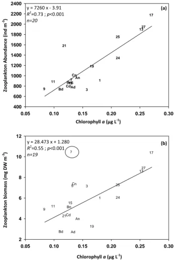
Fig. 8. Relationship between chlorophyll a concentration (µg L-1_{) and zooplankton abundance} (a) (microscope counts) and net zooplankton biomass (b) across the whole Mediterranean Sea. For A, B and C stations, day sampling (d) and night sampling (n). See table 1 and figure 1 for localization of stations. Note: st 7 biomass value was removed from the analysis.

y = 7260 x ‐ 3.91 R2_{=0.73 ; p<0.001} n=20 y = 28.473 x + 1.280 R2_{=0.55 ; p<0.001} n=19 (a) (b) Zoopl ank to n Abun dance (i nd m ‐3) Chlorophyll a (µg L‐1₎ Zoopl ank to n biom ass (mg DW m ‐3) Chlorophyll a (µg L‐1₎ 7

Fig. 8. Relationship between chlorophyll-a concentration (µg L−1)

and zooplankton abundance (a) (microscope counts) and net zoo-plankton biomass (b) across the whole Mediterranean Sea. For A, B and C stations, day sampling (d) and night sampling (n). See Table 1 and Fig. 1 for localization of stations. Note: st. 7 biomass value was removed from the analysis.

(slope between SC and IB) was also a site where local en-hancement can be observed.

Globally, the horizontal distribution of the metazooplank-ton in terms of abundance and biomass was mainly driven by the chlorophyll-a concentration (Tables 3, 4 and Fig. 9). Our study established empirical relationships (linear regres-sion) between metazooplankton abundance or biomass and chlorophyll-a concentration throughout the Mediterranean Sea. Chlorophyll-a (and subsequently zooplankton) distribu-tion was mainly driven by the eastward gradient in oligotro-phy which is a consequence of the thermohaline circulation and the nutrient inputs from rivers (Krom et al., 1991; Igna-tiades, 2005; Moutin and Raimbault, 2002; D’Ortenzio and Ribera d’Alcal`a, 2009).

In the Mediterranean Sea, the bulk of epipelagic mesozoo-plankton is generally concentrated within the upper 100 m (Scotto di Carlo et al., 1984; Weikert and Trinkaus, 1990;

(15)

2172 A. Nowaczyk et al.: Distribution of epipelagic metazooplankton a. Axis 1 (57%) -0.4 0.0 0.4 Ax is 2 ( 1 2 % ) -0.3 0.0 0.3 MLD CHL TEMP SAL OXY NANO DIAT HNF2 HNF5 HNF10 DIP POP PON DOP DON DIN Np/Pp CIL b. -2 0 2 -3 0 3 27 25 24 Ad An 21 19 17 15 13 Bd Bn 1 3 5 7 9 11 CdCn c. Axis 1 (57%) -3.2 0.0 3.2 A xis 2 (1 2% ) -3 0 3 Oi OnCoFa ClPa Ca Cpa Cca Cva Mcl Nmi Acl Ane Cty Lsq Lcl Lfl Lov Psp Sa Sx Sp Tst Cy Cp Eac MiMa Sa Che Cda Ehy Pat Smo Mte Ngr Aar Egi Ase Cd Ema Eme Hac Hlo Hmu Hpa Pab Pgr APCH JE DO SA SI POPT OxAt Pt AM DE EU MY IS CI CL OS EC LA FI d. -2 0 2 -3 0 3 27 25 24 Ad An 21 19 17 15 13 BdBn 1 3 5 7 9 Cd₁₁ Cn A xis 2 (1 2% ) Axis 1 (57%) Axis 1 (57%) Fig. 9. Co‐inertia analysis: plots of the environmental variables (a) and the stations (b) in the “Environment” system and plot of the taxa (c) and the stations (d) in the “Zooplankton” system. Circles corresponded to cluster group tested with non parametric MANOVA. Mixed Layer Depth (MLD), Aetideus armatus (Aar), Arietellus setosus (Ase), Calanoides carinatus (Cca), Clytemnestra spp. (Cy), Copilia spp. (Cp), Euaetideus giesbrechti (Egi), Euchaeta marina (Ema), Euchirella messinensis (Eme), Haloptilus acutifrons (Hac), H. longicornis (Hlo), H. mucronatus (Hmu), Heterorabdus papilliger (Hpa), Lubbockia squillimana (Lsq), Lucicutia clausi (Lcl), L. flavicornis (Lfl), L. ovalis (Lov), Phaenna

spinifera (Psp), Sapphirina spp. (Sa), Amphipods (AM), Cirriped larvae (CI), Isopods (IS), Oxygyrus/Atlanta spp. (OxAt) and Pterotrachea spp. (Pt). Other abbreviations as in Tables 2 and 3.

Fig. 9. Co-inertia analysis: plots of the environmental variables (a) and the stations (b) in the “Environment” system and plot of the taxa (c) and the stations (d) in the “Zooplankton” system. Circles corresponded to cluster group tested with non parametric MANOVA. Mixed Layer Depth (MLD), Aetideus armatus (Aar), Arietellus setosus (Ase), Calanoides carinatus (Cca), Clytemnestra spp. (Cy), Copilia spp. (Cp),

Euaetideus giesbrechti (Egi), Euchaeta marina (Ema), Euchirella messinensis (Eme), Haloptilus acutifrons (Hac), H. longicornis (Hlo), H. mucronatus (Hmu), Heterorabdus papilliger (Hpa), Lubbockia squilimana (Lsq), Lucicutia clausi (Lcl), L. flavicornis (Lfl), L. ovalis (Lov), Phaenna spinifera (Psp), Sapphirina spp. (Sa), Amphipods (AM), Cirriped larvae (CI), Isopods (IS), Oxygyrus/Atlanta spp. (OxAt) and Pterotrachea spp. (Pt). Other abbreviations as in Tables 2 and 3.

Brugnano et al., 2010) and mainly within the upper 50 m in both the eastern basin (Mazzocchi et al., 1997) and the Ligurian Sea (Licandro and Icardi, 2009). Here, the bulk of both nauplii and small copepods presented a patchy ver-tical distribution (down to 120 m) throughout the Mediter-ranean Sea, mainly driven by the deep chlorophyll maxi-mum (DCM) depth. Clear association between vertical dis-tribution of epipelagic mesozooplankton and DCM has pre-viously been shown during the summer stratified period (Al-caraz, 1985, 1988; Alcaraz et al., 2007; Sabat´es et al., 2007). Higher grazing activity by copepods is also often associated with DCM as demonstrated by increased phaeophorbide con-centration (Latasa et al., 1992). Here, the nauplii abundance vertical distribution showed a maximum matching the DCM except at a few stations where temperature at the maximum

nauplii concentration was ∼15◦_{C. The multiple regression}

analysis confirmed the combined effort in the search for the optimal food availability (DCM) and the best thermal condi-tions for development (Chinnery and Williams, 2004; Koski

et al., 2011). Nauplii and small copepod vertical distribu-tions were also correlated with oxygen, PON and POP, but these variables are indirectly linked to phytoplankton abun-dance through photosynthesis, respiration and organic com-position. Their distribution was also associated with het-erotrophic nanoflagellates and ciliates, suggesting a link with the microbial loop, which is known as a potential food source for small planktonic organisms (Calbet and Saiz, 2005; Hen-riksen et al., 2007). Horizontal distribution of the abun-dance of nauplii, small copepods and metazooplankton was correlated with the distribution of HNF >10 µm, total HNF and nanophytoplankton respectively. The affinity of nauplii for small motile prey such as HNF was evidenced experi-mentally by Henrikzen et al. (2007), that of small copepods for phytoplankton and microheterothrophs (Nakamura and Turner, 1997; Zervoudaki et al., 2007) and of metazooplank-ton for nanophytoplankmetazooplank-ton performed at different season of the year (Pinca and Dallot, 1995; Gaudy and Youssara, 2003; Alcaraz et al., 2007; Zervoudaki et al., 2007) is also well

(16)

known. Finally physical forcing can also affect vertical dis-tribution as shown by Andersen et al. (2001), with nauplii of copepods and euphausiid being influenced by a deepening of the mixed layer and a dilution of the phytoplankton biomass in the water column following a wind event.

4.2 Pattern of zooplankton assemblages in relation with environmental parameters

The zooplankton composition recorded during the BOUM transect was in general agreement with the published data on the Mediterranean Sea community (Siokou-Frangou et al., 1997, 2010; Gaudy et al., 2003; Pasternak et al., 2005; Riandey et al., 2005). The overall metazooplankton com-munity was dominated by copepods and especially by small size species (<1 mm). Clausocalanus/Paracalanus spp. and Oithona spp. were the dominant genera, as is generally ob-served (Gaudy et al., 2003; Peralba and Mazzocchi, 2004; Zervoudaki et al., 2007).

We found a clear distinction in taxonomic composi-tion between the western and the eastern basins mainly

driven by ecological characteristics. Several copepods

species showed a clear eastward pattern. For example,

Macrosetella/Microsetella spp., Acartia clausi and Cen-tropages typicus were more abundant in the western basin; while, Calocalanus pavo, Corycaeus/Farranula spp., Halop-tilus longicornis, Lucicutia flavicornis, Mecynocera clausi and Pareucalanus attenuatus were present mainly in the east-ern basin. The spatial distribution of most species reported here has been confirmed by Siokou-Frangou et al. (2010). Other taxonomic groups presented also a clear spatial pat-tern. Cladocerans were nearly absent from the eastern basin, which may be also explained by the difference in the sam-pling dates between the two basins (>2 weeks). Indeed, these organisms are known to display explosive growth over very short time-periods linked to their parthenogenetic repro-duction (Christou and Stergiou, 1998; Atienza et al., 2007, 2008). The distance to the coast could also explain local high abundance, such as in the Sicily Channel, of these organ-isms, known to have a neritic affinity (Fernandez de Puelles et al., 2007). These differences in the percentage contribu-tion of some important species to the whole copepod assem-blage might reflect differences in species biogeography, but might also be indicative of different associations between structural and functional features. In the co-inertia analy-sis (Fig. 9), the eastern basin was characterized by high di-atoms concentration associated with higher abundance, com-pared to other stations, of large-size herbivorous copepods i.e. Pareucalanus attenuatus (st. 5 and 7) and Subeucalanus monachus (st. 13) both restricted to the eastern basin. High abundance of these copepods also corresponded to hot spots of biogenic silicon dominated by the microphytoplankton Chaetoceros spp. in the eastern basin (Crombet et al., 2011). Subeucalanus monachus has already been reported in high abundance in the Rhodes cyclonic gyre where nutrients rich

waters have been upwelled leading to high phytoplankton biomass dominated by large diatoms (Siokou-Frangou et al., 1999). One novelty observed during the BOUM cruise is the presence of Cosmocalanus darwini reported for the first time in the Mediterranean Sea, both in the western and eastern basins. We found copepodites stages as well as females in-dicating the reproductive success of this species. However, it is difficult to conclude about its origin in the Mediterranean Sea. This species is common in the Red sea (Razouls et al., 2005–2011; web site) and is expected to undergo lesseptian dispersion but this species was found in lower abundance in the eastern basin than in the western basin.

On the other hand, the western basin was characterized by high nutrient concentrations, high abundance of nanophyto-plankton and small and medium (<1.5 mm prosome length) herbivorous/omnivorous copepods (i.e. Acartia clausi, Cen-tropages typicus, Euterpina acutifrons). The association of these small copepods species with nanophytoplankton-rich conditions has already been demonstrated in the Mediter-ranean (Pinca and Dallot, 1995; Gaudy and Youssara, 2003; Alcaraz et al., 2007; Zervoudaki et al., 2007).

Mesoscale hydrodynamic structures could also play an im-portant role in the variability of zooplankton abundance and community structure. Anticyclonic gyres displayed lower abundance of metazooplankton and less marked vertical dis-tribution than neighbouring stations where higher chloro-phyll concentration at the DCM was observed. These gyres showed a metazooplankton community characterized by lower Clausocalanus/Paracalanus (herbivorous) and more Corycaeus/Farranula spp. (omnivorous) that could reflect changes in food availability (increase in oligotrophy, lower chlorophyll concentration) (Legendre and Rassoulzadegan, 1995).

The position of station A in the co-inertia analysis is pe-culiar, highlighting the response of the zooplankton com-munity structure to the environmental forcing. Geograph-ically belonging to the western basin, the physical condi-tions prevailing at station A led to a different zooplankton composition (i.e. less Clauso/Paracalanus spp., and more Corycaeus/Farranula spp. and P. gracilis) than other stations in the APB; therefore station A emerged on the co-inertia analysis half way between its geographical group and the group where station B and C were located. Nevertheless, the gyre located at station C did not display a lower abundance and biomass than surrounding LB stations. Its functioning could be slightly different from the two other gyres resulting in stronger (0.441 µg L−1₎_{and deeper (120 m depth) DCM.}

Moreover, its location close to the Cyprus coast could explain the high abundance of echinoderm larvae through the aggre-gation effect of the gyre (Pedrotti and Fenaux, 1996). In-deed, these structures are known to affect mesozooplankton community structure and functioning (Youssara and Gaudy, 2001; Beaugrand and Iba˜nez, 2002; Isla et al., 2004; Riandey et al., 2005; Hafferssas and Seridji, 2010).