Does monetary poverty reflect caloric intake?

HAL Id: hal-01006496

https://hal.archives-ouvertes.fr/hal-01006496

Submitted on 16 Jun 2014

HAL is a multi-disciplinary open access

archive for the deposit and dissemination of

sci-entific research documents, whether they are

pub-lished or not. The documents may come from

teaching and research institutions in France or

abroad, or from public or private research centers.

L’archive ouverte pluridisciplinaire HAL, est

destinée au dépôt et à la diffusion de documents

scientifiques de niveau recherche, publiés ou non,

émanant des établissements d’enseignement et de

recherche français ou étrangers, des laboratoires

publics ou privés.

To cite this version:

I. Bocoum, S. Dury, J. Egg, J. Herrera, Y. Martin Prevel. Does monetary poverty reflect caloric

intake?. Food Security, Springer, 2014, 6 (1), p. 113 - p. 130. �10.1007/s12571-013-0318-0�.

�hal-01006496�

Does monetary poverty reflect caloric intake?

Ibrahima BOCOUM CIRAD, UMR MOISA, F-34398 Montpellier, France

IRSTEA, UMR ITAP, F-34000 Montpellier, France

Sandrine DURY CIRAD, UMR MOISA, F-34398 Montpellier, France Johny EGG INRA, UMR1110MOISA, F-34000 Montpellier, France

Javier HERRERA IRD, UMR DIAL, F-75000 Paris, France

Yves MARTIN-PREVEL IRD, UMR NUTRIPASS, F-34000 Montpellier, France

Corresponding author: Ibrahima Bocoum. Email: ibbocoum@gmail.com.

Abstract:

The use of expenditure surveys to measure food insecurity is widelydiscussed.In this study, we investigatefood insecurity in terms of monetary poverty. Using a Maliansurvey thatincorporatesexceptionally detailed information on food consumption, we estimate that 35% of the households are in a paradoxical situation,some poor households managing to cover their caloric requirements by eating cheap calories and some non-poor households not doing so because they consume expensive calories and/or face constraints such as the obligation to share meals with visitors and high expenditure on health care or transportation. These findings highlight precautions that need to be taken when measuring food insecurity through monetary income or expenditure indicators.

KEY WORDS: poverty, food insecurity, caloric intake, household surveys, Mali

1 Introduction

Estimating the number of people who are food insecure is an important monitoring issue for development and food security policies, as well as for monitoring the impacts of economic crises. However, there is no simple, universally accepted method forassessing the proportion of a population that is food-insecure,as Headey (2013) has recently demonstrated in hisassessment of the impact of the 2007/08 global food crisis. Since the 1970s, the FAO method, which refers to the global level of food availability, has been based on food balance sheets,assessed from macroeconomic data onproduction, trade, and consumption. Whilethis islegitimate at the international level, it is nonetheless criticized as an indicator of the number of people undernourishedat local levels (for instance Svedberg, 1999, 2000, 2002). This is because it is based on highly aggregated data and hardly explicit hypothesesof distribution among individuals and households.However, during the past two years, the FAO has deployed a great deal of effort to update the food availability data as well as the methodology used to estimate undernourishment (e.g. FAO WFP and IFAD 2012).Household surveys of certain countries have been used to assess more accurately the inequalities of food access within populations.While these changes have resulted in the revision downward of the number of undernourished and the finding that undernourishment has declined more strongly since 1990, the FAO acknowledges that important gaps in data and deficiencies in data quality remain. A more comprehensive picture of the food security situation in every country requires additional indicators(FAO WFP and IFAD 2012). Svedberg (1999 and 2002) recommends employing anthropometric indicators whereasHeadey (2013) proposes usingself-reporting indicators. Another alternative is to use food consumption and monetary poverty indicators obtained from Household Consumption and Expenditures Surveys (HCES) such as Living Standard Measurement Surveys (LSMS), mainly based on household expenditure recall.These surveys are conductedon a regular basis in most developing countries and encompass large representative samples of several thousand households.To our knowledge,surprisinglyfew authors (with the exception of Smith andSubandoro, 2007) have formally raised and investigated the question of whether these surveys could be used to assess and monitor food security at the household and national levels. This very recent trend hasbeen discussed both by global institutions and scientists.

Through joint initiatives, the World Bank and the FAO are currently trying to take stock from these household surveys. As a follow up to a meeting in 2010, the Committee on World Food Security (CFS) asked the FAO to revise its methodology for assessing undernourishment. One of the recommendations was to make more use of the large household surveys available in different countries. Discussions on this topic also took place at a workshop in Washington DC in April 2011 (“Monitoring,

Assessment,and Data Working Group of the Ten Year Strategy for the Reduction of Vitamin and Mineral Deficiencies”)1 and at an international symposium in Rome in January 2012 (“International Scientific Symposium on Food & Nutrition Security”).

The strengths and weaknesses of Household Consumption and Expenditure Surveys (HCES)were also recently discussed from a “nutrition community perspective” (Fiedler,2012) as a tool to assess dietary intake (e.g.Dopet al 2012) or to design nutritional intervention programs (Murphy et al. 2012). These authors comparedfood consumptiondata calculated from HCES (including purchases, self-consumption and gifts received, expressed in monetary units and converted into kilograms, and then into calories, nutrients, etc.) with other means to measure food consumption (for instance, 24-hour recall). In other words, they discuss the relevance of HCES from an external point of view, while we propose to discuss it from an internal one.Indeed, in the present paper, we put forwarda comparison of the level of household poverty, which is the main objective of these surveys, with their level of food consumption. We examine in detail the households that have inadequate food consumption though are not poor according to the monetary poverty indicator and, conversely, those that have adequate food consumption but are monetarily poor.

The overall objective of this paper is thus also to contribute to the debate on the opportunity of using existing HCES to assess the food insecurity status of a population. Here we chose to stick to the original purpose of these HCES (measuring and monitoring poverty through monetary indicators) because a huge part of the limited statistical capacities of poor countries, especially those under the Debt Initiative for the heavily indebted poor countries, is devoted to the calculation and monitoring of poverty using these HCES. The idea is to empirically verify whether this indicator of monetary poverty can be used as an indicator of food insecurity.

More precisely,using the national poverty assessment survey carried out in 2001 in Mali —whichis unique asit captured both food consumption (measured in quantities) and expenditures (measured in monetary units) — we compare the overlap between a poverty indicator and a food insecurity indicator (household caloric requirement). Certain HCES also include anthropometric indicators (in the case of Mali the 1988/89 budget and consumption survey and the 2001national poverty assessment survey). Given that these indicators only focus on children under five years old, we assume that they are less representative of the holistic situation of the household than caloric intake. However, a persistent deficit of caloric intake and poorperformance using anthropometric indicators are connected. Moreover, by considering the deficit of caloric intake as an indicator of food insecurity, our study is relevant for less developed countries where obesity problems do not exist or are rare.

The paper is structured as follows: after a brief review of the controversy in the scientific literature concerning the relationship between caloric intake and income/total expenditure,the study’s methodology, data, and econometric model are presented. The next sections present the descriptive and econometric results.Section 5 finally discusses the results.

2 Literature review: Relationship between caloricintake and income/total expenditure

The conventional view is that insufficient food consumption is linked to insufficient income (Strauss and Thomas 1995; Abdulai and Aubert 2004a, among others). We expect therefore that poor households are food insecure and wealthy households are food secure. But the research results on this topic vary by author and type of indicator employed. Many authors have investigated the relationship between income or total household expenditure (easier to measure) and food insecurity, particularly through the study of "Engel curves2" of calories or more sophisticated demand models. The majority of these works (Subramanian and Deaton 1996; Ohri-Vachaspatiet al 1998; Abdulai and Aubert 2004b) have concluded that an increase in households’ income or total expenditure would increase their consumption of calories. While these studies have strengthened the view that food insecurity (measured by caloric intake) is associated with low income, Behrman and Wolfe (1984), Behrman and Deolalikar (1987), and Bouis and Haddad (1992) have explained that an increase in a household’s income (including among the poorest) is not necessarily accompanied by extra consumption of calories. It

1_{The workshophas led to a special issue of Food and Nutrition Bulletin: Food and Nutrition Bulletin,}

vol. 33, no. 3, 2012.

2_{Engel, a nineteenth-centurystatistician,was interested inthe evolution ofbudget proportionsaccording} toincome.We are interested incaloric intake,but wesimplify it bysaying “Engel curve.”

depends on income elasticity for each food item.Staple foods are usually considered to be inferior goods while meat and other processed foods are often regarded asnormal or superior goods. Another explanation pointed out by Deaton and Dreze (2009) is an increase in food or calorie prices relative to the prices of others goods.

In India, Deaton and Dreze (2009) and Haddad (2009) have recently found that, despite rapid macroeconomic development — the growth of real incomes and the lack of anincrease for foodrelative to income —individuals’ caloricintakes declined between 1983 and 2004. These results are very troubling, as the authors themselves acknowledged. Finally, other studies (e.g.Baulch and Masset 2003; Darmon et al 2010) have comparedmonetary poverty and various food security indicators (nutritional status, individuals’ perceptions) andhave found that the connections between these indicators areweak.

3 Materials and methods 3.1 Data

The data used here comes from a national household survey carried out in 2001 with the support of the World Bank — the Malian Poverty Assessment Survey (DNSI 2004).Households were selected using a two-stage cluster sampling method: the enumeration area (EA) and the household (DNSI 2004). The 1998 census divided the Malian territory into 12,000 EAs containing roughly100 households each. For the survey, 750 EAs well distributed by region and rural/urban areas were randomly selected. Ten households were randomly selected from each EA, leading to an initial sample size of 7,500 households. Our analyses focused on a subsample of 4,952 households for which complete data were available and of which 3,121 were rural and 1,831 urban. The survey was conducted in four rounds between January and December 2001. The data collected concerned socio-economic characteristics, food and non-food expenditure statements, as well as the weights of food cooked and consumed in the households.Each round lasted one week during which the surveyors identified the weekly recurrent expenditure and the exceptional expenditure of the three previous months. Foods used in the preparation of various meals consumed at home were systematically weighed every day.

3.2 Empirical model

In this paper, we use caloric requirements as an indicator of food insecurity at the household level and compare it with an indicator of monetary poverty.. This comparison gives four possible situations: poor households with insufficient calories, non-poor households with sufficient calories (both expected), poor households with sufficient calories and non-poor households with insufficient calories (both unexpected and paradoxical).

After examining the proportions of households in each situation, we tried to identify factors that affected the relationship between monetary poverty and total caloric requirements. Thesewere the budget structure of households, the cost of the calories consumed, solidarity among households, education of households’ women, possession of non-monetary assets, demographic characteristics of households, geographical location and ethnicity.

We used a multinomial logistic regression model in which the different combinations of monetary poverty and food consumption outputs are explained by a set of regressors, namely households’ socio-demographic characteristics.The model is essentially empirical the selected explanatory variables reflecting households’ choices (cost of calories consumed, budget proportions) and demographic characteristics (region, ethnicity, environment, etc.).

The probability for a household of being in a particular situation can be written as follows:

= = | =_{1 + ∑}exp _exp

Where j=1,...,4 represents the situation in which the household is found (corresponds to one of the four modalities described above)

X is a vector of explanatory variables

is a vector of parameters associated with the explanatory variables

k is the baseline

The probability of being in a particular situation is considered in comparison with the probability of being in the base outcome and is written as:

= = + 1| =_{1 + ∑} 1_exp

The standard interpretation of the results of such a model consists in analysing factors that increase or decrease the probability of being in one situation with reference to a differentsituation. Suchan interpretation is not really convenient in our case given the high number of situations, all being not relatively interpretable to a unique situation of reference. Marginal effects of changes in explanatory variables on the probability = | were thus calculated using the method proposed by Chamberlain (Cahuzac and Bontemps 2008). These average marginal effects represent the variation in percentage points of the probability of being in a particular situation when an explanatory variable varies by a unit (quantitative variable) or 0-1 (dichotomous variable). Bartus (2005) considered this methodas being the most relevant. The validity of the multinomial logit model is based primarily on the hypothesis of the independence of alternatives. Testing this hypothesis consists ofchecking that removing one of the four modalities from the dependent variable does not have a significant impact on the estimated coefficients.

3.3 Construction of caloric intake and poverty indicators

The total expenditure used to calculate the monetary poverty indicator reflects the sum of the expenditure really incurred,plus the amount of self-consumed production. A monetary value was given to self-consumed production using unit values of purchased goods (expenditure divided by quantities). Median unit values were used in each region. These unit values are quite similar to the actual prices available. In addition, the expenditure concerning durable goods was excluded due to the lack of information on the duration of their depreciation. According to Subramanian and Deaton (1996), the exclusion of this type of expenditure is a standard procedure to minimize the statistical noise.

The poverty line was calculated for each region and type of area (rural or urban). Cost of calories corresponding to the average minimum caloric requirements in each zone (area or region) was estimated, based on an identical food basket containing the foods usually consumed in all regions. The result obtained corresponded to the food poverty line. This line thus depends in part on the structure of activities, age, and gender of individuals in each zone, which influence the minimum caloric requirements, and on the local prices of commodities included in the basket. To estimate the overall poverty line (also taking into account non-food requirements), households whose food expenditure was close to the food poverty line have been identified and their total average expenditure has been calculated.

Two techniques were tested(Bocoum 2011): one described by Pradhanet al. (2001) and another by Ravallion (1998). Different results were found (see Table A2). The incidence of monetary poverty in Mali oscillates between 50% and 61%, depending on the poverty line selected, but the regression results are not qualitatively different. Only the results of the lowest line (the most "optimistic") are presented here. To calculate the calories consumed for meals prepared and consumed inside the home,the weight of the food’s edible portion used for preparing daily meals was converted into calories using a Malian food composition table (Nordeide 1997). Leftovers and dishes given to other households were subtracted, while dishes received by the household were added to calculate the total amount of calories consumed daily inside the home. The amount of calories consumed outside the home by all household members was estimated and added to home consumption. The final total amount was then divided by the actual number of portions (number of people sharing the meals) to assess the household’s average daily food consumption in calories per capita.

Caloric requirements were calculated for each individual in each household from the basal metabolic rate according to gender, age, weight, height, and considering a medium physical activity level. The calculation method was that of Swindale and Ohri-Vachaspati (2005). Total energy requirement at the household level was calculated by dividing the average daily food consumption by the average requirement. Households not reaching 100% were classified as “with insufficient caloric intake” and those reaching 100% were classified as “with sufficient caloric intake”.

Box 1: Treatment of data outliers

Data outliers on the quantities used for the preparation of meals and expenses have been detected and treated as follows.The statistical distribution of each type of food (over a hundred) and each of the 39 expenditure categories in each stratum (urban or ruralarea, region, household size) were analysed. Information outliers were identified by defining “realistic”inter-quartile intervals around the median of distributions. Different intervals were tested before selecting the intervals [median + / -2 * (Q3-Q1)] for weighted quantities and [median + / -6 * (Q3-Q1)] for the different expenditure types that seemed to be the most effective given the results. The correction of outliers and missing data consisted of imputing the median value per capita of distribution in the region and the environment in question. These data entries were made for a total of fewer than 10% of observations, which limits the bias that such an action could potentially introduce. The fact remains that our data entry method has the potential effect of “centralizing”the data since we replacedextreme data, judged too weak or too strong, with a median value corresponding to a relatively “homogeneous” group (for the region, area, and household size). Given that this article highlights the extreme cases, it can be assumed that our data entry method has a reducing effect on them.

4 Results

4.1 Characteristics of households’budget and caloric consumption

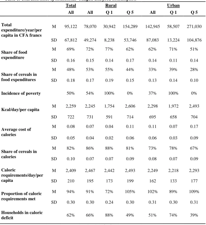
Table 1 and A1 show the different characteristics related to the mean household budget and caloric consumption. The total annual expenditure (excluding durable goods) per household amounted to a national average of 96,825 CFA francs (FCFA) — 79,577 FCFA and 145,197 FCFA in rural and urban areas respectively. The average rural income of 73,235 FCFA revealed by the more recent RuralStruc surveys3 (Samakéet al. 2008) supports our estimates. But, our estimates arebelow the figures published by DNSI (2004) using the same survey as us: respectively 169,334 FCFA, 129,012 FCFA, and 267,682 FCFA respectively at the national, rural and urban level.

Although our estimates do not take into account the durable goods (1.8% of householdbudget on average),the differencewith the above figures isprimarilydue to the data cleanings made from the raw data (see Box 1). Indeed, there were many outliers identified in collaboration with statisticians of the National Institute of Statistics of Mali that have been corrected by imputation.

Food expenditures represent on average 70% of the total expenditures (72% in rural areas and 62% in urban areas). Cereals represent almost 50% of the food expenditures (53% in rural areas and 33% in urban areas. The shares of food in terms of total expenditure, as well as the share of cereals within food expenditure decrease with increasing total expenditures, as the figures by quintiles of total expenditures show.This actually confirms respectively Engel’s and Bennett’s laws.

About 50% of Malians were below the poverty line (respectively 54% and 37% of rural and urban inhabitants). The figures, obtained from the analysis of a recent smaller and less detailed survey, show a slight decrease in these poverty incidences which were 44% at the national scale, 51% at the rural scale and 31% at the urban scale (Eozenouet al., 2013).The inequalities of total expenditure between the households were very high between the poorest quintile and the least poor quintile, but also within the quintiles.

Our estimates showed that the average caloric intake reached 2,259 kilocalories per day per person in Mali in 2001.It should be noted that this result is very close to that estimated by the FAO4 (2,390 kcal/day/person in 2001), indicating the relevancy of FAO’s assessment for this indicator at national scale.In our case, individual food consumption surveys were compiled, whereas the FAO estimate was made based on a food balance sheet from agricultural statistics and average consumption ‘norms.’ This closeness of the results surprised us given the complexity of the surveys and aggregation calculations in both cases, and tends to reinforce the two methodologies.

These surveys wereconducted with610farmsin 24villages in thedifferent production areasof Mali. 4_{The FAO website assessed on 25/03/2012.} http://www.fao.org/economic/ess/ess-fs/fs-data/ess-fadata/fr/

There is little difference between rural and urban inhabitants (respectively 2,245 and 2,298 kcal/day/person). In contrast, the poorest have a significantly lower caloric intake in both rural and urban areas.

The main sources of calories are cereals. They represent, on average, 82% of the total calories consumed. This share is higher in rural areas but decreases with increasing total expenditures.

The share of cereals in total consumption is closely related to the average cost of the calories consumed. Indeed, cereals represent the cheapest source of calories and a lower proportion of this type of food in the food basket is associated with a higher average cost of calories, but also with a more diversified diet.

On average, energy consumption reached 2,409 kilocalories/day/person at the national level (respectively 2,467 and 2,249 in rural and urban environments). Country-wide, Malians consume approximately 94% of their total energy requirement (i.e. calorie intake/average requirement): this is a mean of 91% in rural areas and 102% in urban areas. But this is a very incomplete picture because it ignores inequalities. Indeed, if this calculation is done at the household level, 62% of Malians appear in caloric deficit (66% in rural areas versus 51% in urban areas).

At the country level, and both in rural and in urban areas, the percentage of households in caloric deficit was higher than those that are poor. Moreover, even in the richest quintile of the population, the incidence of energetic deficit was high (between 40 and 50%).

Table 1. Characteristics of households’ budgets and food consumption

Total Rural Urban

All All Q 1 Q 5 All Q 1 Q 5

Total

expenditure/year/per capita in CFA francs

M 95,122 78,070 30,942 154,289 142,945 58,507 271,030 SD 67,812 49,274 8,238 53,746 87,083 13,224 104,876 Share of food expenditure M 69% 72% 77% 62% 62% 71% 51% SD 0.16 0.15 0.14 0.17 0.14 0.11 0.14 Share of cereals in food expenditures M 48% 53% 55% 44% 33% 39% 28% SD 0.18 0.17 0.19 0.15 0.13 0.14 0.10 Incidence of poverty 50% 54% 100% 0% 37% 100% 0% Kcal/day/per capita M 2,259 2,245 1,754 2,606 2,298 1,972 2,493 SD 722 731 591 714 695 658 704 Average cost of calories M 0.08 0.07 0.04 0.11 0.11 0.07 0.17 SD 0.05 0.04 0.02 0.06 0.06 0.03 0.09 Share of cereals in calories M 82% 86% 88% 81% 73% 78% 67% SD 0.10 0.07 0.07 0.09 0.08 0.07 0.09 Caloric requirements/day/per capita M 2,409 2,467 2,442 2,493 2,249 2,218 2,293 SD 210 195 173 199 162 133 177 Proportion of caloric requirements met M 94% 91% 72% 105% 102% 89% 109% SD 0.30 0.30 0.24 0.30 0.31 0.30 0.31 Households in caloric deficit 62% 66% 88% 49% 51% 74% 39%

M: Mean; SD: Standard Deviation. Source: Authors' results.

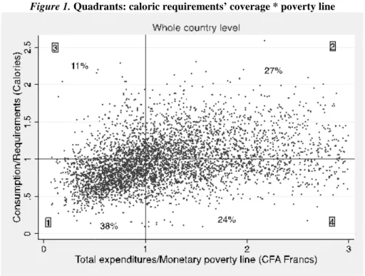
Figure 1is divided into four quadrants on the basis of calories consumed and total expenditure for each household. Calories consumed are presented as proportions of the minimumsufficiency (the horizontal line). Household expenditures are presented as proportions of the poverty line (the vertical line) Quadrant (1) contains households below the poverty line whichare caloriedeficient; quadrant (2) contains households above the poverty line whichare calorie sufficient; quadrant (3) contains households which, although below the poverty line, are also calorie sufficient; and quadrant (4) contains house which are above the poverty line but are calorie deficient.

The “expected” cases (quadrants 1 and 2) represented 65% of the overall population — 67% and 61% in rural and urban areas respectively. The “unexpected” cases (3 and 4) represented 35% of the population — 33% of the rural population and 39% of the urban population.

Figure 1. Quad

4.2 Characteristics related to outputs

The econometric estimate sug quadrants, particularly in quad described in Tables 2and 3. Tab analyses were made in urban a different between these two env the four modalities correspondin McFadden’s pseudo-R2 prese adjustment (Green 2000). Thi variables (it is found in most ap and 0.37 in rural and urban are high.

The hypothesis of the independ dependent variable modalities statistics provided by Hausman the endogeneity of explanatory varia cost of calories), though it was not fo problem is less troublesome. collinearity between some varia the different variables (Table A3

adrants: caloric requirements’ coverage * poverty lin

Source: Authors' estimates.

to different combinations of monetary poverty and fo

suggests ways to characterize the households found adrants 3 and 4. The explanatory variables in the regr

able A4 in the Annex shows the results of this analysis

n and rural areas, as the consumption characteristics a nvironments. There are thus two multinomial logistic re ding to the four quadrants in Figure 1.

sented below in Table A4 allows measuring the q his indicator has a limited value in models with d applications between 0.2 and 0.6: Gujarati, 2004). It is areas in our study, indicating that the quality of our mo

ndence of irrelevant alternatives is valid when the omis s has no effect on the estimated parameters (Green o an tests5 in our case allow us to validate this hypothesis. of explanatory variables arise for some variables in our model ( , though it was not formally tested. However, as our goal is only descri

troublesome. Finally, given the large number of explanatory var riables is high. Correlation tests, however, showed a w A3 shows the matrix of correlation).6

quality of model discrete dependent t is respectively 0.31 model adjustment is

ission of one of the

op. cit.) The Chi2

is. It is likely that in our model (e.g. the average our goal is only descriptive, this variables, the risk of a weak link between

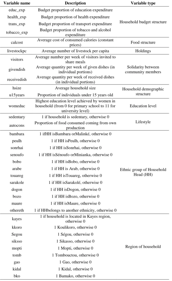
Table 2. Description of variables

Variable name Description Variable type

educ_exp Budget proportion of education expenditure

Household budget structure health_exp Budget proportion of health expenditure

trans_exp Budget proportion of transport expenditure tobacco_exp Budget proportion of tobacco and alcohol

expenditure

calcost Average cost of consumed calories (constant

prices) Food structure

livestockpc Average number of livestock per capita Holdings visitors Average number per week of visitors invited to

share meals

Solidarity between community members givendish Average quantity per week of given dishes (in

individual portions)

receivedish Average quantity per week of received dishes (in individual portions)

hsize Average household size _{Household demographic} structure u15years Proportion of individuals under 15 years old

womeduc

Highest education level achieved by women in household (from 0 for primary school to 11 for

university level)

Education level sedentary 1 if household is sedentary, otherwise 0

Lifestyle autocons Proportion of food consumed coming from own

production

bambara 1 ifHH isBambara orMalinké, otherwise 0

Ethnic group of Household Head (HH) peulh 1 if HH isPeulh, otherwise 0

sonrhai 1 if HH isSonrhai, otherwise 0 senoufo 1 if HH isSénoufo orMinianka, otherwise 0

bobo 1 if HH isBobo, otherwise 0 arabe 1 if HH is Arab, otherwise 0 touareg 1 if HH isTouareg, otherwise 0 sarakole 1 if HH isSarakolé, otherwise 0 dogon 1 if HH isDogon, otherwise 0

bozo 1 if HH isBozo, otherwise 0 maure 1 if HH isMaure, otherwise 0

othereth 1 if HHbelongs to another ethnicity, otherwise 0 kayes 1 if household is located in Kayes region,

otherwise 0

Region of household kkoro 1 Koulikoro, otherwise 0

Segou 1 Ségou, otherwise 0 siksso 1 Sikasso, otherwise 0 mopti 1 Mopti, otherwise 0

tomb 1 Tombouctou, otherwise 0

gao 1 Gao, otherwise 0

kidal 1 Kidal, otherwise 0

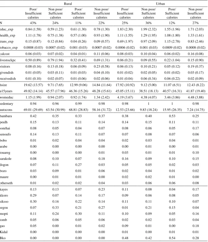
Table 3. Descriptive statistics of variables Rural Urban Poor/ Insufficient calories Non poor/ Sufficient calories Poor/ Sufficient calories Non poor/ Insufficient calories Poor/ Insufficient calories Non poor/ Sufficient calories Poor/ Sufficient calories Non poor/ Insufficient calories N 43% 24% 11% 22% 25% 36% 12% 27% educ_exp 0.84 (1.58) 0.59 (1.23) 0.61 (1.30) 0.78 (1.30) 1.83 (2.30) 1.99 (2.32) 1.55 (1.96) 1.71 (2.03) health_exp 1.11 (1.78) 0.75 (1.38) 0.57 (1.00) 0.93 (1.90) 1.11 (1.55) 1.29 (1.95) 1.08 (1.80) 1.33 (1.61) trans_exp 0.15 (0.87) 0.12 (0.84) 0.04 (0.26) 0.09 (0.57) 0.69 (1.97) 0.97 (2.09) 1.15 (2.78) 0.83 (2.46) tobacco_exp 0.0008 (0.03) 0.0007 (0.02) 0.001 (0.03) 0.0007 (0.02) 0.0006 (0.02) 0.001 (0.03) 0.0009 (0.02) 0.0008 (0.02) calcost 0.06 (0.03) 0.07 (0.02) 0.04 (0.01) 0.11 (0.06) 0.08 (0.03) 0.10 (0.04) 0.06 (0.02) 0.16 (0.08) livestockpc 0.50 (0.89) 0.79 (1.94) 0.32 (0.41) 0.69 (1.31) 0.06 (0.21) 0.09 (0.55) 0.22 (1.04) 0.15 (0.90) visitors 0.08 (0.16) 0.13 (0.18) 0.06 (0.09) 0.23 (0.58) 0.06 (0.13) 0.10 (0.21) 0.05 (0.12) 0.19 (0.37) givendish 0.01 (0.05) 0.03 (0.11) 0.01 (0.03) 0.04 (0.10) 0.01 (0.02) 0.02 (0.05) 0.01 (0.02) 0.03 (0.17) receivedish 0.01 (0.10) 0.02 (0.07) 0.01 (0.06) 0.02 (0.06) 0.01 (0.04) 0.06 (0.34) 0.06 (0.22) 0.02 (0.09) hsize 19.62 (13.57) 9.71 (7.65) 12.99 (9.06) 14.84 (11.64) 17.92 (10.92) 9.12 (5.00) 11.07 (6.51) 12.43 (8.22) u15years 49.82 (14.14) 45.57 (17.96) 46.36 (15.26) 48.28 (15.61) 45.05 (15.11) 38.51 (18.13) 40.57 (16.31) 41.87 (19.40) womeduc 1.15 (1.99) 0.94 (2.07) 0.92 (1.74) 1.34 (2.42) 4.19 (3.67) 4.38 (4.07) 3.46 (3.86) 4.48 (3.88) sedentary 0.94 0.96 0.99 0.98 0.98 1 1 0.98 autocons 69.01 (29.69) 63.54 (30.99) 68.81 (28.83) 58.16 (31.72) 12.53 (23.66) 9.83 (18.24) 15.95 (26.35) 7.24 (14.75) bambara 0.42 0.35 0.33 0.37 0.38 0.40 0.53 0.25 peulh 0.15 0.13 0.11 0.14 0.14 0.15 0.11 0.11 sonrhai 0.08 0.05 0.04 0.07 0.08 0.06 0.05 0.17 senoufo 0.14 0.13 0.11 0.07 0.07 0.08 0.07 0.06 bobo 0.01 0.02 0.04 0.04 0.02 0.03 0.04 0.01 arabe 0.00 0.00 0.00 0.00 0.00 0.01 0.00 0.01 touareg 0.00 0.00 0.00 0.01 0.03 0.01 0.01 0.10 sarakole 0.08 0.10 0.07 0.18 0.16 0.09 0.10 0.15 dogon 0.07 0.11 0.27 0.03 0.05 0.05 0.02 0.03 bozo 0.03 0.09 0.01 0.06 0.02 0.04 0.01 0.02 maure 0.00 0.01 0.01 0.00 0.02 0.02 0.01 0.00 otherseth 0.01 0.02 0.02 0.04 0.03 0.06 0.06 0.08 kayes 0.13 0.13 0.07 0.23 0.11 0.08 0.04 0.17 kkoro 0.29 0.07 0.14 0.17 0.09 0.06 0.08 0.05 siksso 0.30 0.16 0.22 0.14 0.11 0.11 0.10 0.07 segou 0.07 0.33 0.21 0.27 0.01 0.21 0.15 0.04 mopti 0.11 0.24 0.30 0.11 0.10 0.09 0.05 0.16 tomb 0.05 0.06 0.05 0.06 0.02 0.02 0.03 0.04 gao 0.05 0.00 0.01 0.02 0.09 0.01 0.00 0.18 Kidal 0.00 0.00 0.00 0.00 0.01 0.00 0.01 0.01 Bko 0.00 0.00 0.00 0.00 0.48 0.42 0.54 0.28

Note: Figures in parentheses represent standard deviations

The distribution of households across the quadrants in rural and in urban areas was different, especially for the “expected” cases (quadrants 1 and 2). The proportion of poor households with insufficient caloric intake was higher in rural areas than in urban areas (43% versus 25%). On the other hand, the proportion of non-poor with sufficient caloric intake was higher in urban areas than in rural areas (36% versus 24%).

Among the variables studied, the cost of calories and the household size were those that most often explained the position of households across the four quadrants(Table A4). In rural areas, the number of visitors sharing households’ meals and residing in the Koulikoro region werealso important

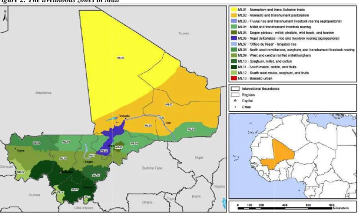
determinants, whatever the quadrant considered. In urban areas, the proportion of children in the household and residing in the Segou, Sikasso, and Gao regions were most often the determinant variables (The Box 2 below presents the main characteristics of the different regions of Mali).

Box 2: Characteristics of the different regions of Mali

Mali is a large landlocked country of West Africa. With a total area of 1.2 millions km2, the majority of the population is involved in agriculturally-based activities. The Northern regions (Tombouctou,

Gao and Kidal) are the most arid with less than 250 millimeters of rainfall per year. These zones are

structurally deficient in terms of food production. The main activities are nomadic and transhumant pastoralism. Mopti is located in the South of Tombouctou and receives up to 600 millimeters of rainfall per year. The main activities are agriculture (dry cereals and rice in the Niger Delta) and agro-pastoralism. Kayes, Koulikoro and Segouare located in the South-West of Mopti. The activities in these regions vary from livestock rearing in the more arid Northern bound to dry cereals production and more diversified agricultural productions in the Southern bound (maize, cotton and fruits). The “Office du Niger” in Segou is the zone where the main irrigation installations for rice production are located. The Northwest of the region of Kayes is known as the zone where the people receive many remittances. Finally, the region of Sikasso at the extreme South of Mali is the most fertile and is often called the attic of Mali. The main products of this region are maize, cotton and fruits.

Before focusing on the paradoxical cases (quadrants 3 and 4), the characteristics of households in the two “expected” cases (quadrants 1 and 2) are presented.

Being non-poor with sufficient caloric intake was associated withhigher cost of calories consumed andlower household size in both rural and urban areas, but these associations were stronger in urban areas than in rural areas.Moreover, in rural areas, being non-poor with sufficient calories was associated withhigher numbers of livestock per capita and higher numbers of visitors sharing the households’ meals.

Being poor with insufficient caloric intake was associated, in both areas, with higher household size (effect of higher household size stronger in rural areas).In rural areas only, being poor with insufficient calorieswasassociated with the consumption of cheaper calories, greater expenditure on tobacco and alcohol, fewer visitors sharing households’ meals,more numerous dishes received and a lower share of own production in the calories consumed.In urban areas only, a higher proportion of children under 15 years old in the householdhad a positive (but weak)effect on the probability of being poor with insufficient calories. In these areas, this probability was also linked to a lower level of women’s education. This finding tracked well with the negative relation between child malnutrition and women’s education shown by previous works such as Smith and Haddad (2002).

Ethnicity is a significant determinant of the above “expected cases” only in rural areas. Belonging to the Sarakole ethnic group in comparison to belonging to the Bambara/Malinké group (the most populous)was strongly and positively associated with the probability of being non-poor with sufficient calories and negatively associated with being poor with insufficient calories.

Some regions were also significantly associated with these probabilities in both areas. Living in the rural areas of Kayes and Koulikoro,when compared to living in the rural areasofMopti (the region randomly selected as the reference), was strongly and positively associatedwith the probability of being poor with insufficient calories and negatively associated with being non-poor with sufficient calories.Living in the urban areas of Segou and Sikasso,when compared to living in Bamako (the biggest urban centre), was strongly and positively associated with the probability of being non-poor with sufficient calories and negatively associated with being poor with insufficient calories. On the contrary, living in the urban areas of Gao,when compared to living in Bamako, was strongly and negatively associated with the probability of being non-poor with sufficient calories, whereas it was positively associated with being poor with insufficient calories.

Quadrants 3 and 4 are now analysedin depth because they areof particular interest to understand why it is sometimes difficult to estimate food insecurity using monetary indicators.

In rural areas, this probability was strongly associated withthelower cost of calories consumed by the household7 andfewer visitors who shared the household’s meals. This probability was also associated with lower household size and a higher share of consumption that came from self-production, but theselinkswere weaker.Moreover, poor households with sufficient calories belonged more to the Sarakoleand Dogonethnic groups rather than the Bambara/Malinke ethnic group, and lived more in the Mopti region rather than the Kayes, Koulikoro, and Sikasso regions.

In urban areas, the probability of being poor with sufficient calories was strongly associated withthelower cost of calories consumed and greater number of livestock owned by the household. This probability was also associated with a lowerproportion of children under 15 years old in the household and a higher proportion of consumption that came from own production, but these links were weaker. Finally, this probability was strongly associated with living in Bamako as opposed to living in Kayes, Segou, Sikasso,orGao.

• Probability of being non-poor with insufficient caloric intake (quadrant 4)

In rural areas, this probability was strongly associated with greater health care expenditure, higher cost of calories consumed, a greater number of visitors sharing meals, and fewer meals received from other households. Moreover, this probability was associated with greater household size, but the link was relatively weak. The non-poor with insufficient calories in rural areas were ofPeulh or Boboethnicity rather than Bambara/Malinke, and lived in the Koulikoro or Segou regions.

In urban areas, being non-poor with insufficient caloric intakewas also strongly associated with the higher cost of calories consumed by the household,agreater number of visitors sharing meals and living in Mopti rather than Bamako There were also weaker associations between this probability and higher transportation expenditure, greater household size, and a greater number of children under 15 years old in the household.

5 Discussion

The results concerning the strong relation between the cost of calories and the probability of being in one quadrant or another mainly reflects two behaviours:

(1) On average, the non-poor consumed more expensive calories than the poor; this is because of the diversification of their diet,which is less centred on staple foods such as local cereals(See Table 1); (2) Thehouseholds that consumed“paradoxically” were those thattended to consume either the least expensive calories (poor with sufficient calories) or the most expensive calories (rich with insufficient calories). This was true in both rural and urban areas.

In rural areas, it is difficult to say whether these findings reflect the households’ preferences to consume cheaper products or an availability constraint: in some remote villages, in the absence of exchange through localmarkets, diets will be limited to items that can be produced in the region. Agro-climatic conditions determine in this case the components of the food basket. Because cereals are the cheapest source of calories and most commonly grown products, this explains the significant relationshipfound between higher self-production and being poor with sufficient calories.

At the urban level, as different foods are available in the market, the findingswere more linked to preferences, at least for the atypical households. The rate of self-consumption was much lower in the cities (results not shown), and thus people could “choose” with fewer constraints and express various preferences.8

The poor consume cheaper calories in general. But, the table of descriptive statistics shows that the poor with sufficient calories consume even cheaper calories than the poor with insufficient calories.

8_{Actually, farming in Mali mainly relies on extensive agricultural systems with very few modern}

inputs. Even if it were possible for farmers to diversify their crops, it would be difficult to do so because of the bad roads and difficulties of accessing inputs. Moreover, as in many other countries, the agricultural policies of the last decades have not encouraged diversification since they have focused on cotton/maize systems and mono-cropping rice. As a result of their isolation (both for accessing inputs and selling outputs), unevenly distributed rainfall, and highly risky natural and economic environment (very low prices of most commodities and production highly unstable) most farmers adopt risk avoidance strategies to insure minimum productionof staple cereals in order to be able to feed their household.

We keep with Sen’s (1992) findings that the differences ofgoals and the variation in the ability to use endowments help to explain differences in behaviour. We also keep withthose of Deaton (1997), for whom the existence ofnon-poor people with an unsatisfactory diet or poor people with an adequate dietare related to the fact that not all householdsspend a sufficient proportion of their revenue on food in terms of nutritional requirements.

Even poor people can have a relatively satisfactory diet (in the sense of their caloric requirementi) if they spend a larger proportion of their budget on food and if they mostly eat low-cost foods (see Table A1).From a case study in several developing countries, Banerjee and Duflo (2007) showed that the poor often spent large sums of money on tobacco, alcohol, or varioustraditional ceremonies. As this expenditure is not “top priority,” they concluded that the poor actually have many choices for managing their budget that would enable them to significantly improve the quality of their food consumption, but they make different choices. These different empiricalstudiesschallenge the hierarchy of requirementsestablished by Maslow. Many people prefer to meet social or private requirements, also regarded as “secondary,” before completely covering their theoretical nutritional requirements. This implies that good nutrition does not necessarily result from improvements in income alone. Nutrition education may be as important for achieving good nutrition.

Moreover, the increased cost of health carein urban areas and of transport in rural areas increases the probability of calorie deficiency despite adequate total expenditure.

The significant effect of the number of guests at mealtime in rural areas means that,in some cases,lesser social costs promote the ability to meet caloric requirements despite limited financial resources, and in others the inability to cover requirements despite a priori sufficient resources.

The significant effect of household size on caloric requirements or lack thereof on the poor and non-poor confirms the negative relationship between the level of caloricintake and the household size found in other studies (Rogers and Lowdermilk 1991; Subramanian and Deaton op. cit.; Abdulai and Aubert 2004a).

Our results are mainly based on the comparison of different types of householdsdefined using a particular crossing of monetary poverty and caloric requirements indicators.The main weakness of the method is the attribution of the same characteristics to different households regardless of their proximity or their distance from the monetary poverty line or from the caloric intake threshold. This does not, however, question the validity of the results for a large portion of the population.

We used the most recent, large, and complete household surveyavailable in Mali, which allowed the simultaneous assessment of both household food consumption, using the weights of the different foods consumed at home and monetary poverty using detailed expenditure data.To our knowledge there is no other survey available in the Sahel that has these characteristics. There are, of course, other more recent surveys called “EnquêteLégèreIntegréeAuprès des Ménages” (ELIM) carried out in 2003, 2006 and 2010. Although these surveys include food consumption information, the method of collection of the data is far less precise because they are based on the recall of quantities and frequencies of different items consumed.

By using data from the 2001 household survey, our purpose was not to give a recent account of food insecurity in Mali but to draw attention to the paradox that poor households below the poverty line may consume sufficient calories while those above the poverty line may consume insufficient calories.Our hypothesis is that the factors explaining thisparadox are more structural than transient, as may be the food insecurity situation.

Determination of the intra-household distribution of calories is beyond the scope of the present study but should be the subject of further research.. Further research is also required to compare poverty indicatorswith more qualitative food consumption indicators, such as nutrient deficiencies as a household may consume many calories but have a very poor diet in terms of essential nutrients.

6 Conclusions

By assigning households to quadrants according to whether or not their caloric requirementsare metand according to their position in relation to the poverty line, we have estimated that 11% of households meet their caloricrequirements although they are poor, and 24% do not meet them even though they are above the poverty line.Thediscrepancy between these two indicators is not intrinsically surprising because the determinants of poverty and food insecurity are not necessarily the same. Yet, for most households, the monetary poverty indicator, most frequently available through surveys of households, adequately reflects satisfaction of caloric requirements’ coverage.

We have shown that non-poor households do not cover their caloric requirements due to eating habits thatare characterized by consumingespecially expensive caloriesand because of certain binding expenditures (health care and transport). In contrast, poor households can meet their requirements when theyconsume inexpensive calories, but this is likely to be at the expense of the overall quality of their diet. These findings challenge a vision which is centred on the need to meet their caloric requirements as the primary goal of the poorest households.

This researchsupports the idea that monetary poverty could be a fairly good indicator of food insecurity, but it raises awareness on precautions to make while measuring food insecurity soleythrough monetary indicators.

Above all, it encourages more frequent use of household surveys in monitoring food security. Acost-effective and precision-conscious way toproceed would consist of completing monetary indicatorswith other available information. These could bespecific food habits, degree of solidarity between households,vulnerability due to health problems or large household size. Moreover, these surveys offer opportunities to analyse further, many other issues for better monitoring of food insecurity and improved food security policies, such as access to inputs in rural areas (land, credit, seeds), access to markets, existence and quality of roads, influence of pricing, also cultural and religious factors.

A deficit in caloricintake is only one aspect of household food insecurity. The results presentedin this studythus encourage further research to describe and analyse the complex relationships between the different dimensions of food insecurity and poverty at the household level.

Acknowledgements

The authors warmly thank:

- Fellow nutritionistsfromUMR NUTRIPASS of IRD for their assistance with consumption data processing, especially Sabrina Eymard-Duvernay, EdwigeLandais

- Fellow statisticians in Mali, especially Ms.AssaGakouDoumbia andBalla Keita from the National Institute of Statistics and SirikiCoulibalyfrom Afristat for their advice for the data recovery; - The two journal reviewers for their detailed comments on earlier versions of this text.

References

Abdulai A. &Aubert D. (2004a). Nonparametric and parametric analysis of calorie consumption in Tanzania.Food Policy, 29(2), p. 113-129.

Abdulai A. &Aubert D. (2004b). A cross-section analysis of household demand for food and nutrients in Tanzania.Agricultural Economics, vol. 31 n°1, p. 67- 79.

Banerjee A. V. &Duflo E. (2007). The economic lives of the poor. The journal of economic

perspectives, 21(1), p. 141.

Bartus T. (2005). Estimation of marginal effects using margeff.Stata Journal, 5(3), p. 309-329. Baulch B. &Masset E. (2003). Do monetary and nonmonetary indicators tell the same story about

chronic poverty? A study of Vietnam in the 1990s.World Development, 31(3), p. 441-453. Behrman J. R. &Deolalikar A. B. (1987). Will Developing Country Nutrition Improve with

Income? A Case Study for Rural South India.The Journal of Political Economy, 95(3), p. 492. Behrman J. R. & Wolfe B. L. (1984). More Evidence on Nutrition Demand: Income Seems

Overrated and Women's Schooling Underemphasized. Journal of DevelopmentEconomics,

14(1-2), p. 105-128.

Bocoum I. (2011). Sécurité alimentaire et pauvreté. Analyse économique des déterminants de la consommation des ménages. Application au Mali. Thèse de doctorat d'Economie, Université Montpellier 1, Montpellier. 245 pages plus annexes.

Bouis H. E. & Haddad L. J. (1992). Are estimates of calorie-income elasticities too high?: A recalibration of the plausible range. J DevEcon, (39), p. 333-364.

Cahuzac E. & Bontemps C. (2008). Stata par la pratique: statistiques, graphiques et éléments de programmation. Stata Press Publ.

Chamberlain G. (1982). Multivariate regression models for panel data. Journal of Econometrics,

18(1), p. 5-46.

Darmon N., Bocquier A., Vieux F. &Caillavet F. (2010).L'insécurité alimentaire pour raisons financières en France. Lettre de l'ONPES (4).

Deaton A. &Drèze J. (2009). Food and Nutrition in india: Facts and interpretations. Economic and

political weekly, 44(7).

Deaton A.S. (1997). The Analysis of Household Surveys: A Microeconometric Approach to Development Policy. Johns Hopkins Univ Pr.

DNSI (2004). Enquête malienne sur l'évaluation de la pauvreté (EMEP) 2001. Principaux résultats. Dop C., Pereira C., Mistura L., Martinez C.& Cardoso E.(2012). Using Household Consumption

and Expenditures Survey (HCES) data to assess dietary intake in relation to the nutrition transition: A case study from Cape Verde. Food & Nutrition Bulletin 33 (Supplement 2): 221S-7S.

Eozenou P., Madani D. &Swinkels R. (2013). Poverty, Malnutrition and Vulnerability in Mali. Policy ResearchWorkingPaper 6561. The World Bank.

FAO, WFP & IFAD (2012). The State of Food Insecurity in the World 2012. Economicgrowthisnecessary but not sufficient to acceleratereduction of hunger and malnutrition. Rome, FAO.

Fiedler J.L. (2012). Towards overcoming the food consumption information gap: Strengthening household consumption and expenditures surveys for food and nutrition policymaking. Global

Food Security (2012), doi: http://dx.doi.org/10.1016/j.gfs.2012.09.002

Green W.H. (2000).Econometric Analysis. Fourth Edition. Prentice-Hall International. 1004 p. Gujarati D. N. (2004). Econométrie. Traduction de la 4ième edition américaine. De Boeck. 1009 p. Haddad L. (2009). Lifting the Curse: Overcoming Persistent Undernutrition in India. IDS Bulletin,

40(4), p. 1-8.

Headey D.D.(2013). The Impact of the Global Food Crisis on Self-Assessed Food Security.The

World Bank Economic Review, 27(1), p. 1-27.

Murphy S., Ruel M.&Carriquiry A.(2012). Should Household Consumption and Expenditures Surveys (HCES) be used for nutritional assessment and planning? Food & Nutrition Bulletin

33 (Supplement 2): 235S-41S.

Nordeide M. B. (1997). Table de composition d'aliments du Mali. Institut de Nutrition. Oslo : Université d’Oslo.

Ohri-Vachaspati P., Rogers B.L., Kennedy E. & Goldberg J. P. (1998). The effects of data collection methods on calorie–expenditure elasticity estimates: a study from the Dominican Republic. Food Policy, 23(3-4), p. 295-304.

Pradhan M., Suryahadi A., Sumarto S. & Pritchett L. (2001). Eating Like Which" Joneses"?An Iterative Solution to the Choice of a Poverty Line" Reference Group".Review of Income and

Wealth, 47(4), p. 473-488.

Ravallion M. (1998). Poverty Lines in Theory and Practice.World Bank Publications.

Rogers B. L. &Lowdermilk M. (1991).Price policy and food consumption in urban Mali.Food

Policy, 16(6), p. 461-473.

Samaké A., Bélières J-F.,Corniaux C., Dembele N., Kelly V., Marzin J, Sanogo O. &Staatz J. (2008). Changements structurels des économes rurales dans la mondialisation. Programme RuralStruc Mali-Phase II: MSU IER Cirad.

http://siteresources.worldbank.org/AFRICAEXT/Resources/RURALSTRUC-MALI_Phase2.pdf

Sen A. K. (1992). Repenser l'inégalité. Traduction française de InequalityReexamined. Paris, Éditions du Seuil.

Smith L.C. & Haddad L. (2002). How Potent is Economic Growth in Reducing Undernutrition? What Are the Pathways of Impact? New Cross-Country Evidence.Economic Development and

Cultural Change, 51(1), p. 55-76.

Smith L.C. &Subandoro A.(2007). Measuring Food Security Using Household Expenditure Surveys, Food Security in Practice. Washington DC: International Food and Policy Research Institute.

Svedberg P.(1999). 841 Million Undernourished?World Development, 27(12), p. 2081-98. doi: 10.1016/s0305-750x(99)00102-3

Svedberg, P.(2000). Poverty and undernutrition: Theory, measurement, and policy. Oxford University Press, USA.

Svedberg P.(2002). Undernutrition Overestimated. Economic Development and Cultural Change,

51(1), p. 5-36.

Strauss J. & Thomas D. (1995). Human resources: Empirical modeling of household and family decisions. Handbook of development economics, 3(1), p. 1883-2023.

Subramanian S. & Deaton A. (1996). The Demand for Food and Calories.Journal of Political

Economy, 104(1), p. 133.

Swindale A. &Ohri-Vachaspati P. (2005).Measuring household food consumption: a technical guide. 2005 ed.

Figure 2: The livelihoods zones in Ma

Source: FEWS-NET

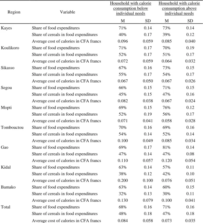
Table A1. Main characteristics of household food consumption by region in relation to the level of calorie consumption

Region Variable

Household with calorie consumption below

individual needs

Household with calorie consumption above

individual needs

M SD M SD

Kayes Share of food expenditures 71% 0.14 73% 0.14

Share of cereals in food expenditures 40% 0.17 39% 0.12 Average cost of calories in CFA francs 0.096 0.059 0.085 0.040

Koulikoro Share of food expenditures 71% 0.17 70% 0.19

Share of cereals in food expenditures 52% 0.17 51% 0.17 Average cost of calories in CFA francs 0.072 0.059 0.064 0.032

Sikasso Share of food expenditures 67% 0.16 73% 0.15

Share of cereals in food expenditures 55% 0.17 54% 0.17 Average cost of calories in CFA francs 0.067 0.050 0.067 0.026

Segou Share of food expenditures 66% 0.15 71% 0.15

Share of cereals in food expenditures 45% 0.15 47% 0.16 Average cost of calories in CFA francs 0.082 0.038 0.067 0.024

Mopti Share of food expenditures 69% 0.15 76% 0.12

Share of cereals in food expenditures 52% 0.19 56% 0.17 Average cost of calories in CFA francs 0.071 0.041 0.058 0.028

Tombouctou Share of food expenditures 70% 0.16 69% 0.16

Share of cereals in food expenditures 54% 0.14 52% 0.14 Average cost of calories in CFA francs 0.100 0.049 0.085 0.034

Gao Share of food expenditures 69% 0.17 81% 0.14

Share of cereals in food expenditures 47% 0.14 47% 0.08 Average cost of calories in CFA francs 0.110 0.057 0.120 0.054

Kidal Share of food expenditures 63% 0.14 57% 0.11

Share of cereals in food expenditures 38% 0.12 42% 0.10 Average cost of calories in CFA francs 0.200 0.100 0.076 0.051

Bamako Share of food expenditures 63% 0.14 60% 0.15

Share of cereals in food expenditures 32% 0.13 30% 0.11 Average cost of calories in CFA francs 0.130 0.079 0.100 0.041

Total Share of food expenditures 68% 0.16 71% 0.16

Share of cereals in food expenditures 48% 0.18 47% 0.18 Average cost of calories in CFA francs 0.084 0.058 0.073 0.035

M: Mean; SD: Standard Deviation. Source: Authors' estimates.

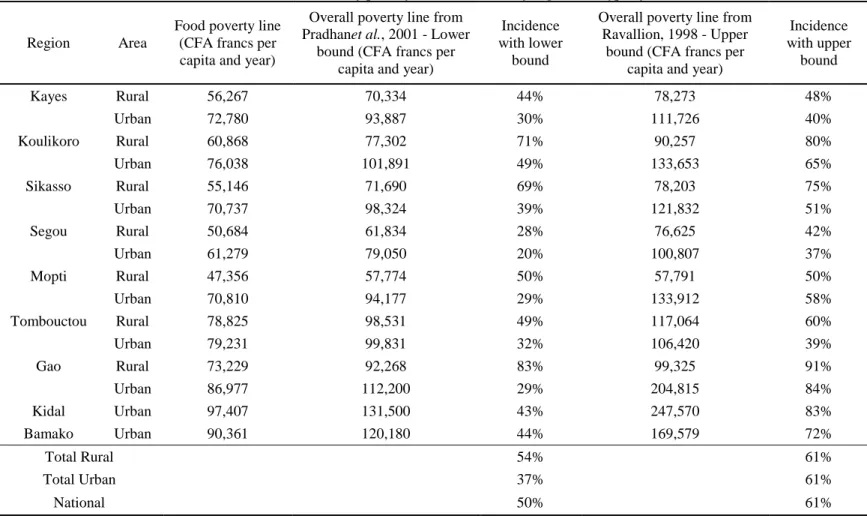
Table A2. Monetary poverty lines calculated by region and type of area

Region Area

Food poverty line (CFA francs per capita and year)

Overall poverty line from Pradhanet al., 2001 - Lower

bound (CFA francs per capita and year)

Incidence with lower bound

Overall poverty line from Ravallion, 1998 - Upper

bound (CFA francs per capita and year)

Incidence with upper bound Kayes Rural 56,267 70,334 44% 78,273 48% Urban 72,780 93,887 30% 111,726 40% Koulikoro Rural 60,868 77,302 71% 90,257 80% Urban 76,038 101,891 49% 133,653 65% Sikasso Rural 55,146 71,690 69% 78,203 75% Urban 70,737 98,324 39% 121,832 51% Segou Rural 50,684 61,834 28% 76,625 42% Urban 61,279 79,050 20% 100,807 37% Mopti Rural 47,356 57,774 50% 57,791 50% Urban 70,810 94,177 29% 133,912 58% Tombouctou Rural 78,825 98,531 49% 117,064 60% Urban 79,231 99,831 32% 106,420 39% Gao Rural 73,229 92,268 83% 99,325 91% Urban 86,977 112,200 29% 204,815 84% Kidal Urban 97,407 131,500 43% 247,570 83% Bamako Urban 90,361 120,180 44% 169,579 72% Total Rural

educ_exp health_exp trans_exp tobacco_exp calcost livestockpc visitors givendish receivedish hsize u15years womeduc sedentary educ_exp 1.0000 health_exp 0.0989 1.0000 trans_exp 0.0668 0.0861 1.0000 tobacco_exp -0.0668 -0.0164 -0.0219 1.0000 Calcost 0.0800 0.0188 0.0704 -0.1106 1.0000 Livestockpc -0.0674 0.0122 -0.0368 0.0146 -0.0225 1.0000 Visitors -0.0350 0.0329 -0.0328 -0.0087 0.2978 0.0308 1.0000 Givendish -0.0203 0.0159 -0.0121 -0.0387 0.2482 0.0131 0.3361 1.0000 Receivedish -0.0150 0.0100 0.0009 0.0679 0.0525 0.0208 0.0983 0.0760 1.0000 Hsize 0.0523 0.0422 -0.0109 0.0088 -0.2044 -0.0098 -0.1742 -0.1150 -0.1021 1.0000 u15years 0.0219 -0.0195 -0.0716 -0.0499 -0.2085 -0.0561 -0.1126 -0.0586 -0.0660 0.1863 1.0000 Womeduc 0.3672 0.0799 0.1337 -0.1451 0.2416 -0.1258 -0.0490 -0.0055 -0.0262 0.0717 -0.1250 1.0000 Sedentary -0.0074 0.0175 0.0237 -0.0210 0.0487 -0.0226 0.0058 -0.0008 0.0084 -0.0075 -0.0091 0.0485 1.0000 Autocons -0.2115 -0.0250 -0.1177 0.1413 -0.3511 0.1265 -0.0493 -0.0639 -0.0490 0.2180 0.1322 -0.3863 -0.0150 Bambara -0.0022 0.0228 0.0177 0.0790 -0.0825 -0.0157 -0.0676 -0.0636 -0.0353 0.0550 0.0099 0.0266 -0.0078 Peulh -0.0553 -0.0213 -0.0022 -0.0275 0.0066 0.0615 0.0085 -0.0017 -0.0115 -0.0526 -0.0292 -0.0399 -0.0313 Sonrhai -0.0185 -0.0044 -0.0197 -0.1072 0.1180 -0.0294 0.1063 0.1784 0.0525 -0.1158 -0.0072 0.0053 0.0235 Senoufo 0.1101 0.0776 0.0120 -0.0368 -0.0409 0.0262 -0.0174 -0.0197 0.0086 -0.0150 0.0046 0.0438 0.0078 Bobo 0.0172 -0.0276 0.0003 -0.0033 -0.0410 0.0314 -0.0081 0.0026 -0.0021 -0.0053 0.0102 0.0084 0.0027 Arabe 0.0008 0.0014 -0.0014 0.0030 0.0666 -0.0200 0.0134 -0.0040 0.0042 -0.0344 0.0025 0.0085 0.0106 Touareg -0.0320 -0.0265 -0.0265 -0.0024 0.1314 -0.0302 0.0561 0.0093 0.0309 -0.0771 -0.0107 -0.0356 -0.0066 Sarakole 0.0291 -0.0211 -0.0113 0.0267 0.0329 -0.0073 -0.0050 -0.0216 -0.0106 0.1347 0.0251 -0.0187 0.0047 Dogon -0.0213 -0.0409 0.0025 0.0451 -0.0783 -0.0241 -0.0178 -0.0213 -0.0286 0.0163 0.0104 -0.0215 0.0277 Bozo -0.0295 -0.0101 0.0049 -0.0017 -0.0166 0.0127 0.0085 -0.0157 0.0093 0.0001 0.0075 -0.0314 -0.0269 Maure -0.0169 0.0166 -0.0137 -0.0306 0.0008 -0.0037 0.0354 -0.0062 0.0052 -0.0214 -0.0184 -0.0176 0.0178 Othereth 0.0070 -0.0034 0.0099 -0.0101 0.0375 -0.0292 -0.0159 -0.0037 0.0352 0.0073 -0.0123 0.0423 0.0048

autocons bambara peulh sonrhai senoufo bobo arabe touareg sarakole dogon bozo maure othereth autocons 1.0000 bambara 0.1423 1.0000 peulh 0.0083 -0.3517 1.0000 sonrhai -0.1762 -0.2609 -0.1308 1.0000 senoufo 0.1003 -0.2405 -0.1205 -0.0894 1.0000 bobo -0.0070 -0.1209 -0.0606 -0.0449 -0.0414 1.0000 arabe -0.0765 -0.0585 -0.0293 -0.0217 -0.0200 -0.0101 1.0000 touareg -0.1550 -0.1215 -0.0609 -0.0452 -0.0416 -0.0209 -0.0101 1.0000 sarakole -0.0451 -0.2770 -0.1388 -0.1030 -0.0949 -0.0477 -0.0231 -0.0479 1.0000 dogon 0.0778 -0.1874 -0.0939 -0.0697 -0.0642 -0.0323 -0.0156 -0.0324 -0.0740 1.0000 bozo -0.0244 -0.1359 -0.0681 -0.0505 -0.0466 -0.0234 -0.0113 -0.0235 -0.0536 -0.0363 1.0000 maure -0.0231 -0.0981 -0.0492 -0.0365 -0.0336 -0.0169 -0.0082 -0.0170 -0.0387 -0.0262 -0.0190 1.0000 othereth -0.0891 -0.1754 -0.0879 -0.0652 -0.0601 -0.0302 -0.0146 -0.0304 -0.0692 -0.0468 -0.0340 -0.0245 1.0000