Land Development and Pigouvian Taxes:
The Case of Peatland
Renan
u.
Goetz
In this paper the determination of an optimal Pigouvian tax for a competitive firm when a negative production externality is present concurrent with the development of land for production purposes is analyzed within a dynamic framework. Conditions are established for a convex social net return function where a Pigouvian tax is not required or where the imposition of a Pigouvian tax leads to the decision not to develop the land at all. In the case of a concave social net return function the Pigouvian tax is either a linear or a nonlinear tax on the private net returns.
Key words: dynamic optimization, land development, negative production externalities, Pigouvian taxes.
Pigouvian taxes can be considered as a first-best. environmental policy to achieve the so-cially desired ends if it is possible to mea-sure the costs and benefits associated with the externality (Cropper and Oates). Apart
from the question of whether or not
Pigouvian taxes can be applied in reality, other issues related to Pigouvian taxes have been raised. Spulber analyzed the long-run efficiency properties of Pigouvian taxes and established an entry-exit condition for a long-run equilibrium that must be satisfied for an efficient outcome. Lee and Barnett proposed a second-best Pigouvian tax in light of imperfect competition in the pres-ence of negative externalities. Baumol and Bradford showed that detrimental externali-ties tend to induce nonconvexity of the social production possibility set even if individual producers face a convex production possibil-ity set. As a result, there may exist a multi-plicity of local maxima, leaving the
determi-The author is a research associate in the Department of Agricul-tural Economics, Swiss Federal Institute of Technology, ZUrich, Switzerland and currently a visiting professor in the Department of Economics, University of Girona, Spain.
This paper was written while the author was visiting the Depart-ment of Agricultural and Resource Economics, University of Cali-fornia at Berkeley. An earlier version of this paper was presented at the VIII Congress of the European Association of Agricultural Economists, Edinburgh, 3-7 September 1996. Financial support from the Swiss National Science Foundation is gratefully acknowl-edged. The author thanks Michael Hanemann and two anonymous reviewers for their comments and helpful suggestions.
nation of the global social maximum open. A similar result was obtained by Starrett where the failure of the second-order conditions arise from the nonconcavity of the function representing the firm's production function as it is affected by a negative externality.
In this paper the development' of peatland for agricultural production where empirical evi-dence shows that the traditional assumption of strong concavity of the producer's net return function might not hold is characterized. In pre-vious papers, the assumption of concavity is violated because producers of different goods are negatively affected by each other. By con-trast, in this paper the nonconcavity of the net return function results from the opportunity of the producer to switch to production of more valuable goods through developing more of the essential and limiting factor, land quality. For the case of a convex social net return function, the optimal private and social outcome may be identically given by an upper boundary solu-tion, and no Pigouvian tax is required. How-ever, a Pigouvian tax may lead to the farmer's decision not to develop the land at all.
Ifthe social and the private net return func-tions are concave, a linear Pigouvian tax on the private net return function induces the farmer to achieve the optimal social outcome. However, if the private net return function is convex, a nonlinear Pigouvian tax on the farmer's net re-turns is required to generate the optimal social outcome.
Amer. J.Agr. Econ. 79 (February 1997): 227-234 Copyright 1997 American Agricultural Economics Association
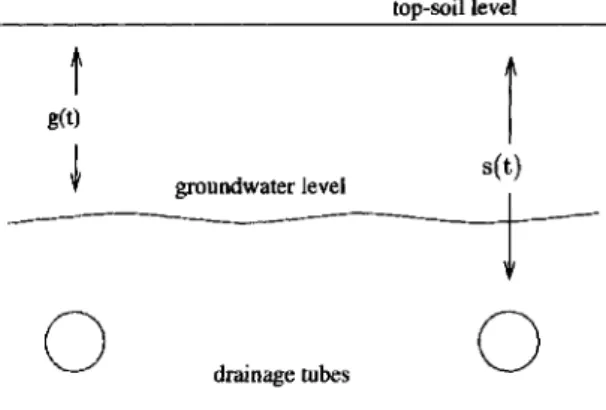
Figure1. Cross section of drained peatland
IIn Finland and Sweden, for instance, 33.5% and 15.6% of the entire land respectively is covered with peat (Pfadenhauer et al.).
drained up to 75 em, the farmer optimally can grow corn and various small grains, while draining the peatland to a depth of up to 100 em enables the farmer optimally to grow veg-etables (Poiree and Ollier, Maslov and Panov). The subsidence of peatland located in central western Europe from these farming practices ranges between 1-4 em per year. The associated net return function 1t(g), is a monotonically in-creasing function ing with 1t(0)
=
O. The lower the groundwater level, chosen by the farmer, the more valuable the crops that can be grown at the expense of high subsidence rates of the soil. Depletion of the peat stock, however, re-duces the future profitability of the land, and thus the farmer faces a trade-off between high immediate net returns for a shorter period of time versus lower net returns for a longer pe-riod of time.As a case study for a particular area, the choice of the optimal intertemporal groundwa-ter level for a net-return-maximizing farmer has been analyzed by Goetz and Zilberman. How-ever, they did not consider the potential pollu-tion of the groundwater and surface water with nitrogen (N) in the form of nitrate as a result of the mineralization of the organic material. In Germany, where nearly the entire fen peatland is utilized for agricultural production (Gottlich and Kuntze), or in states or countries like Min-nesota, Canada, or North Europe where large peatlands can be found, mineralization of the organic material is likely to affect the groundwater or surface water quality.' More-over, peatland often serves as a habitat for en-An Economic Model for the Development of
Peatland
The origin of peatland (organic soil) and its special properties in comparison with mineral soil have been described in detail by Goetz and Zilberman. They also described the key charac-teristics of the agricultural utilization of peatland, so we will be relatively brief with re-spect to these issues.
Under specific climatic and hydrologic con-ditions, plant residue does not completely decompose, which gives rise to the growth and deposit of peat. Peat is characterized by a high content of organic material and nutrients, and thus peatland is particularly interesting for agri-culture. For example, peat contains on average more than 2.5% of nitrogen in the dry matter compared to 0.03%-0.3% for mineral soil (Kuntze, Roeschmann, and Schwerdtfeger). Growing crops on peatland requires developing the land beforehand by installing a drainage system. Inevitably, this will lead to the subsid-ence of the land due to an initial loss of volume and to a nearly constant rate of mineralization of the organic material (Schothorst). Segeberg has shown that the subsidence is directly pro-portional to the groundwater level and can be mathematically expressed as
(1) s = -[f(t)
+
y]g(t)where a dot over a variable denotes the opera-tor dldt and t time. The variable s(t) represents the distance between the topsoil level and the drainage tubes (peat stock) (i.e., the amount of soil developed), j the subsidence of the peatland, f(t) an exponential distribution of time, y>0 the constant mineralization rate, and g(t) the distance between the topsoil level and the groundwater level. For a graphical illustra-tion of the points of reference to measure the variables s(t) and g(t), see figure 1.To simplify notation, the argument t of s,f, g and z,
A,
<1>;, i= 1, 2, 3 (to be introduced later), will be sup-pressed unless it is necessary for an unambigu-ous notation.
Different crops require for their optimal growth particular groundwater levels which can be set by the farmer by means of controlled drainage, either in the form of subirrigation or irrigation. Hence, the groundwater level deter-mines the kind of crops that can be grown. A groundwater level of approximately 50 em is optimal for growing grass. If the peatland is
t
g(t)o
groundwater level drainage tubes top-soil levelr
s(t)o
dangered species of plants (Briemle). There-fore, its value as an environmental asset should be compared with the social benefits from the agricultural utilization of the peatland. Conse-quently, providing a benchmark for the decision as to whether (a) to continue agricultural pro-duction on peatland or to restore its natural state by raising the groundwater level to the top soil level; or (b) to convert intact peatland into pro-ductive agricultural land or to conserve it, should include negative production externalities.
The N-mineralization for peat ranges from 300 to 1,200 kg N per hectare (ha) per em peat loss. Even perennial crops like grassland are only able to assimilate 500 kg/ha of N per year. Although some of the mineralized N is biologi-cally denitrified and lost as gas in the form of NzO (Guthrie and Duxburg), a high share of the mineralized N is expected to leach into the groundwater or run into surface waters. Kuntze measured the N content of the groundwater re-charge per hectare cultivated with agricultural crops. He found that the admissible 11.0 kg N/ ha per 100 mm groundwater recharge for meet-ing N03 regulations for drinking water in the European Community was not satisfied, reach-ing concentration levels up to six times above the standard.
Equation (1) shows that the groundwater level is proportional to the subsidence of the soil, and consequently as well to the release of nitrogen, denoted by z. Moreover, the release of nitrogen is monotonically increasing with g.As such, there exists a functional relationship ~z=
g, ~ > 0 and equation (1) and the net return function can be written as
II
(P)
~,~x
J
e-ol<p(z)dto
subject to
s =
-if
+ y)~Z, s(O)So,Z
E Z "{Z : Z
= 0; a "Z
s
b;Z
s
*}
where ()> 0 presents the social discount rate, and tI denotes the end of the planning horizon.
The maximum life span of the installed drain-age system is given by T and places an upper bound on t); therefore t) E [0,
n.
As stated above, peatland can be utilized for agricultural production when g is between 50 and 100 em, which corresponds to the values a and b for the control variable z. Moreover, as a physical ne-cessity, g must always be smaller than s, which yields the constraint S - ~z ~ O. The currentvalue Hamiltonian is therefore given by H
=
1t(~z) - e(z) - A(f+y)~z, where Adenotes the costate variable. Taking account of the con-straints on the control variable z, we obtain the following Lagrangian: L
=
H+<p)(z -
a) +<Pz(b- z)+
<pls -
~z)where <Pi' i= 1, 2, 3, represents the Lagrange multipliers. A solution for prob-lem (P) has to satisfy the following necessary conditions which are stated in accordance with propositions 2.5 and 6.1 of Feichtinger and Hartl:(2) s=
-if
+y)~z, 1t(~z).(5) s
=
-if
+y)~z, s(O)=
Sowhere the subscript with respect to a variable denotes the corresponding partial derivative. Moreover, the optimal values of the control variable
z
and the Lagrange multipliers have to satisfy the Kuhn-Tucker conditions: L$i ~ 0, <Pi~ 0 and <PiL$i =0, for i= 1, 2, 3. The constraint
qualification will be satisfied due to the linear-ity of the restrictions in
z
(Takayama). The transversality conditions are given byIn the presence of a negative production exter-nality given by the pollution of the groundwater and surface water, the costs and benefits of abating nitrate need to be considered. Hence, to ensure efficiency we assumethat a social plan-ner exists, and thus the social net return func-tion is given by <p(z) = 1t(~z) - [k(z) + d(z)],
where k(z) denotes the costs and d(z) the ben-efits of abating the negative production exter-nality. In line with the literature, it is proposed that k+d is convex (see, for example, Baumol and Oates and Pearce). To simplify the notation we setk(z) +d(z) = e(z)and refer to e as social costs.
Now, we are able to state the optimal control problem for the social planner:
(6)
(
t ) >
TJ
for
Note that q>(a)
=
<p(a) and q>(b)=
<p(b); other-wise <p > q>. Next, we will replace q> in problem (P) with <p a'ld denote this problem by(P). The linearity of (P) in z suggests the definition of a switching function, a,given by(7) A(t\) ~0 S(t\) - ~a ~0 A(t\)[S(t\) - ~a]
=
0where complementary slackness applies to the last expression, and the superscript * indicates the evaluation along the optimal path. The eco-nomic interpretation of the necessary condi-tions is deferred to a later section where we analyze the optimal trajectories of sand z to-gether with the different qualitative properties of the social net return function.
(8) <p = [n(~a) - c( a)]b - [n(~b) - c( b)]a
b-a
+
{n(~b)
- c(b) -[n(~a)
- c(a)]}z.b-a
Plgouvlan Taxes
Based on Swiss data, Goetz and Zilberman showed thatneg) is strictly convex and that it is optimal for the individual farmer to drain the land to the upper limit and to deplete the soil as fast as possible over the entire time horizon. In this paper we will not restrict ourselves to this particular example. More importantly, taking account of the social costs of the negative pro-duction externality in the form of groundwater or surface water pollution may alter the qualita-ti ve properqualita-ties of the problem (P). Even if
n(~z) is strictly convex in z. the function q>(z) can either be convex or concave in z, depending on whether n(~z) orc(z)has the stronger curva-ture. To analyze the implications of these quali-tative properties on the trajectories of s* and
z*,
we will first discuss the case where q> is convex, and thereafter where q> is concave.The Social Net Return Function is Convex The qualitative properties of the optimal trajecto-ries can be obtained by the following proposition.
PROPOSITION 1. If the social net return func-tion, given in problem (P), is strictly convex in
z,
the optimal trajectory ofz
is a boundaryso-lution.'
Proof. The idea is to reduce the convex prob-lem to that of a linear one by the construction of a linear function <p whose graph lies above that of q>. This function is given by
2For the case wherecpis convex, the function can be partitioned
such thatcpis strictly convex or linear on intervals of z. On these intervals, cpcan be analyzed in the same way as described in proposition1.
(9) a(t)
=
Hz
n(~b) - c(b) - [n(~a) - c(a)]
= b _ a - A(f+I')~.
As is known flom the theory of optimal control, maximizing H requires the following choices:
(10)
z
=
[z : •
:~:~: ~].
a , aCt) < 0
Ifa singular path,
a
=0, occurs for some posi-tive interval of time, then the optimal trajectory of z can also lie in the interior of Z. Let us as-sume that a singular path exists. Hence, forsom~positive interval of time,
cr =
-'A
if
+I')~- Af~=0 has to hold, which yields
'A
j
=
-A
f
+
I'Utilizing equation (4) for an interior value of Z results in
(11)
j
=
-'O(f+1').The general solution of this differential equa-tion isfit)
=
c\e-& - 1', where c\ is a constant. However, substitutingf(t) in equation (2) shows that 1', the constant of mineralization, cancels out, changing the qualitative properties of ex-pression (2). Thus, we can conclude that c\eSt-I' is not an admissible solution and no singular path for any z in the interior of Z exists. Hence z* takes on a boundary value.
So far, we obtained",qualitative properties of z* for the problem (P). However, since q> of
problem (P) is strictly convex in z. the subsid-ence of peatland is linear in z, and the switch-ing function orr) associated with problem (P) does not vanish over a time interval of positive length, theorem 3.3 of Feichtinger and Hartl can be employed. This theorem suggests that the replacement of cp by cP in problem (P) yields the same optimal values for s", z', A*, where z* is given by 0,
a,
b, orslJ3.
More pre-cisely,Land Development and Pigouvian Taxes 231 vate net return function. We know further that1t is monotonically increasing, and thus proposi-tion 1 suggests that the optimal private trajec-tory of z is chosen from the upper boundary of the set Z.3 However, the convexity of cp does
not determine the sign of cp', which in turn leaves the determination of the optimal value of z open. Let us first consider the case wherecp'>0
(12) z' =
argmax{max[
H(O.A.
t),
tu».
A.
t),
H(b,A,
t),
H(i-.A.
t)]}
3This result can be obtained even though proposition I requires strict convexity. As indicated in footnote 2 an appropriate partition of the private net return function enables us to apply proposition I for the different segments of the partition. In the case where the segment is strictly convex, proposition I can be applied directly.If
the segment is linear, then a boundary solution also can be estab-lished by the fact that the switching function does not vanish over a positive interval of time.
forcp>0, and the socially and privately optimal trajectories are identically given by an upper boundary value of Z. In this case, there is no need to correct the market outcome because it is also optimal from the social point of view. However,
if cp' =1t' - c' < 0 for cp>0, say fort >
t,
thenthe privately and socially optimal outcomes are distinct, and the market outcome needs to be corrected such that the farmer chooses a. For the case cp<0, it would be socially optimal not to drain the land at all. Thus, a tax
would induce the optimal social outcome where z; refers to the optimal private outcome. Hence, at point
t
the farmer would either switch to z=
a or to z=
O. However, regardless of the optimal social outcome beyond timet,
the farmer may choose not to develop the land at all since the investment in the drainage sys-tem may no longer be profitable when 't isin-corporated in a cost benefit analysis.
For the calculation of the tax 't the function
c(z) needs to be known over the interval [a, b]. When this function is not available, an upper bound to social costs can be obtained provided that information exists supporting the convexity where the variables s and
A
of the right-handside of equation (12) have to be evaluated for the given boundary value of z.
In other words, in the case of a strictly con-vex social net return function, with respect to agricultural production, it may be optimal to drain the land as deeply as possible or as shal-low as possible, or not at all.Ift, <Tand none of the Hamiltonians evaluated at H(a,
A,
t,),H(b,
A,
t,), H[(s/~),A,
t,] is zero, then the transversality condition (6) requires that we choose z(t,)=
0 at the terminal point of time. Thus, the peatland will be utilized for agricul-tural production as long asH(a,A,
t), H(b,A,
t) and H[(s/~)A,
t] are strictly positive. Ifthis condition fails to be satisfied over time, the uti-lization of the peatland for agricultural pur-poses would be terminated and the groundwater level would be raised to the topsoil level. Simi-larly, if t, = T and H(a,A,
t,), H(b,A,
t,), andH[(s/~)
A,
td are strictly negative, thenz(t,)=
0 also has to be chosen to satisfy equation (6). However, ifH(a,A,
t), H(b,A,
t), andH[(s/~)A,
t] ~0, for all t, then z*(t,) ~O. For this case, it may be optimal to leave the minimum layer of peat or even more in the ground.
Social versus private outcome for the convex
case. Next, we will analyze the conditions for
an optimal social outcome, which is distinct from an optimal private outcome, and requires a regulator to correct the market outcome. Note that the case of a convex social net return func-tion implies that the private net return funcfunc-tion, 1t, is also convex. Otherwise, the social net re-turn function as a sum of two concave func-tions, 1t(~z) and -c(z), would also be concave. Moreover, the convexity of cp also requires that cp" ~ c", The case of a linear social cost func-tion, for example, would give rise to a convex social net return function, given a convex
pri-(13) { 0 . 't(t) = ' c(z;); t
~ ~}
t > t232 February 1997
of the function over the interval [a, b], and the points c(a) and c(b) are known. A linearization of c(z),denoted by v(z), is given by
(14) v(z)
=
c(a)b - c(b)a +(C(b) - c(a)]zb - a b - a
negligence of the social costs, the optimal pri-vate strategy reaches the boundary before the optimal social strategy."
To analyze the possibilities for a regulator to correct the market outcome, we introduce an ad valorem tax t. Thus, the necessary condition for the solution of the farmer's problem yields where v(z) >c(z)for z E (a, b), and v(a)
=
c(a)and v(b)
=
c(b). Replacing c(z) with v(z) in problem (P) and solving for the optimal trajec-tory ofz
yields a boundary solution. Ifthe con-sideration of the negative production external-ity has no effect on the optimal private out-come, no Pigouvian tax needs to be imposed. Hence, the upper bound of the social cost serves as a benchmark to decide whether or not the market outcome needs to be corrected at all.The Social Net Return Function is Concave In contrast to the previous section we look now at optimal solutions lying in the interior or at the boundary of Z. The transversality condition
(7) for the case of an interior solution shows that
ACtI)
= 0, given s(tl ) - ~a >O. Next,solv-ing equation (4) yields A(t)= Aje-°r,whereA j~0 is determined by the condition A(tj )
=
O. How-ever, this implies thatACt)
=
0, contradicting the dynamic properties of problem (P). Hence, we can conclude that an interior solution over the entire time interval [to, tl ] is not possiblebe-cause the requirement s(t j) = ~a = ~z*(tj) can-not be satisfied. At least at the terminal point in time,
z
takes on a boundary value.(17) (1 - "t)1t'(~z)~- 'A(f+y)~- <l>3~ = 0
A(t
+ y) + <1>3~ "t(z) = 1
-1t'(~z)
where we consider the example of a boundary solution for set) = ~z. Ifthe regulator sets the tax equal to "t(
z;),
thenz;,
the solution to the necessary condition of the social problem given in equation (16), also solves the necessary con-dition of the private problem, given in equation (17). In other words, the individual farmer chooses the groundwater level which is identi-cal with the socially optimal groundwater level. In this way, the optimal private and social strat-egies will reach the boundary at the same time, and no tax is required for the time thereafter.Ifn, however, is convex, any linear tax "t on the private net return will not alter the curva-ture of 1t, and the private outcome is always given by a boundary solution. To obtain a pri-vate strategy which lies in the interior of Z and is identical with the social strategy, a nonlinear tax on private net returns is required. We pro-pose three different tax schemes, where the first one, in the form of a step function, is the limit-ing case of the second one. Consider the fol-lowing tax:
4The proof can be obtained from the author upon request. For any upper deviation from the socially opti-mal water pollution level the tax is prohibitive, but it is equal to zero for any lower deviation from the optimal social strategy. While this tax is easy to administer, it is most likely not politi-cally feasible since it basipoliti-cally places a cap on the farmer's net returns. A tax which is continu-ously increasing but starting out low for small upper deviations may be politically easier to in-troduce. For the derivation of this tax, math-ematically expressed as "t[1t(~z)], consider first Social versus private outcome for the
con-cave case. In order to compare the social out-come with the private outout-come we need to de-fine some qualitative properties of 1t. Let us as-sume for now that 1t, besides<p,is concave. For an interior solution, the optimal private strategy
z;
differs from that of the optimal social strategyz;
as can be seen from the necessary conditions for an interior solution of the private and social problem, given respectively by(15) 1t'(~z)~= A(f+y)~
(16) 1t'(~z)~- c'(z)
=
A(f+y)~.Moreover, we know that every optimal solution that starts as an interior solution will tum into a boundary solution after some time. Because of
(18)
(
0 . 1t(~z)::; 1t(~z;)).
"t[1t(~z)]= '
the necessary condition for an interior solution of the private problem given by
where equation (19) was utilized. One candi-date for the tax, satisfying equations (19) and (20), is given by
Equation (19) has to hold at z=
z;.
The second-order condition, which has to hold for any z>z;,
implies (19) {I - 't'[1t(~z)J}1t'(~z)~ - A(f + I'O~=
0 A(f + y) ~ 't'[1t(~z)]= 1 - . 1t'(~z) SummaryInitial or repeated land development for agri-cultural production results in groundwater and surface water pollution in the case of peatland. As shown in the literature, the farmer's net re-turn function may not be concave since farmers switch to the production of more valuable crops as more soil becomes available. Thus, taking account of the additional costs from the water pollution may result in a convex or concave so-cial net return function. In the case where the social net return function is convex, the pri-vately and socially optimal outcomes may be identical and no market correction is required. However, if the two outcomes are distinct, a Pigouvian tax is proposed which leads to a less intensive use of the land or to the decision not to develop the land at all. Even if the optimal
~"[
n(J3z)1
> [n"(J3z)1
AU13+
y)
[1t'( Z)]3 (20) (21) { 0 3 2 ;1t(~z)::; 1t(~z;
)}.'t[1t(~z)]
=
-l[1t(~z)F
- A(f +y)~z
+_z- - _z_.
1t(A Z) >2 3(Z;)2 2(z;) , .... 1t(~z;)
The tax scheme in equation (21) induces the net-return-maximizing farmer to choose
z;.
The first two taxes, as proposed in equations (18) and (21), are not directly related to the monetary damage from the water pollution. Thus, they can be seen as a method to imple-ment a certain standard. The third proposed possibility for the regulator to correct the mar-ket outcome is to employ the social costs c(z) as a tax scheme. Because this tax scheme re-flects the monetary damages accurately, it seems to be superior to the first two tax schemes. However, the implementation of this tax would require information about z, which may not be easily observable. Instead of z it would be easier to observe the farmer's net re-turns. Hence, we consider the invertible func-tiony = 1t(~z).The tax can now be expressed as a function of the farmer's net returns and is given by
social outcome suggests the extensive use of the land, the farmer may decide not to use the land at all because investing in the drainage system is no longer profitable due to the impo-sition of a Pigouvian tax.
The case where the private as well as the so-cial net return function are concave results in a linear Pigouvian tax on the private net return function. However, if the social net return func-tion is concave while the private net return function is convex, a linear Pigouvian tax on the private net return function does not exist which corrects the market outcome such that the socially optimal outcome, given by an inte-rior solution, is chosen by the farmer. To ac-complish this objective, three different tax schemes are proposed, where the tax is a non-linear function on the private net returns.
[ 1t-1
(y)]
(22) 't[1t(~z)] = c -~- .
[Received June 1995;
final revision received January 1997.]
Faced with this tax, the net-return-maximizing farmer chooses
z;
that is identical to that given by the solution to the necessary conditions for an interior solution for the private and social problems.References
Barnett, A. "The Pigouvian Tax Rule Under Mo-nopoly." Amer. Econ. Rev. 70(December 1980): 1037-41.
234 February 1997
Baumol, W., and D. Bradford. "Detrimental Exter-nalities and Non-convexity of the Production Set." Economica 39(May 1972):160-76. Baumol, W., and Oates, W. The Theory of
Environ-mental Policy, 2nd ed. Cambridge: Cambridge
University Press, 1988.
Briemle, G. "N atiirliche Bewaldungstendenz und Mindestpflege von Moorbiotopen." Moor- und
Torfkunde, 3rd ed. K. Gottlich, ed., chap. 5.5.
Stuttgart: E. Schweizerbart'sche, 1990.
Cropper, M., and W. Oates. "Environmental Eco-nomics: A Survey." J. Econ. Lit. 30(June
1992):675-740.
Feichtinger, G., and R. Hartl. Optimale Kontrolle
Okonomischer Prozesse. Berlin: Walter de
Gruyter, 1986.
Goetz, R,and D. Zilberman. "Mining the Soil-Ag-ricultural Production Systems on Peatland."
Environ. and Resour. Econ. 6(September
1995):119-38.
Gottlich, K., and H. Kuntze. "Natiirliche Bewaldungstendenz und Mindestpflege von Moorbiotopen." Moor- und Torfkunde, 3rd ed., K. Gottlieb, ed., chap. 5.1. Stuttgart: E. Schweizerbart' sche, 1990.
Guthrie,T., and J. Duxburg. "Nitrogen Mineralization and Denitrification in Organic Soils." Soil Sci.
Amer.J.42(NovemberlDecember 1978):908-12. Kuntze, H. The Risks of Water Pollution by
Agricul-tural Utilization of Peatlands and Practical De-fense. Proceedings of the 7th International Peat
Congress, International Peat Society, Dublin, Ireland: 18-23 June 1984, pp. 246-67.
Kuntze, H., G. Roeschmann, and G. Schwerdtfeger.
Bodenkunde, 4th ed. Stuttgart: Eugen Ulmer,
1988
Lee, D. "Efficiency of Pollution Taxation and Mar-ket Structure."J. Environ. Econ. and Manage.
2(September 1975):69-72.
Maslov, B., and E. Panov. Peat Soils: Improvement
and Agricultural Use in the USSR. Proceedings
of the 6th International Peat Congress, Interna-tional Peat Society, Duluth MN, 17-23 August 1980, pp. 421-25.
Pearce, D. Environmental Economics. London: Longman, 1976.
Pfadenhauer, J., H. Schneekloth, S. Schneider, and
R Schneider. "Stellung der Moore im Raum."
Moor- und Torfkunde, 3rd ed. K. Gottlich, ed., chap. 2. Stuttgart: E. Schweizerbart'sche, 1990. Poiree, M., and C. Ollier. Assainissement Agricole.
Paris: Eyrolles, 1978.
Schothorst, C."Subsidence of Low Moor Peat Soils in the Western Netherlands." Geoderma. 17(April 1977):265-91.
Segeberg, H. "Moorsackungen durch Grundwasserab-senkungen und deren Vorausberechnung mit Hilfe empirischer Formeln." Zeitschrift piir
Kulturtechnik und Flurbereinigung. l(January/
February 1960):144-61.
Spulber, D. "Effluent Regulation and Long-run Optimality." J. Environ. Econ. and Manage.
12(June 1985):103-16.
Starrett, D. "Fundamental Nonconvexities in the Theory of Externalities." J. Econ. Theory.
4(April 1972): 180-92.
Takayama, A. Mathematical Economics, 2nd ed. Cambridge: Cambridge University Press, 1985.