Development of designer-relevant Lattice-Boltzmann Wind Field Model for urban canyons and their neighborhoods

Development of Designer-Relevant Lattice-Boltzmann

Wind Field Model for Urban Canyons and Their Neighborhoods

By

Tianyi Chen

B.Eng. Environment Engineering Tsinghua University, China, 2014

SUBMITTED TO THE DEPARTMENT OF MECHANICAL ENGINEERING IN PARTIAL FULFILLMENT OF THE REQUIREMENTS FOR THE DEGREE OF

MASTER OF SCIENCE IN MECHANICAL ENGINEERING AT THE

MASSACHUSETTS INSTITUTE OF TECHNOLOGY JUNE 2016

0 2016 Massachusetts Institute of Technology. All rights reserved.

Signature of Author:

Signature redacted

Department of Mechanical Engineering

Certified by:

Signature redacted

Certified by:

Accepted by:

3ignature redaci

0 _{Leslie K. Norford} Professor of Building Technology

Led

e"11- -Steven B. Leeb

Professor of Mechanical Engineering and Electrical Engineering

Signature redacted

Department

MASSACHUSETTS INSTITUTE OF TECHNOLOGY

JUN 022016

LIBRARIES

Rohan C. Abeyaratne Professor of Mechanical Engineering Chairman, Committee for Graduate Theses

Development of Designer-Relevant Lattice-Boltzmann

Wind Field Model for Urban Canyons and Their Neighborhoods

By

Tianyi Chen

Submitted to the Department of Mechanical Engineering on May 6, 2016 in Partial Fulfillment of the Requirements for the Degree of

Master of Science in Mechanical Engineering

ABSTRACT

Wind field analysis is one of the most important components for designers to achieve a thermally-comfortable and energy-efficient building design. Designers need a fast and relatively

accurate wind field model to get integrated into the design workflow, but current platforms to work on are either costly and time-consuming conventional Computational Fluid Dynamics (CFD) tools or over-simplified data correlation factors, which makes the workflow undesirable for designers' use.

In this thesis, a novel Lattice-Boltzmann Wind Field Model (LBWFM) is developed and integrated in a designer-relevant Rhino-based environment. Lattice-Boltzmann Method (LBM) is introduced as the solver due to its open-source and parallelism natures, and coded in C# language for three-dimensional urban airflows. Results of the model are validated with experimental measurements as well as conventional CFD tools for both wind velocity and pressure fields. To further enhance the computational efficiency, proper settings of inlet wind profile and optimal modeling domain size are investigated for the LBWFM. And the relative wind pressure coefficient calculated out of the model is then applied in the analysis of wind-driven natural ventilation potential with the indicator of air exchange flow rate. Finally the limitation of the model is stated aiid future work is discussed on the modifications of buoyancy effect and potential extension is addressed in the application of LBWFM.

Thesis Supervisor: Leslie K. Norford Title: Professor of Building Technology

Reader in Department: Steven B. Leeb

Acknowledgment

I am very grateful to my advisor, Prof. Leslie K. Norford, for his mentoring, guidance and support on both my academics and research. Two years before, I was new to the area of building technology when I first came to MIT. With his passion and patience on the introduction to the scope of research interests, I became more and more informed and motivated to my research topic of development of a designer-relevant wind field model. I admire his kindness to share his new thoughts and ideas with me, and appreciate his encouragement when I got stuck and felt frustrated. I have also learned a lot from his rigorous attitude to the research work, especially his comments on every word and sign in the thesis. I really look forward to my continuous work with him in the coming years for my PhD.

I am also thankful to Prof. Steven B. Leeb, my thesis reader from the Department of Mechanical Engineering. He provided his valuable advice in my course selection and helpful comments on my thesis as well.

I would also like to thank the entire faculty and labmates in the Building Technology Program as well as faculty members from the Department of Mechanical Engineering. Special thanks to Prof. Leon Glicksman for his comments on the natural ventilation potential analysis, and to Dr. Timur Dogan for his efforts on the connections of the model with Grasshopper components. Many thanks for Prof. Christoph Reinhart and Prof. Leslie K. Norford to apply the Lattice-Boltzmann wind field model into real urban site modeling in their class contents and test the robustness and applicability of the model through class assignments. Also thanks for Prof. Rex Britter and Dr. Chao Yuan who gave me insightful instructions on the fundamentals and simulations of urban airflow modeling. Additional thanks to Kathleen Ross and Leslie Regan, whose commitment and spirits made the everyday work convenient and enjoyable.

Finally, I would like to thank my parents and grandparents as well as my friends who were always standing behind me, devoting their strong love, support and encouragement to my studies and work in MIT. They inspired me to do my best and provided every care on my life here.

The research has been funded by the MI-MIT (Masdar Institute - Massachusetts Institute of Technology) flagship project, Development of advanced microclimate and urban energy analysis modeling environment and its validation by wide area sensor networks and remote sensing for future adaptation of urban infrastructure.

Contents

1

1.1 Background ... 15

1.2 Wind field modeling for urban canyons and their neighborhoods ... 17

1.2.1 Physical processes happening in urban canyons... 17

1.2.2 Building morphology in urban canyons and their neighborhoods... 19

1.2.3 Typical approaches in wind field modeling field ... 21

1.3 Current designer workflow in building simulation ... 22

1.4 The objective of the research ... 23

2 Principles of Lattice-Boltzm ann M ethod ... 26

2.1 Introduction...26

2.2 Governing equation ... 28

2.3 Boundary conditions...35

2.4 Numerical Stability ... ... 38

2.5 Concluding remarks ... 39

3 Validation of Lattice-Boltzmann method in wind field modeling... 42

3.1 W ind velocity field ... 42

3.1.1 Case description ... 42

3.1.2 Results and Discussions ... 44

3.1.3 Comparisons with wind-tunnel measurements ... 46

3.2 Pressure field ... 50

3.2.1 Case description ... 50

3.2.2 Results and Discussions ... 52

3.2.3 Com parisons with CFD simulation results... 54

4 Derivation of inlet velocity profile and numerical modeling domain ... 57

4.1 Three kinds of wind profile... 57

4.1.1 The logarithmic profile... 57

4.1.2 Modifications on the logarithmic profile and evaluation of aerodynamic properties...60

4.1.3 The exponential profile... 64

4.1.4 The uniform profile ... 67

4.1.5 Sum mary...71

4.2 Momentum transport from the rural area to the urban canyons ... 72

4.2.1 From rural reference location to rural boundary layer ... 72

4.2.2 From rural boundary layer to urban boundary layer...74

4.2.3 From urban boundary layer to urban canopy layer ... 75

4.3 Adjustment distance along the fetch ... 76

4.4 Setup for numerical modeling domain... 78

5 Lattice-Boltzmann wind field model in designer's workflow... 80

5.2 Designer use guide for Lattice-Boltzmann wind field model... 83

5.2.1 Inputs by users ... 83

5.2.2 Outputs for users ... 85

5.3 M odeling interface in Rhino-based environment ... 86

6 Application of Lattice-Boltzmann wind field model in natural ventilation analysis...89

6.1 W ind pressure coefficient... 89

6.2 Indicator of natural ventilation potential - Air exchange flow rate ... 91

6.3 Case Study ... 95

7 Lim itation and Discussion ... 102

7.1 Buoyancy effect on wind patterns in urban canyons...102

7.2 Limitation of Lattice-Boltzmann wind field model ... 103

7.3 Feasible modifications on the model ... 105

8 Conclusions and future work ... 110

List of Figures

Figure 1.1. Generalized cross-section of a typical urban heat island (Oke 2002) ... 15

Figure 1.2. Energy sources and consumption patterns in the US. (Adopted from the Energy Information Administration / Annual Energy Review 2014) ... 16

Figure 1.3. Sketch of thermal and mechanical processes in urban canyon areas. Red arrows refer to possible heat transfer approaches (solid line as short wave radiation and broken line as long wave radiation); and blue cycles refer to turbulence generated in street canyons ... 18

Figure 1.4. Definition of building morphometric parameters (Grimmond and Oke 1999)...19

Figure 1.5. Current designer workflow for wind field analysis ... 23

Figure 1.6. Improved designer workflow for wind field analysis ... 24

Figure 2.1. Schematic of different approaches to transport problems ... 28

Figure 2.2. Schematics of the lattice arrangements in 2D or 3D cases ... 32

Figure 2.3. The two different schemes to implement bounce-back boundary conditions ... 36

Figure 2.4. Bounce-back process in determination of the second-order boundary conditions (Upw ind direction is from north)...37

Figure 2.5. Schematic of periodic boundary conditions implemented by the LBM ... 38

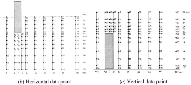
Figure 3.1. Schematic of wind-tunnel experiments and test point locations (Architectural Institute of Japan, 2003) ... 44

Figure 3.2. Vector velocity field in horizontal and vertical sections simulated by LBM ... 45

Figure 3.3. Data correlations for wind velocity between the LBM simulation and wind tunnel experiment at centerline vertical plane (y = 0) 100 mm downstream (at Position 100) ... . . 46

Figure 3.4. The vertical wind velocity profiles from the LBM simulation and wind tunnel experiment. Locations of the vertical lines: 75 mm upstream (Position -75) and 100 mm downstream (Position 100) from the building block ... 47

Figure 3.5. Data correlations for wind velocity between the LBM simulation and wind tunnel experiment at centerline vertical plane (y = 0) ... 48

Figure 3.6. Data correlations for wind velocity between the LBM simulation and wind tunnel

experiment at horizontal plane (z = 12.5 mm, corresponding to human respiratory zone) ... . . 49

Figure 3.7. Schematic of the uniform building community and the numerical modeling domain

with wind coming from left (constructed in Rhino) ... 51

Figure 3.8. Pressure field in horizontal plane simulated by scSTREAM and schematics of test

points ... . . 53

Figure 3.9. Pressure field in horizontal plane simulated by LBM ... 54

Figure 3.10. Data correlations for wind pressure between the LBM simulation and conventional

CFD results at horizontal plane 2 m above the ground level (z = 2 m, corresponding to hum an respiratory zone) ... 55

Figure 4.1. Conceptual representation of the relation between height-normalized values of

zero-plane displacement (zd/ZH) and roughness length (ZO/ZH) and the plan area density (2p, left)

and the frontal area density (F, right). (Grimmond and Oke 1998) ... 61

Figure 4.2. Variation of the attenuation coefficient with array packing density. (Macdonald

2 000) ... 67

Figure 4.3. Sketch of the simplified wind profile (right) approximated with real case (left).

(B ritter 2003) ... 68

Figure 4.4. Comparison of exponential and uniform profile in different building communities

with different frontal area density 2f. (Exp / Uni refers to exponential / uniform profile;

@# refers to the values of h.) ... 70

Figure 4.5. Schematic of the atmospheric boundary layer. (Britter and Hanna 2003) ... 73 Figure 5.1. Lattice-Boltzmann wind field model implemented in designer's workflow ... 81 Figure 5.2. Grasshopper components constructed for LBWFM interface in a Rhino-based

environm ent ... 86

Figure 6.1. Schematic of airflow through an orifice (wind blows from outside to inside of the

building) ... . 92

Figure 6.2. Schematic of airflow through opposite building openings (wind blows from left to

right) ... . . 93

Figure 6.3. Wind pressure contour map in horizontal plane (at the height of respiration zone, z =

Figure 6.4. Comparisons of wind pressure coeffcient in horizontal plane for the three cases ....97

Figure 6.5. Comparisons of wind velocity in horizontal plane for different building heights ....98

Figure 6.6. Comparisons of wind pressure coefficient in horizontal plane for different aspect

List of Tables

Table 4.1. Evaluation of the two aerodynamic properties in three different classes of building

communities (Values extracted from Grimond and Oke 1999) ... 63

Table 4.2. Parameter values in the comparative study cases (including aerodynamic properties

and meteorological measurements) ... 69

Chapter 1

Introduction

1.1 Background

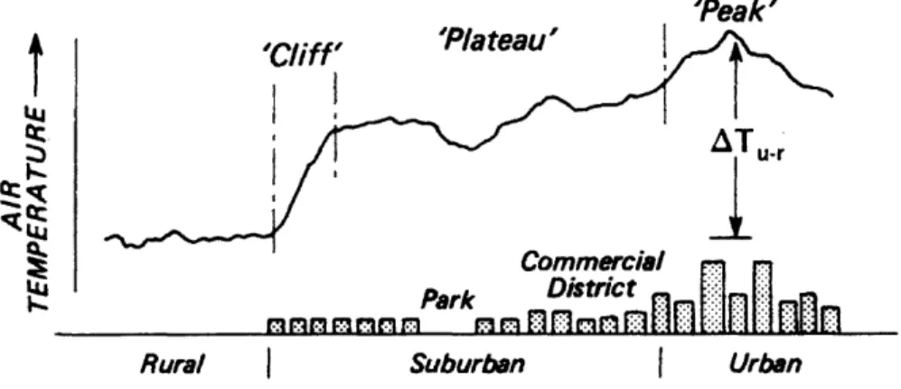
With the fast pace of urbanization, the outdoor air temperature in urban areas is increasing compared to rural areas, a phenomenon known as the Urban Heat Island (UHI) effect. Thermal mass is concentrated in the urban areas where building densities are relatively high, solar and anthropogenic heat is trapped and air temperature goes up. As is shown in Fig 1.1, the outdoor air temperature remains at a low level in the rural areas until at the edge of suburban areas, where buildings become piled up and air temperature climbs up the "cliff." Close to the urban center, ambient temperature arrives at the peak level and the temperature difference between rural and urban areas reaches the maximum.

'Peak'

Cliff, 'Plateau'

Commercial

Park District

Rural I Suburban | Urban

Figure 1.1. Generalized cross-section of a typical urban heat island (Oke 2002).

Meanwhile, most residents live in the urban areas, and urban heating can also have an impact on indoor air temperature and human thermal comfort, which inherently correlate to building energy consumption. Fresh air is needed for the indoor environment, and it inevitably requires a certain amount of air exchanged with outdoor environment. Hot inlet air will mix with the air inside and

thus raise the overall temperature, which imposes higher cooling loads to achieve a comfortable indoor thermal condition, especially in hot seasons. And it results in larger operational energy consumption for the buildings. Fig 1.2 shows the energy flow map for the US in 2014, where building energy consumption (residential and commercial) accounts for over 40% of the total energy sink and heating and cooling loads takes up a large proportion (Ghoniem 2011). Facing the global warming effect largely caused by emissions of energy consumption by-products, CO2,

countries and cities are obligated to manage and reduce the building energy costs, thus achieving energy-efficient building communities.

Pt oleurn E17 I<. AN 019k JIMAY - ' gtn' 61 IN Others Imports St k Chang 0.19

Includes lease condensate. ' Includes 0.16 quadri

2 Natural gas plant liquids. " Total energy consum 3 Conventional hydroelectric power, biomass, geothermal, solar/photovoltaic, and wind. sales, and electrical syt

4 Crude oil and petroleum products. Includes imports into the Strategic Petroleum Reserve, proportion to each secto

5 Natural gas, coal, coal coke, biofuels, and electricity. Energy Losses, at the

6 and unaccounted for. Notes: - Data are presAdustmenss, :ases,

7 Natural gas only; excludes supplemental gaseous fuels. publication. - Totals m Petroleum products, including natural gas plant liquids, and crude oil buned as fuel. Sources: U.S. Energ

. Includes -0.02 quadrillion Btu of coal coke net imports. Tables 1.1, 1.2,1.3, 1.4a II

Ilion Btu of electricity net imports.

ptlion, which is the sum of primary energy consumption, electricity retail

stem energy losses. Losses are allocated to the end-use sectors in r's share of total electricity retail sales. See Note 1, "Electrical Systems mnd of U.S. Energy Information Administration, Monthly Energy Review liminary. -Values are derived from source data prior to rounding for y not equal sum of components due to independent rounding.

y Information Administration, Monthly Energy Review (March 2015), 1.4b, and 2.1.

Figure 1.2. Energy sources and consumption patterns in the US. (Adopted from the Energy Information Administration / Annual Energy Review 2014)

In order to construct a thermally comfortable and energy-efficient building community, we need to have a better understanding of the urban microclimate with characteristics such as wind, temperature, humidity etc. Analysis of the microclimate is mostly focused on urban canyons, the local outdoor areas surrounded by buildings where humans live and work. Urban canyons are

considered as a simplified miniature of many common urban landscapes and act as the connections between the indoor and outdoor environment.

1.2 Wind field modeling for urban canyons and their neighborhoods 1.2.1 Physical processes happening in urban canyons

Urban canyons, as shown in Fig 1.3, are typically comprised of high-rise buildings on the lateral sides and streets in between. In order to well understand the urban microclimate, we need to get an idea of the physical processes occurring in urban canyons.

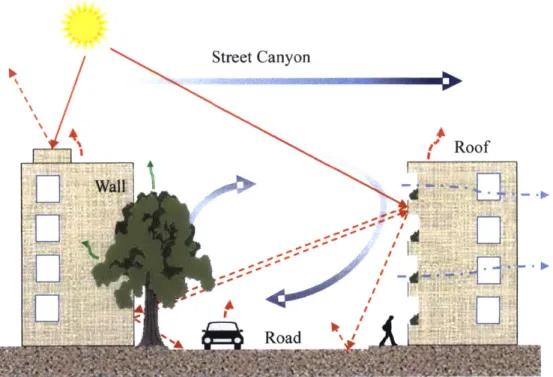
One important aspect is the thermal process originated from the solar radiation. After reflection, scattering and absorption by clouds and other atmospheric constituents, the remainder of the shortwave solar heat flux will irradiate the surfaces that sky can directly see, mostly on the building roofs and the upper part of the walls and sometimes on the road when the building intervals are large. When the radiation contacts the surface, part of it will be absorbed into the building materials, and another gets reflected. Due to the larger density in urban areas, the building fagades are quite close to each other, and the reflection between the neighboring walls will trap a lot of heat in the canyons. At the same time, the large amount of thermal mass will also emit the previously absorbed heat to the canyons and the outer atmosphere in the form of long-wave radiation. Convective heat transfer can happen when there is wind in the region. Conduction takes place along different layers of the building blocks and ground when temperature gradients exist. Human activities and transportation emit anthropogenic heat to the urban canyons, which is also an ineligible contributor to the urban heating. Trees and plants, however, can take in the heat trapped in the canyons and use their evaporation system to reduce the heating effect.

Another important phenomenon is the mechanical process mainly driven by the wind. As is shown in Fig 1.3, at high levels, the wind field is not affected by the massing and retains the same speed and direction from upstream. However, when it gets close to the building height level, the shear layer on the building top deflects the upstream wind and creates circulation and turbulent mixing within the urban canyons. Wind can help facilitate the convective heat transfer

process and flush out the heat concentrated in the canyons as well as pollutants emitted by the human beings. In addition, pressure differences on the opposite sides of the building fa~ades will push the wind across the openings, which will meet the cooling requirement by natural ventilation.

Street Canyon

Roof

Wall

Road

A

Figure 1.3. Sketch of thermal and mechanical processes in urban canyon areas. Red arrows refer

to possible heat transfer approaches (solid line as short wave radiation and broken line as long wave radiation); and blue cycles refer to turbulence generated in street canyons.

To evaluate the microclimate in urban canyon areas, we should take a careful look at the wind fields as they play a significant role in the thermal and mechanical processes happening in the region. The wind field connects the transport of air momentum and heat, and determines the magnitude of convective heat transfer process. It also acts as an important factor in evaluation of outdoor thermal comfort (ASHRAE 2013). Furthermore, the wind field greatly affects the natural ventilation process, since this passive building system depends largely on wind-driven and buoyancy-driven flows. In addition, the wind field mainly determines the pollutant dispersion behavior, which in turn, would influence the indoor energy consumption, i.e. the choice of natural cooling or mechanical cooling systems. In order to guarantee the indoor air quality and

keep healthy, residents will be reluctant to open the windows and let outdoor air circulating across the room to remove the heat if it is highly polluted outside. All in all, studies for wind fields in urban canyons are helpful for predictions of urban microclimate and building energy analysis.

1.2.2 Building morphology in urban canyons and their neighborhoods

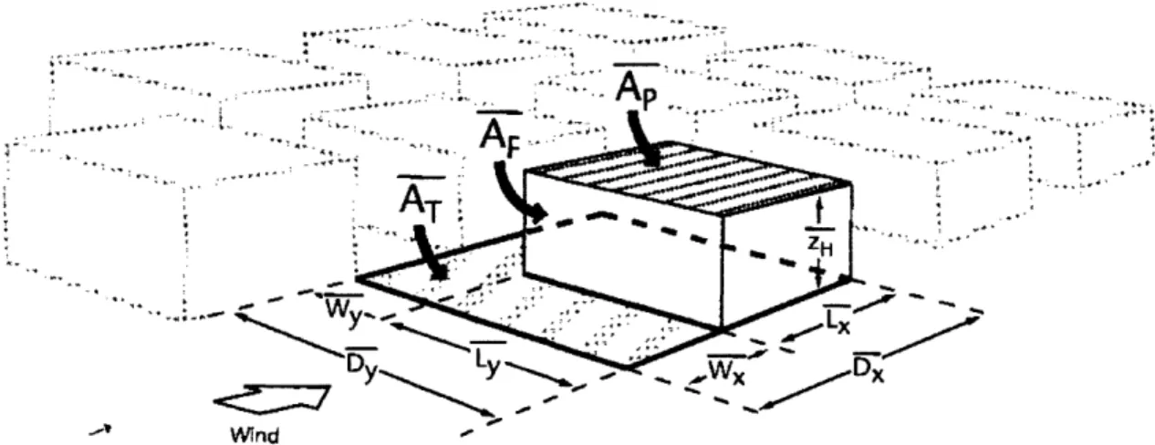
Building morphology determines the characteristics of the urban canyons, and it is one of the most important impact factors for the wind field in urban areas. Parameterization of building morphology contributes to a qualitative description of the massing and its interactions with wind environment. Fig 1.4 gives a sketch of a building community 'as well as the geometric parameters and we can then define the building morphometric parameters based on the geometry marked in the figure. Note that although drawn as building-like, the element is generic, representing all obstacles relevant to airflow. Similarly, the concept is not limited to a grid array. It could include scattered trees, differently shaped houses, and winding streets that are more typical of real cities (Grimmond and Oke 1999).

Ap

D Y Ly .WX Dx

Figure 1.4. Definition of building morphometric parameters (Grimmond and Oke 1999).

The characteristic length of an urban canyon is the area-average building height, which sums up the total volume of the massing in the community and averages over the total horizontal area.

h = YA(QH /Y A (1.1)

Where the overbar of the geometric parameters means that the value is averaged over local roughness and the following expressions will not include them for simplicity. Ap refers to the plan area or projected area of the building in the horizontal plane and ZH refers to the height of the building.

The following three non-dimensional morphological parameters describe the density of the building community in different perspectives. The first parameter, the plan area density p, describes the massing density in the horizontal plane, and it is defined as the ratio of plan area Ap to the total lot area AT of the building community.

XP= AP/AT= L.L,/DDY (1.2)

In contrast, the frontal area density ). describes the massing density in the vertical plane, and it is defined as the ratio of frontal area Af to the total lot area AT of the building community. Note that the frontal plane refers to the projected vertical area orthogonal to upwind direction.

Xf =Af/AT = ZHLy/DxD, (1.3)

Note that both these two density parameters can be extended to the overall average property of the building community if the numerator and denominator are sums of the all the buildings.

The last parameter, aspect ratio /1, describes the density of the urban array, and it is defined as the ratio of building height ZH to the width of the streets w in between two neighboring buildings.

Note that the canyon aspect ratio can be extended to the overall average property of the building community if both numerator and denominator refer to the area-average property of the entire area as similarly defined in Equation (1.1).

1.2.3 Typical approaches in wind field modeling field

There are two prevailing approaches to obtaining a reasonable prediction of wind fields in urban canyons.

One possible method is to use conventional Computational Fluid Dynamics (CFD) tools to calculate dynamic wind flow patterns. These advanced CFD models, based on the continuum hypothesis, solve coupled non-linear Partial Differential Equations (PDEs) with respect to mass, momentum and energy conservation. Detailed turbulence models, e.g. Reynolds-Averaged Navier-Stokes (RANS) equations, Large-Eddy Simulation (LES), etc., are used in the atmospheric turbulence simulation and these models are embedded in many commercial CFD tools, e.g. Fluent, CFX, etc. Although researchers agree on the fact that they can present details on non-uniform facet heat exchange processes and turbulence patterns in canyon areas, the computational costs of these advanced CFD tools are not trivial and needed further consideration in designers' work. Obviously, for instance, designers cannot tolerate waiting a couple of hours in front of computers to see the wind modeling results by a simple shift of building blocks to a certain direction or a small change in building geometries. Besides, these CFD tools are commonly not open source software, and designers also pay a large amount of money for the license of commercial tools, which increases the simulation cost and thus makes CFD analysis hard to apply widely in building design optimization.

The other approach is to use data assimilation methods to correlate wind-field parameters, like the velocity ratio, defined as the ratio of local velocity to a reference velocity, with building geometries, e.g. the planned and the frontal building areas. But the result is very site-specific, and the method requires a large amount of experimental data for the correlation, which increases the overall cost of purchase, installation, operation and maintenance of those measuring tools. What's more, the result is only limited to spatial-average values and takes in little consideration of local turbulence effect in urban canyons. So it is not accurate enough for designers' use in

wind-field modeling, especially at neighborhood scales, where the domain size is relatively small and needs detailed local information of wind field results.

Within a tradeoff of accuracy, computational efficiency and financial costs, the Lattice-Boltzmann Method (LBM) shows its prospective potential by its parallelism and open-source nature (Chen et al. 1998), which are welcome to the workflow of building design. Details of LBM are further explained in Chapter 2.

1.3 Current designer workflow in building simulation

Although wind field simulation by conventional CFD tools is usually expensive and time-consuming, most of the design projects still refer to those results for design optimization because of their wide use and acceptable accuracy. Fig 1.4 shows the current workflow for wind field analysis by conventional CFD tools. It starts from the initial building design from designers, when a pool of CAD-related software is utilized, e.g. Rhino, AutoCAD, etc. To run the wind field simulation, designers must consult building simulation engineers with CAD files exported for the design geometry. But in most cases, the design output contains relatively complex geometries not compatible with CFD software, and engineers must simplify the geometry first. Then discretization is performed for numerical scheme to operate on, with the help of the third commercial mesh-maker software. After setting up the grids, the coupled Navier-Stokes (NS) and energy solver is used and the numerical results are typically routed to a post-possessor to exhibit the wind field map. After that, results are interpreted by engineers and returned to designers for reference. If designers have some further modifications on the design product, another iteration is processed and so on, until the results are satisfactory for the building design.

Looking at the current workflow, we notice that there are many transitions among different commercial software, from the design tool to the simulation solver and from pre-possessors to post-possessors. On the one hand, designers must collaborate a lot with engineers and pay for the simulation results. On the other hand, engineers must master the use of all these commercial CFD tools, and beforehand reconstruct a simplified geometric model for simulation if necessary.

A lot of time and money is expended in the transitions, which acts in opposition to the necessity of wind field analysis.

Software I (RhIno; AutoC AD; ...)

Software 11 (ANSYS. Mesh-maker) software II (Commercial CFD tool) Software IV (ANSYS; Tecplot; ...) Design cad file Pre-possessing (meshing/gridding) Core Function (NS-Energy Solver) Post-possessing (Visualization) Result interpretation

Figure 1.5. Current designer workflow for wind field analysis.

1.4 The objective of the research

The objective of the research is to develop the Lattice-Boltzmann Wind Field Model (LBWFM) to simplify the workflow of the wind field analysis. The most important improvement of

LBWFM compared with conventional CFD tools is that it is entirely compatible with Rhino-based environment for designers, using the visual scripting language integrated with Rhino software, Grasshopper, to connect building design and wind field modeling. The model is open source, and well packaged with designer-relevant inputs and outputs, so designers can directly operate on the modeling platform themselves according to their needs. At the same time, the LBWFM is aimed to achieve fast and relatively accurate results, which makes it possible for designers to get feedback from the wind field in a shorter time. Engineers act as the backup force to manage and modify the LBWFM according to designers' requirements, and supply technical support for the proper use and result interpretation. The fast response of the wind field analysis can then appeal to designers and attract more design projects to assess the wind field as well as its applications, e.g. outdoor thermal comfort, natural ventilation potential, etc., in order to achieve thermally-comfortable and energy-efficient building communities.

Desige

Software

(Rhino) Design

Lattice-Boltzmann wind field model

(Rhino Toolbox

Grasshopper plug-in)

---( Engineer

-Result interpretation

Figure 1.6. Improved designer workflow for wind field analysis.

LBWFM is based on the development of Lattice-Boltzmann Method (LBM) in the early nineties of the last century. Chen and Doolen (1998) reviewed the fundamentals of LBM and its applications in single-phase and multi-phase simulations, e.g. simple cavity flows, turbulence, multicomponent flow through porous media and particle dispersion in fluid flows. And they showed the numerical results of LBM modeling with superior computational efficiency compared to conventional CFD methods. In the early age of applications as shown in the paper, most of the application examples focused in two-dimensional flows with simple geometries, and three-dimensional case studies with irregular boundaries only come out in recent years. Chen et al. (2003) studied the turbulence modeling of LBM by implementing k-c model, and proved its accuracy and enhanced efficiency in modeling airflow past a moving car. Yu et al. (2006) invented a multi-block method to improve the efficiency of LBM, but the complexity is added in computing multiple distribution functions with non-uniform gridding, thus counteracting with the efficiency obtained from the smaller number of grids. However, there's little research on three-dimensional urban airflow modeling until recent days when supercomputer shows up and cloud computing becomes possible. Research on implementing Large-Eddy Simulation (LES) model onto LBM turbulence modeling is applied, as Obrecht et al. (2015) coded LBM solver for urban airflow on Graphic Processing Units (GPUs), and validated with flow around a

wall-mounted cube. Onodera et al. (2013) also conducted a large-scale LES-LBM simulation on GPUs for wind field in Tokyo, and improved the efficiency by 30% compared to normal computers. In terms of designer-relevant focus, availability of supercomputers or GPUs computing for designers is still under discussion as it is used simply for wind field analysis, and increase in the capital costs should be well balanced for the improved accuracy in LES model and efficiency for modeling.

In the following chapters, a traditional Single-Relaxation-Time LBM model is developed and tested with experimental data and conventional CFD tools for urban airflow simulation with simple building geometries, and LBWFM is then constructed by proper settings of inlet wind profile and numerical modeling domain to achieve a fast and relatively accurate wind field solver, followed by its integration into the designer workflow. LBWFM is also extended in the analysis of natural ventilation potential in Chapter 6. Finally the limitation of LBWFM is stated, and feasible improvements on buoyancy flow simulation are explained in the future work.

Chapter 2

Principles of Lattice-Boltzmann Method

2.1 Introduction

Lattice-Boltzmann Method originates from the Lattice Gas Automaton (LGA) proposed in 1986. The LGA method solves for the transport problems (e.g. fluid flow, heat transfer, etc.) and constructs the world in a discrete lattice space where molecular particles on the lattice site conserve mass, momentum and kinetic energy. At each site, there are two states for particles (at

the site or not) noted as Boolean variables n (x,l), i = 1, 2, ... , M, where M is the number of directions of the particle velocities. The kinetic equation is borrowed from statistical mechanics and expressed as follows,

n (x+e,,t+ 1)= nx,t)+ Qn(x,t)) (2.1)

where ei are the local particle velocities, and in the expression give the displacement of particles from time t to t+1. The two terms on the right-hand side elaborate the two basic mechanisms in

the evolution process: streaming and collision. The two terms altogether represent the current status of each particle in the lattice and directly propagate to the neighbor node in the direction of its velocity; the second term Q denotes the local collision operator that determines the interactive behaviors of particles at the same lattice with different velocity directions. However, the lattice gas automata suffer from statistical noise in real applications due to the use of the Boolean variables, as well as the large computational cost required by the microscopic nature of the scheme.

The Lattice-Boltzmann Method (LBM) then arises to resolve the deficiencies of the LGA in the simulation process. Statistically-averaged functions replace the previous Boolean variables, as in

Equation (2.1) f = (n) (where ( ) represents ensemble average values), and collective behaviors of particles on a single lattice site are investigated instead of individual particle motions. This procedure eliminates the statistical noise in the lattice gas automata. Another important modification of the LGA, made by Higuera & Jimenez (1989), is the linearization of the collision operator by local equilibrium state approximation, which further enhances the computational efficiency for the scheme.

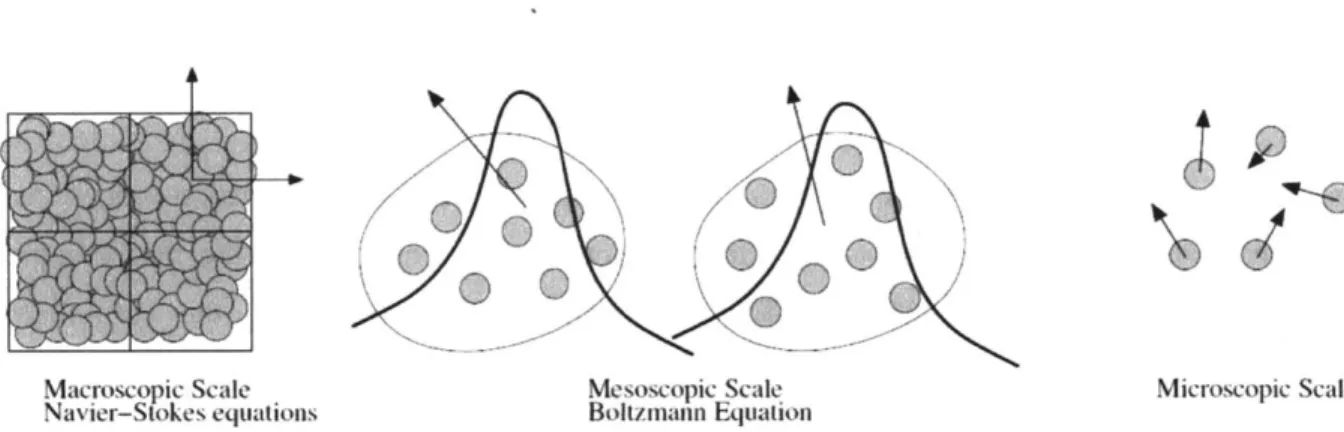
As we could generalize for the universal approaches to solving the transport equations, macroscopic and microscopic views are the two most popular choices. For the macroscopic approach, often called Computational Fluid Dynamics (CFD) simulation, the continuum hypothesis has to be presumed and the nonlinear Navier-Stokes equations are evaluated. To close the solving system, constitutive equations are also included. Different discretization methods need to be implemented and boundary conditions also must be neatly described. In most cases, the algebraic equations have to be solved iteratively until the convergence criteria are reached. Many physical and numerical approximations are made in the problem-solving process, especially for turbulence or other irregular transport patterns. For the microscopic approach, called Molecular Dynamics (MD) simulation, individual particles are well considered, and their local interactions are described as collisions. The nonlinear Partial Differential Equations (PDEs) for solving in macroscopic approach are replaced by simpler ordinary differential equations of momentum conservation (i.e. Newton's second law). Although it is more intuitive, there's also a big problem of memory and storage for numerical solvers. The total number of equations for a single time step is of the same magnitude as the number of molecules of substances, which is really a tremendous burden for the current computers. And it is not even enough because we have to sum up the time range. To make the numerical scheme catch up to the physical process and record the changes of quantities, the numerical time step has to be less than the transient collision time scale, and it leads to the truth that the work to be done might go beyond the capability of the available computers.

The LBM is invented just at the middle of the two scales. It views the whole world in a mesoscopic scale, where individual particle behaviors are analyzed but further collectively integrated in a statistical manner (Fig 2.1). Kinetic equations are solved for the averaged

macroscopic properties, where mass, momentum and kinetic energy are conserved. So the LBM inherits the molecular transport mechanisms, and resolves the tedious work of calculations and storage by summing up to the ensemble properties. These characteristics help achieve the efficiency and relative accuracy of the numerical scheme.

esNoscopic Scale4 Bolt/mnann Equalion A \A towSCOph. Scale Na lir-Stokes equatloII\ SIcroscopic Scale

Figure 2.1. Schematic of different approaches to transport problems.

2.2 Governing equation

As we have mention above, the LBM is directly derived from the LGA by simply replacing the Boolean variable with a distribution function f, and thus the discrete kinetic equation evolves into the following form (Chen et al. 1998, Mohamad 2011).

(x+ eAI, + At) i(x,f) + , (f (x,1)) (2.2)

where f refers to the distribution function for the particle along the jth direction; f j refers to the

collision operator which denotes the rate of change off due to the collision process. If it is written in a continuum form, the equation will be rearranged as follows, known as the Boltzmann equation.

(2.3)

al+ V (fe,)=

Note that it is achieved by approximating both the lattice spacing Ax and the time interval At as small parameters of e and by truncating the second-order term. No external forces are exerted on the system.

Now we should have a close investigation of the distribution function that is oriented in statistical mechanics, and correlates to the macroscopic properties of most interest. Since the stochastic process of collision is really hard to describe, we prefer to find an equilibrium state when the distribution function is independent of directions. It could be achieved after a certain time period because the description of collision process is inherently assumed to distribute all the particles as the same state with the statistical average. From knowledge of molecular kinetics, the Maxwell-Boltzmann distribution equation could be then derived. As we define the equilibrium state, the equilibrium distribution function can be then expressed as,

M

f e=

f,

The summation of the distribution function for all possible states should be defined as unity.

ffeqde=1 (2.5)

Then we can arrive at the expression of equilibrium distribution function by introducing the Maxwell-Boltzmann distribution function (Chen et al. 1998, Mohamad 2011).

eq exp

(eU)2

(2;rRT) 2RT

where p, u are macroscopic fluid density and velocity, respectively; R is the Boltzmann constant;

T is temperature; M is the degree of freedom. To make it convenient for calculation, we use a

Taylor expansion on u and approximate to the second-order (u2), so that it is the same order of accuracy with the Navier-Stokes equation.

peq e

(e.

ee

I

[+ + 2(RT+0 ( _(21rRT (-/ 2RT )-RT 2( RT2 2RT

(2.7)

As we can see from the expressions above, the distribution function is closely related to the macroscopic quantities. By definition,

fi

P= (2.8)

Similarly, we can derive correlations of macroscopic momentum, energy, etc. with the distribution function

fi

pu=If/e, _(2.9)

For an incompressible fluid, the macroscopic density is constant in time and we often assume it as a lattice density po and normalize it as unity, so as to keep up with definition of distribution function. Thus, the macroscopic velocity u can be derived from Equation (2.8) as,

U= _{fe, (2.10)}

At the equilibrium state, all the equations from (2.7) to (2.9) will obviously be also satisfied.

peq= fe= U _{, e,} eq = 2 i (2.11) fi (e -u) 2

where e is the internal energy, and according to kinetic theory, e = MRT/2.

We could then further simplify the Equation (2.6) by (2.10) into the following form.

c~2

f eq =Pwi 1+ 2+ 4 2 (2.12)

c , 2c' 2c,2

where wi is called weight factor, which is determined by lattice arrangements of the domain; c, is called the lattice sound speed which is derived from kinetic theory by approximating infinite

degrees of freedom (i.e. M -+ oo).

cS = yRT= + RT~f2 (2.13)

where y = cc, = 1+(2/M) is a ratio of specific heat.

In real cases, a velocity vector always consists of three components, and thus we define the magnitude of the lattice sound speed as c = = T

/

.

the governing equation, we normally set the value of c as unity in the calculation, and normalize both the particle velocity e and fluid velocity u by c. Then Equation (2.12) will be rewritten as follows.

feq =pw, (1+3(e.u)+-9(e.u)2

_-u2

(2.14)

2 2

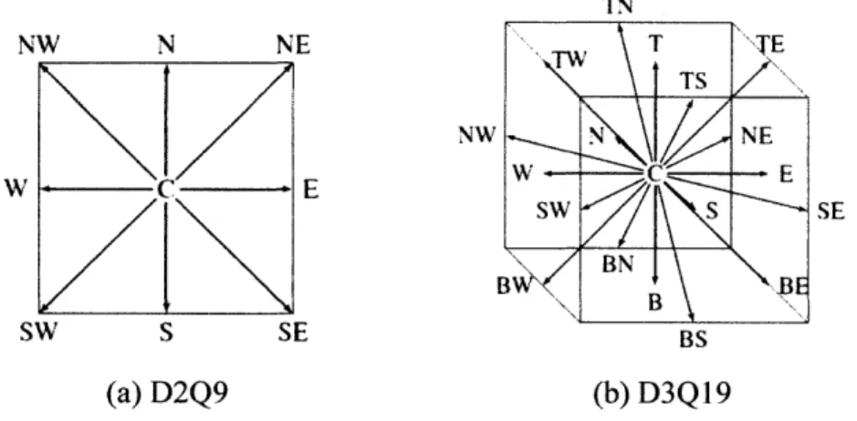
When we need to evaluate the equilibrium distribution functions, we have to first determine the lattice arrangements of the modeling domain. Typically for a two-dimensional (2D) or

three-dimensional (3D) problem, for example, we could set up the linkage of neighboring lattices as depicted in Fig 2.2. TN NW N NE T 'E TS NW NE W C E WE

ISW

Figure 2.2. Schematics of the lattice arrangements in 2D or 3D cases.

Note that commonly for the notations of the lattice arrangements in the LBM, a terminology is often used as DnQm, where n refers to the dimension of the problem (n = 1 for ID problem; n =

2 for 2D; and n = 3 for 3D) and m refers to the degrees of freedom for particle velocities (same as M).

For the D2Q9 model, each lattice (denoted as center C in Fig 2.2 (a)) is closely connected with 8 neighbors and the whole system is categorized into 3 parts: centered lattice itself (C), orthogonal sublattices (N, E, S, W) as well as diagonal sublattices (NE, SE, SW, NW). To obtain the weight function wi, He & Luo (1997) use a third-order Hermite formula to approximate the summation in Equation (2.11). Abe (1997) assumes w, has a simple truncated functional form based on ej. And both reach the same results as follows.

w, =4/9 e = (0,0) ie{C}

, = 1/9 e, =(0,

i)

W, =1/36 e, =( i, i) i e {NE,SE,SW,NW}

For the D3Q19 model, each lattice (denoted as center C in Fig 2.2 (b)) is closely related to 18 neighbors and the whole system is also categorized into three parts: centered lattice itself (C),

primitive sublattices (N, E, S, W, T, B) with a distance of one lattice interval to the centered node, as well as secondary sublattices (NE, SE, SW, NW, TN, TE, TS, TW, BN, BE, BS, BW) which are nearly one half of the lattice intervals away from the center. Weight function values can also be derived by the same methods mentioned above.

W = 1/3 e, = (0,0,0) _{i E {C}}

w, = 1/18 e, =( 1,0,0),( i,o,0),( ] 0,0) i e {N,E,S,W,T,B} (2.16)

1w,

i),(o, i, i)

{NE,SE,SWNW,TN,TE

TS,TW,BN,BE,BS,BW}

Since the collision operator closely relates to the distribution function and we know the function values at the equilibrium state, we can then use a Chapman-Enskog expansion on the collision term and approximate it with the local equilibrium distribution function values to second-order

accuracy.

O ~ ~ ~ f

fi

")e ( "'+( (2.17)

As we have known from the definition that collision process cannot happen at the equilibrium

state, we have: 92 ( "c)=0. Then we will arrive at a linearized collision operator, and Bhatnagar, Gross and Krook (need date), as well as Welander (1954) both introduced a simplified model for that. The collision operator is replaced as,

1, (f e -f; ) (2.18)

where r is denoted as the relaxation factor, referring to the rate at which the local particle distribution approaches an equilibrium state.

From the expression above, we notice that the collision operator also obeys the conservation laws for macroscopic properties. This can be easily proved if we plug Equation (2.8) -(2.11) into (2.18), and sum up the total N lattice nodes.

1 , = 0, , e, = 0 (2.19)

N N

The Boltzmann equation (2.3) can be then rewritten in either a continuum or a discrete form.

'

+V(f~e,) (f -f;) (2.20)

at Ir

f,(x+eAt,t+At)- f (x,t)=

(fe

To relate the relaxation factor to macroscopic properties, we can multiply Equation (2.20) with zeroth order or first order of particle velocity u, and then sum them up in all possible directions, which coincide with the continuum mass and momentum conservation equations listed below for an incompressible fluid.

+ V(pu)= 0 (2.22)

at

+ V(puu) = -Vp + vV2u (2.23)

at

The pressure term in LBM can be obtained from the Equation of State (EOS) p = pRT.

p =cp = p/3 _(2.24)

When we compare with the incompressible Navier-Stokes equation, the relaxation factor can then be correlated with the normalized macroscopic kinematic viscosity v in the form.

Similarly we can extend the correlation to the energy equation, where the relaxation factor depends on thermal diffusivity a.

z = 3a+0.5 (2.26)

To obtain a higher-order accuracy scheme for the collision operator, the Multi-Relaxation-Time (MRT) model has been proposed. For example, Ginzburg (2005) invented the Two-Relaxation-Time (TRT) model, which splits the distribution function into a symmetric and an asymmetric part. Different values of relaxation factor are imposed on the two parts, thus enhancing the accuracy and improving the numerical stability of the overall results.

2.3 Boundary conditions

In the macroscopic approach, the setting of the boundary conditions is more like an intuitive process, because the continuum hypothesis helps to establish the no-slip (tangent velocity equal to zero) and no-flux (normal velocity conserved) conditions at the wall. But in the LBM, the boundary condition issue arises because the continuum framework does not have a counterpart. And many theories in the area of boundary conditions are proposed, of which the bounce-back mechanism stands out for its simplicity (Chen et al. 1998, Mohamad 2011).

The bounce-back mechanism, as is known from its name, mainly implies that an upstream particle moving towards the solid boundary will bounce back into the flow domain with conservation of mass and momentum. It is used to model solid stationary or moving boundary condition with no-slip velocity, and in application for most cases, solving the problem of flow over obstacles.

There are two different schemes to implement the bounce-back conditions depending on the lattice arrangements on the boundaries, and they have different orders of accuracy in approximation (as is shown in Fig 2.3). The first-order scheme suggests that lattice nodes could be directly placed on the boundaries, while the other suggests that the lattice nodes could be

placed so as to make the solid wall halfway between interior and boundary lattice nodes. Since the lattice spacing is normally uniform, by analogy to the finite difference scheme, we can achieve 2nd-order accuracy boundary conditions.

* 0 0 0 0 0

* 0 0 0 0 0

FirIst-ortnIr -il miic IL error Seco 1li d- ordI l n miei l e i (or

Figure 2.3. The two different schemes to implement bounce-back boundary conditions.

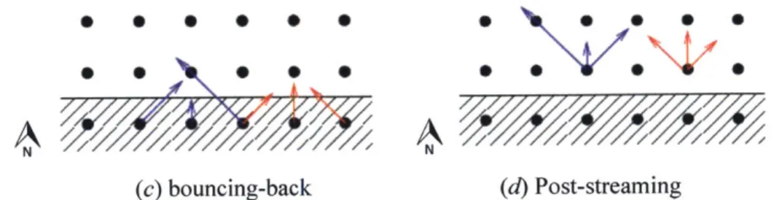
For the second scheme implemented in the D2Q9 framework, the process of bouncing back could be visualized as follows. Firstly, when the upstream particles carrying their lattice-averaged velocities move toward the wall, they will propagate their kinematic properties to the downstream 'virtual' particles residing in the boundaries (Fig 2.4 from (a) to (b)). But since the wall cannot sustain any fluid particles, it forces the mass moving backward to their origins with the same properties at the same orientations (Fig 2.4 from (c) to (d)). In the process, both mass and momentum are conserved.

* 0 9 0 0 0

* 0 0 0 S

I,

*

(a) Pre-streaming (b) Streaming

0 0 0 0 0 0

N N

(c) bouncing-back

Figure 2.4. Bounce-back process in determination

(Upwind direction is from north).

/Z/

(d) Post-streaming

of the second-order boundary conditions

If we take the center node (i, J) with blue arrows in Fig 2.4 as an example to derive the

mathematical expressions for the bounce-back scheme (ith node along horizontal direction, j

node along vertical direction, we have:

f (ij)= f (i, j)= f, (+1 1)

ANW j) E fSE

(2.27)

The derivation of the bounce-back expressions for the D3Q19 from the D2Q9 relations is straightforward and the only difference between the two models is the number of counterparts that have to be set.

When the solid wall is no longer stationary, particles on the boundary should retain the same velocity with the moving solid, because fluid particles cannot sustain any of the shear stress on themselves. And then we can equate the moving boundary velocity Ubc with the macroscopic velocity of the boundary nodes u.

u = Ife, = _u., (2.28)

In some problems, the outlet velocity is not known. To obtain a reasonable periphery boundary condition, a linear extrapolation scheme is often used for the unknown distribution functions on the boundary lattice nodes.

37

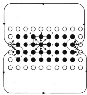
When we'd like to impose a periodic boundary condition, for example, the flow region is just repeating, we should set up the distribution function values on the left boundaries as the same with the function values on the right, shown in the figure below.

00000..000

Figure 2.5. Schematic of periodic boundary conditions implemented by the LBM.

2.4 Numerical Stability

In a real case, for example, if fluid problems are to be solved, we need to set up numerical cases that are similar to physical ones. To achieve that, geometric, kinematic and dynamic similarity must be preserved so as to keep the main characteristics of the flow field. Generally, we will construct a dimensionless counterpart between physical and numerical situations, which is known as the famous Reynolds number (Re). In the physical world, it is more intuitive to find a characteristic length scale (L), known freestream velocity (u) and fluid kinematic viscosity (v) to express Re. And in the LBM, since density and sound speed are both normalized into the lattice form, we need to define the lattice velocity (U) and the lattice viscosity (v) both in dimensionless form. Then a connection on Re is made between the two situations (Kundu et al. 1990, Mohamad 20 1).

In area cae, fr eampe, f

flid robemsare

o

b

soved

we

eedto

et p

nuerial ase

Reh, = Re

uL UN (2.29)

V V

Where N is the number of lattice nodes in the direction of the characteristic length.

During the derivation of the governing equation in the LBM, incompressibility of the fluid is presumed in the macroscopic world, and it should be preserved in the framework of the lattice world as well. The criterion for that is the range of Mach number (Ma), defined as the ratio of fluid velocity and sound speed, which is less than 0.3. For the counterpart in the LBM, values of the lattice velocity must be chosen within the same limits, as:

Ma = < 0.3 (2.30)

C

Since the lattice sound speed has been defined as the normalized value, the lattice velocity should not be larger than 0.3 to sustain the numerical stability. Typically, U is often set at the scale of 0.1-0.2 to reduce the round-off error.

Another constraint for the numerical stability comes from the setting of the relaxation factor, which is closely related to the macroscopic viscosity. As is shown in Equation (2.25), if the value of the relaxation factor is below 0.5, the macroscopic viscosity will be negative, which is unreasonable in a real case. And if it is just above but very close to 0.5, there will be also possibilities of obtaining instable solutions. So it is important to be really careful in choosing the value of that term, especially in high Re flow (turbulence). Considering the normal range of U and r, the number lattice nodes will be very large, thus increasing the computational cost.

2.5 Concluding remarks

In recent years, the Lattice-Boltzmann method (LBM) has developed into an alternative and promising numerical scheme for simulating transport problems and modeling the physics in fluids (Chen et al. 1998). The scheme is particularly successful in fluid flow applications

involving complex boundaries, which is commonly seen in building simulation fields. Unlike the conventional CFD methods dealing with simplified NS equations and the MD method coping with individual particle behaviors, LBM is a hybrid, for its "duality" in between continuous and discrete natures. The discrete nature shows up in its construction of kinetic models where the fundamental physics of microscopic processes is well explained. LBM also has its continuous nature in that the principle focus is on macroscopic behavior described by statistically-averaged functions. The two natures are connected by the mesoscopic kinetic equations that enforce the macroscopic average properties derived out of LBM satisfy the desired macroscopic equations. The connections here are reliable at the basic premise that the macroscopic dynamics of a fluid is the result of the collective behavior of many microscopic particles in the system and that the macroscopic dynamics is not sensitive to the underlying details in microscopic physics (Kadanoff 1986).

The hybrid nature of the LBM introduces three important features that distinguish it from other numerical methods.

The most attractive characteristics lie in its computational efficiency. By focusing on averaged particle behaviors, LBM avoids solving the equation of motion for each particle as in MD simulations. By inheriting the advantages of a discrete kinetic model, including linear convection operator, easy implementation of boundary conditions, and fully parallel algorithms, LBM avoids solving nonlinear high-order PDEs and using discretization methods to achieve numerical solutions. Especially for its fully parallel nature, implementations of LBM solver on parallel computers are relatively easy, because particle motion is evaluated by neighboring nodes in the vicinity and can be decomposed locally over many processor cores, which largely enhances the efficiency of the numerical scheme. Furthermore, the LBM utilizes a minimal set of velocities in lattice space (Chen et al. 1998), and thus reduces the continuous Maxwell-Boltzmann equilibrium distribution into finite discrete moving directions, so that transformation from microscopic distribution functions to macroscopic quantities is greatly simplified into algebraic calculations.

Second, the pressure field is easier to obtain in the LBM compared with conventional CFD methods. In contrast, CFD methods deal with coupled equations (continuity equation and the equation of motion) to solve for the velocity and pressure field, which leads to numerical difficulties requiring decoupling and iterations. But in LBM, pressure field is calculated by the equation of state where macroscopic properties are pre-calculated with distribution functions.

Third, complex boundaries are easily implemented using bounce-back mechanism. No boundary equations (no flux and no slip on the boundaries) are required to solve as in conventional CFD methods, thus increasing the computational speed when a large amount of complex geometries are evident in the modeling domain.

Chapter 3

Validation of Lattice-Boltzmann method in wind field modeling

In the former chapter, the Lattice-Boltzmann Method is introduced to solve the transport problems and its advantages over other computational methods are explained, especially from the perspective of wind field modeling for urban canyons and their neighborhoods. In order to validate its merits in simulating wind fields in a fast and relative accurate manner, sample case studies are performed for the velocity and pressure fields, which are the two primary indicators of wind field. Comparisons will be made between LBM simulation results and experimental data (wind tunnel results) as well as CFD commercial tools (scSTREAM). LBM is coded in C#, which is source-friendly to a Rhino-based working environment and could be easily integrated in designers' workspace and post-possessed by Excel and Matlab tools.

3.1 Wind velocity field 3.1.1 Case description

A case study is conducted with a single building in the modeling domain (as is shown in Fig 3.1). The goal of this case study is to validate the LBM performance in calculating the wind velocity field with respect to the wind tunnel experiments constructed by the Architectural Institute of Japan (Shirasawa et al. 2003). In order to compare the results with experimental data, building size and wind field parameters are set to match the experimental settings, which are further explained as follows.

In the physical domain, a single building is located in the center of the domain, with a length of 50 mm, width of 200 mm and height of 200 mm. The upwind velocity distribution satisfies the power law along the vertical direction, which is the typical setting of inlet wind profile in ASHRAE Handbook of Fundamentals (ASHRAE 2013), with the maximum value of 7.84 m/s at

the top of the physical region (maximum height of 1000 mm), and wind speed is uniform in a horizontal plane. The expression of the wind velocity is shown as follows:

u(z)= 7.84(z / 1000)'/ (3.1)

Where z is the height (unit: mm) and u is the wind velocity (m/s) at a certain height.

In the numerical domain of LBM, the building is centered in a cube of 2000 mm in both horizontal directions and 1000 mm in the vertical direction. To keep the dynamic similitude for the LBM model, Equation (2.28) is used to set up the gridding and relevant parameter values, and in the process, the numerical stability analyzed in Chapter 2.4 is also carefully considered. For example, to achieve the incompressibility of the fluid, the lattice velocity (U) on the top of the domain is set as 0.1, which represents the physical value of 7.84 m/s in the real world. In this case, after we calculate the Reynolds Number (Re), we will find that high Re flow takes place in the modeling region, and large numbers of the lattice nodes have to be set to ensure the numerical viscosity is within the safe range of stability. For instance, a uniform gridding is utilized with an interval of 12.5 mm, and thus there are 161 lattice nodes including periphery boundaries in both the x- and y-direction (defined in Fig 3.1), as well as 81 nodes in the z-direction. Roughly 2 million lattices are involved in the calculation.

4b

z 4b