DYNAMIC SCHEDULING IN
AIRLINE OPERATIONS
.iJ. Akel
Moppppp-MASSACHUSETTS INSTITUTE OF TECHNOLOGY Flight Transportation Laboratory
Technical Report FTL-R67-1
December 1967
DYNAMIC SCHEDULING IN AIRLINE OPERATIONS
O.J. Akel
This work was performed under Contract C-136-66 for thbe Office of High Speed Ground Transport, Department
TABLE OF CONTENTS Page Chapter 1 1.1 1.2 1.3 1.4 1.5 1.6 1.7 1.8 Chapter 2 2.1 2.2 2.3 2.4 2.5 2.6 2.7 2.8 2.9 Chapter 3 3.1 3.2 Chapter 4 4.1 4.2 4.3 4.4 Chapter 5 5.1 5.2 5.3 5.4 Chapter 6 6.1 INTRODUCTION Background
The Scheduling Process The Scheduling Environment Types of Schedules
Purpose
Content of the Study Preview to Chapters Validation
DEVELOPMENT OF DISPATCH STRATEGIES Motivation
The Fare
Fixed Operating Costs
The Passenger Delay Penalty Selecting a Departure Time Total Return per Flight
Average Return per Passenger The Marginal Concept
Coupling Consideration
TEE TWO STATION PROBLEM The DYNAMO Model
The GPSS II Model
THE NINE-STATION PROBLEM
Model Structure and Operation Dispatch Decision Rules
Output Format
Discussion of Runs THE AIR TAXI PROBLEM
Model Structure and Operation Dispatch Decision Rules
Output Format
Discussion of Runs
THE ADAPTIVE DECISION MODEL Introduction 11 11 14 14 15 18 20 23 24 29 37 37 42 76 78 81 84 87 95 95
TABLE OF CONTENTS (Continued) 6.2 6.3 6.4 6.5 6.6 6.7 Chapter 7 7.1 7.2 7.3 7.4 Bibliog raphy Model Operation
The Learning Process Decision Heuristics
The Dispatching Threshold Discussion
Summary
SUMMARY AND CONCLUSIONS Summary
Conclusions
Computation Time
'uggestions for Further Study
Page 97 99 101 102 108 119 121 121 122 127 127 129
LIST OF FIGURES
Page
2.1 Return Function Components 19
2.2 Cumulative Return Function 19
2.3 Optimization of Total Return per Flight 22 2.4 Optimization of Average Return per Flight 22
2.5 Average Return per Passenger 25
2.6 Effect of Non-uniform Arrival Rates on
the Return Function 25
2.7 Daily Arrival Rate Distribution 28
2.8 Time Horizon for the Marginal Return
Criterion 28
2.9 Aircraft Disposition Components for
Decision Coupling 32
2.10 Relative Passenger Demand Component
for Decision Coupling 32
2.11 Dispatching Heuristics for Decision
Coupling - Two Station Shuttle 36
3.1 Daily Variation in Average Interarrival
Time 43
3.2 Passenger Interarrival Times - Poisson
Process 43
4.1 Daily Demand Variation Multiplier 53
4.2 Daily Total Demand Distribution 53
4.3 Fare/Cost/Flight Time Structure: Nine
Station Network 55
4.4 Effect of Delay Penalty Constant 63
4.5 Effect of Passenger Guarantees 67
4.6 Effect of Time Horizon 69
4.7 Effect of Fleet Size 73
5.1 Helicopter Air Taxi Service 77
5.2 Daily Variation in Demand to and
from Airport 80
5.3 Fare/Cost/Flight Time Structure 82
6.1 Aircraft Disposition Components for
Decision Coupling 107
6.2 Relative Passenger DemandComponent for
LIST OF FIGURES (continued)
Page 6.3 Passenger Demand Distribution after 5 110
Day Run
6.4 Probability Measure Changes
Resulting from Past Demand Experience 111
6.5 Cumulative Net Revenues 112
6.6 Cumulative Passenger-Minutes Wait 114
6.7 Net R'turn Function 117
LIST OF TABLES
3.1 Run Summary, Nine-Station Model - Dynamo 40 3.2 Run Summary, Two Station Model - GPSS II 46
4.1 Run Summary, Nine-Station Model 61
5.1 Run Summary, Air Taxi Model 86
6.1 Run Summary, Adaptive Decision Model 109
CHAPTER I
INTRODUCTION
1.1 Background
Although air transportation has been characterized
by rapid development in vehicle design and performance, methods of airline management in the area of vehicle
scheduling and control have advanced at a much slower
pace.
Because of high costs of operation and the
pres-sures of current competition and government controls,
effective and efficient use of aircraft is becoming an
increasingly essential objective. The goal is to
achieve an optimal balance between net revenue to the
airline and improved level of service to the customer. Improved return implies higher load factors and air
-craft utilization whereas improved passenger service
necessitates reduced waits and increased frequencies.
These are often conflicting aims. New techniques must
be mobilized to give management more useful and
adap-tive methods of operating and controlling an air
of a very short-haul high density transportation
sys-tem will lead to more demand responsive approaches. It is with this motivation that this study of dynamic
dispatching strategy is undertaken.
1.2 The Scheduling Process
The decision-making process by which the system operates is called a scheduling strategy. Given the
present system state in terms of accurate real time
information concerning demands, passenger waiting
time, vehicle availabilities, etc., and some short
term expectations of future system states, a set of
operating rules is established which determines the
transportation system response. This set of rules, or strategy, always exists, either explicitly in the form of management policy directives, or implicitly in the form of the experience and intelligence used
by the dispatcher. There are a wide variety of strat-egies available, each of which uses certain information
1.3 The Schedulinq Environment
In scheduling, it is convenient to distinguish
between short-haul and long-haul type operations.
Generally, circumstances inherent in longer haul
opera-tions make scheduling a simpler problem. These
in-herent features include the lower volumes encountered
and the greater degree of advance preparation for the
trip on the part of the passenger.
Short-haul traffic, on the other hand, usually involves larger volumes and little or no advanced
prep-aration by the passenger. Included in the latter is
the commuter service to and from metropolitan centers
and the general collection and distribution problem
between adjacent communities. Of course, a critical element in the scheduling environment is the
uncertain-ty associated with demand. The uncertainty exists with
respect to the total volume of traffic as well as the
arrival distribution of individual passengers
through-out the day.
Although the passenger places emphasis on speed,
in a short total elapsed time, i.e. the time from being ready to leave his home or office until the time when he arrives at his ultimate destination. Infrequent departures can result in unacceptable waiting times for many passengers who will conse-quently seek alternative modes of transportation. Excessive frequencies, on the other hand, burden the airline with unnecessary operating costs and over-capacity.
1.4 Types of Schedules
Basically, service schedules may take one of three forms:
a) Fixed Timetables
b) Dynamic or demand schedules c) Mixtures of (a) and (b)
The fixed schedule, or timetable, is most commonly used, not only by airlines but also by intercity bus lines and passenger trains. Fixed timetables may be desirable for the passenger if it is compatible with his travel plans and he is able to secure a reservation.
From the operator's standpoint, a fixed timetable allows advanced planning and scheduling of resources. Through the use of historical data and knowledge of competitor actiondeparture times can be established which result in better operating efficiencies over
the system. However, once scheduled, a flight must be operated regardless of adverse economic implica-tions. Uncertainties in demand, therefore, can cause poor load factors and sub-optimal operation. While the passenger may want to be assured of departure times, perhaps less rigidity in timaes would permit an overall superior service.
At the other extreme lies the pure dynamic or demand type schedule where departures are governed by some function of the current state of the system. In its pure and unrealistic form dispatches would be made by a decision rule based only on some economic function of the number of passengers and their waiting times.
It is in the third type where the greatest interest lies. An example is the Eastern Airlines shuttle, where aircraft departures are scheduled at fixed times with
supplementary aircraft accomodating the overflow. The popular appeal of this type of service is evi-denced by Eastern's success in the shuttle. In a sense this is a demand schedule with a guarantee that
pas-senger waiting time will not exceed some maximum
value. With an uncertain operating plan of this type, the system must have excess resources in order to meet the guarantees during peak or above average traffic. Thus, lower efficiencies may result with correspond-ingly
trave
1.5
higher costs. However, better service for the ller is presumably assured.
Purpose
The purpose of this study is:
1. To construct simulation models to represent several typical airline situations.
2. To formulate various dispatching criteria compatible with the environments modelled. 3. To demonstrate the use of the simulation
models in:
(a) Evaluating the formulated decision criteria
(c) Determining capacity and aircraft requirements for a given system. 4. To explore other uses for the models.
1.6 Content of Study
In this study primary attention is focused on the dynamic schedule. In effect no prior schedule is assumed to exist and departures are governed basically by some economic consideration. Numerous such criteria are examined and tested on various model situations. In all cases there are overriding upper and lower
bound heuristics which serve to limit passenger delays to a predesignated range.
Initially a mathematical approach was investi-gated with an attempt to apply decision trees and dy-namic programming to the problem. These did not appear to be feasible for problems of practical size, however, and so attention turned to simulation. Simulation per-mitted the evaluation of different decision rules under different conditions. Further, it simultaneously cre-ated a good timetable. That is, for an assumed travel demand, use of the model generated a departure schedule
conforming to the policy objectives built in. The demand assumption is reasonably valid as there usually exists a host of data on which to base expectations.
Policy objectives are real factors in the scheduling decision but may vary considerably as the situation
and relative competitive position changes. The sen-sitivity of these heuristics on overall system per-formance was examined by evaluating controlled changes. Three individual situations were modelled.
1. A two station shuttle problem 2. A nine station problem
3. A twenty station air taxi problem
1.7 Preview to Chapters
In Chapter 2, the various factors which enter into the decision to dispatch an aircraft are con-sidered. From these factors several criteria evolve which are later used in the simulation models.
In Chapters 3, 4, and 5, the three problems listed above are discussed. Pertinent features of the struc-ture and operation of the models are explained. The Chapters conclude with a discussion of the runs and
the observations of significance.
In Chapter 6, the 'adaptive' approach to aircraft dispatching is considered. In essence the air taxi model of Chapter 5 was reprogrammed to permit past experience with respect to demand to be absorbed and
later used to update the dispatching criteria.
DYNAMO and GPSS II simulation languages were used and runs were made on the M.I.T. Time Sharing System.
1.8 Validation
The two station and nine station problems are completely hypothetical. However, costs, fares, flight times, etc. used are considered compatible and realistic for such operations. Though no formal validation was possible the results seemed to conform with expectations of experienced individuals.
The twenty station air taxi problem was modelled from an operating helicopter service company in the area. Although here, too, no formal validation was conducted, various company executives were unanimous
in asserting that the model conformed very closely to their actual operations. Again, it may be stated that the results, in general, were both reasonable and realistic.
CHAPTER 2
DEVELOPMENT OF DISPATCH STRATEGIES
2.1 Motivation
In the operation of an industrial enterprise,
be it factory or airline, it is typical to set a
specific profit objective as a corporate goal.
Whereas price, or fare, is usually fixed by either
supply-demand or else by government regulatory
agencies, cost of operations, as influenced by
quality of service and type of equipment, is in the
realm of management policy and control.
Operating at lower echelons there may be other
non-economic criteria, represented in different di-mensions, but, nevertheless, contributing in some way
to the specified overall economic objectives. In an airline these sub-objectives may be expressed as
passenger delay or goodwill loss minimization, or as aircraft utilization and load factor maximization.
We may enumerate many others while never losing sight
of their overall economic implications.
may be termed "heuristic" to differentiate them from
the true optimal set of rules. The heuristic approach
does not guarantee an optimal departure time but
rather aims at achieving 'improved' performance.
Through the facility of a simulation model,
heuris-tics may be continually modified and observed until a practical and usable rule is evolved. Further
simulation can be used to test the sensitivity of
the decision variables of a given rule and thereby'
assess the value of added refinements.
The process of making a dispatching decision can be considered as a sequence of fundamental
ques-tions and a deduction based upon the answers.
There-fore the development of a useful heuristic involves breaking down the process into basic elements and
applying them systematically and consistently. In effect the attempt is to simulate the thought
proces-ses of an experienced dispatcher, the contention
being that he will make good decisions most of the
time. Poor performance is largely attributed to
systemati-cal reasoning, and to masses of unassimilated data which tend to be more confusing than helpful. With the development of logical heuristics and their dili-gent application by computers immune to such pressures, consistently superior performance should be realized.
In the simulation models of this paper, a number of different binary-type (go - no go) dis-patching rules are developed and applied, more or less simultaneously. That is to say that only one of a sequence of rules need be satisfied to author-ize a departure. Most of these may be classified as upper or lower bound constraints such as rules which cause an immediate dispatch when the maximum aircraft capacity is reached or which prevent an absurd delay time when only a few passengers are on hand.
However the major criterion is an economic objec-tive function and embraces three components:
1. The accumulated fare
2. The fixed cost of operating the flight 3. A self-imposed penalty for delaying
2.2 The Fare
A fare structure is defined for each flight net-work considered. This is taken here to be a constant
for a particular sector (or city-pair); special group
excursion, mixed classes, children rates as well as
round trip discounts are not considered. It would
not be difficult to build fare variations into the
models, but these would not contribute significantly
to the conclusions and are omitted in the interest
of simplicity.
2.3 Fixed Operating Cost
For each sector a direct cost of operating a
flight is incurred regardless of the passenger load.
This cost reflects the trip expenses of fuel, crew,
fees, etc., a maintenance and a depreciation allow-ance. For each sector it may be considered to be a
fixed quantity which we will take as some multiple
of the passenger fare. This cost may not always be
fixed, as for example when the models are being used
to determine fleet size. Typically the same
Therefore the larger the fleet size, the smaller the maintenance burden each aircraft is called upon to bear. Maintenance costs constitute about 15% of the total fixed cost. Of course the option to subcontract maintenance nearly always exists and this would vali-date the assumption of fixed operating cost.
2.4 Passenger Delay Penalty
Passenger delay penalty is an essential factor in the dispatch decision criteria. Were it not in-cluded, the dispatching decisions would be nearly trivial, since with no penalty associated with pas-senger delay, the optimum strategy would be to dis-patch only when full, except insofar as the aircraft might be needed elsewhere.
The delay penalty is a realistic factor imply-ing both a short range and a long range consideration. In the short range, delaying a passenger excessively may mean a cancellation, thus losing him to a com-petitor or possibly to an alternate mode of trans-portation. The longer range consequence results from loss of go3will. This may cause the passenger to
intentionally avoid the airline sometime in the future
because of some unpleasant previous experience.
Quantifying this function is no trivial task.
Different people view this with varying degrees of
importance. Indeed, the same person may well assess
it different val .es depending on such variables as
the time of day, the particular station location,
or according to the activities of the competition.
Looked at from the passengers viewpoint, it is generally agreed that the penalty is not linear in
waiting time but varies as some positive power
(greater than one). It is assumed here that a
pas-senger detained for two hours is likely to be more than twice as disturbed as the passenger held up only one hour. Secondly, it Eeems likely that the penalty
should be different depending upon the projected
length of the journey. A passenger who must wait one
hour for a flight of hour duration is apt to be more
upset than a passenger who waits the same time for a
These facts are combined into a function by having
the delay penalty vary inversely as the fare and
directly as the square as the waiting time. A
constant weighting factor, KD, reflecting subjective
values is included to complete the function. The
delay penalty expression used in the simulation
models is:
Delay penalty = n - KD
.(t)
2 (2.1)f 2)
where n = number of passengers waiting
t = longest waiting time
f = fare
Of course, it may also be argued that delay is re atively insignificant up to a given threshold or a point of discontinuity, beyond which further delay
has extremely high cost. This threshold would repre-sent the point at which the delay causes the passenger
to miss a business appointment or a flight connection,
etc. Clearly, this varies consideLably and is most
difficult to predict. Therefore, for the purpose of
2.5 Selecting a Departure Time
For a given objective function, optimization
is a relatively simple task when the function is
continuous and differentiable. What we would really
like to have is a continuous function with a single
global peak. However in reality, there is a stepwise
discontinuous curve since the function is made up of
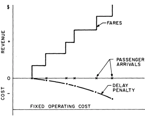
components shown in Figure 2.1. As discrete arrivals
occur, a fare is collected. This is represented as
a step function with the unequal intervals reflecting the
randomly occurring interarrival times. Simultaneously
with the arrival of the first passenger a delay penalty
starts building up. Each arrival is a point of
dis-continuity and the slope of each segment becomes pro-gressively more negative, reflecting the cumulative
effect of an increased number of passengers waiting. Superimposed on these curves is a third signifying the
fixed cost of operating the flight. These three
com-ponents are combined in Figure 2.2 to show the single
cumulative return criterion, or objective function.
FARES 2 PASSENGER ARRIVALS 0 DELAY PENALTY
FIXED OPERATING COST
FIGURE 2.1: RETURN FUNCTION COMPONENTS
CUMULATIVE
o + RETURN
FUNCTION
O
to the discrete points of arrival, it may be easily concluded that more than one maximum is possible. This would be conceivable, for example, when a large number of passengers are waiting (and therefore the slope of the penalty curve is steep) and a relatively long period elapses before the next passenger arrives. Dispatching at this point would yield a sub-optimal
result if the departure was followed by several arrivals in quick succession. Some expectation of future traffic is evidently required to assist in making optimal de-cisions.
One may choose to examine two forms of the objective function:
1. Cumulative return per flight 2. Average return per passenger
The following sections show some analytical considera-tions of these two cases in determining optimal dispatches when the arrival rate is uniform.
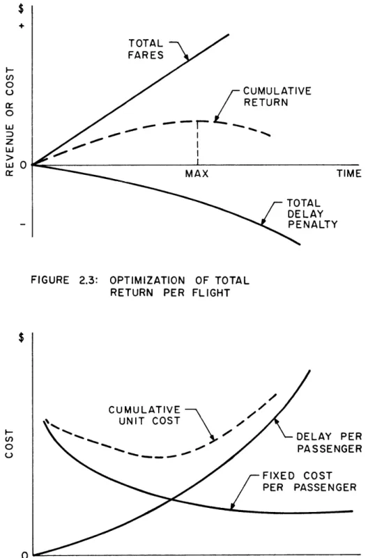
2.6 Cumulative Return per Flight
First consider the relation for total return per flight
Return R = nf - cf- , (T) where f = fare per passenger
n = number of passengers =A t
c = fixed cost as a multiple of fare
KD = delay penalty constant
T = average waiting time = t/2
t = passenger arrival rate, assumed constant over t for this analysis
\tKD
R = tf - cf - (t/2)2 ,f Therefore R = tf - cf - KD 3 4f (2.3) Dif ferentiating dR = f - 4f 3K .t= t = 0Therefore optimal departure time to arrival rate is t 4f2 0 3KD , for a constant 2f 3 (2.4)
Note that in optimizing total return, the fixed cost is
irrelevant. In effect the revenue from fares is being
off-set by the increasing value of the delay penalty. When the (2.2)
TOTAL FARES
W
0 0 z LdJ MAX TIME LTYFIGURE 2.3: OPTIMIZATION OF TOTAL RETURN PER FLIGHT
CUMULATIVE UNIT COST
DELAY PER PASSENGER
TIME
FIGURE 2.4: OPTIMIZATION OF AVERAGE RETURN PER PASSENGER
CUMULATIVE RETURN
total fare accumulated per unit of time is equal to
the delay penalty build up per unit of time, the optimal departure time is at hand. See Figure 2.3.
2.7 Average Return per Passenger
From equation 2.2, the average return per pas-senger is derived: Return/pax = R = R/n = - cf -n N~ cf KDt 2 f 4f nKD2(T) nf (2.5) Differentiating dR cf dt Xt 2 2KDt =0 4f
Therefore the optimal departure time
t'i= 3 2cf2 \KD
Note that in optimizing average return per passenger
the fare is irrelevant. We are offsetting the decreasing fixed cost per passenger as the number of passengers
increases with the increasing delay cost as the time (and passengers) increase. When these two factors are
equal, the minimum cost per passenger obtains. See Figure 2.4. (2.6)
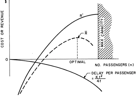
In the absence of a delay penalty, the return
per passenger may be expressed as
R' = f - cf (2.7)
n
Therefore as passengers increase, the average
profit-ability or profit margin increases. Now consider the
effect of a delay penalty. Assuming a constant ar-rival rate, the delay penalty and the total curve
must be represented as shown in Figure 2.5.
2.8 The Marginal Concept
It seems clear that the immediate objective of
an airline should be the maximization of total return,
within the resource constraints, as opposed to maxi-mizing average return per passenger. The latter
cept is analogous to the "full costing" averages
con-sidered in various areas of economics, and as such may
be a perfectly valid parameter in long run considerations.
However in the short run when facilities and
capacities are fixed, and in keeping with the spirit
of dynamic scheduling, a variation of the total return
R
OPTIMAL
NO. PASSENGERS (n) PA SSENGER
I//
FIGURE 2.5: AVERAGE RETURN PER PASSENGER
PASSENGER ARRIVALS
t2
TIME
FIGURE 2.6: EFFECT OF NON-UNIFORM ARRIVAL RATES OF THE
RETURN FUNCTION
economics we may draw the concept of "marginal" returns and apply it to the aircraft dispatching problem.
In considering whether an aircraft should depart at a given time t, or should wait an interval of time
Lt to depart at a time t2, the net contribution to overhead is the difference between the fares derived
from passengers arriving in & t, and the additional
delay penalty incurred by the present passengers waiting until time t2. An incremental penalty can be included
for the waiting incurred by the arriving passengers in & t. The marginal contribution to overhead then
becomes:
MCON =mf _hD n (2)- n + m
f 2Il\2
mf -
n(t2 - t2)
+
m
At2
(2.8)
where m = expected number of passengers arriving in & t n = present number of passengers at t1
If the arrival rate is uniform, the obvious cri-terion for dispatch would be a zero or negative value of MCON. (This would occur at intervals of time dif-ferent from to of Section 2.6. since the incremental
delay penalty of the arriving passengers is computed in a different manner.)
However, with non-uniform interarrival times this may not be the case since a large number of arrivals in a short period of time may quickly reverse the trend of the curve as demonstrated in Figure 2.6.
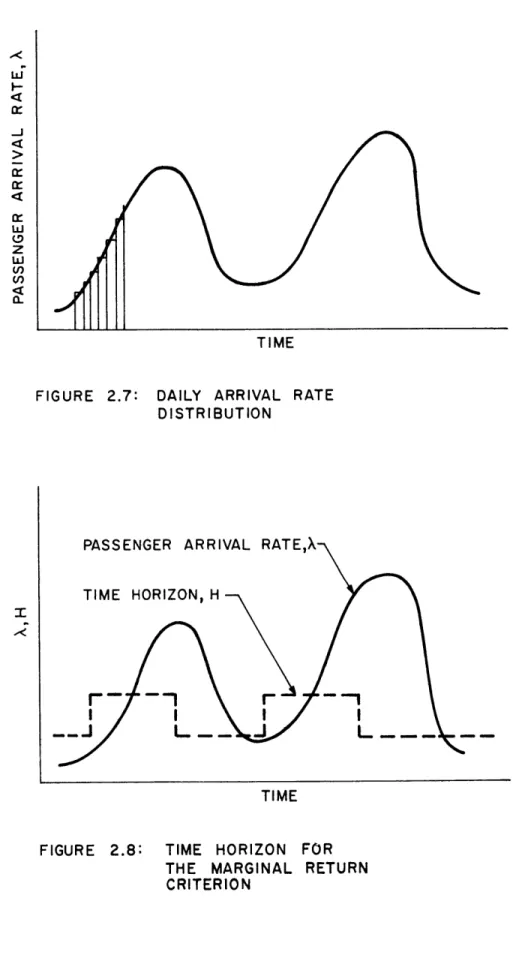
Characteristically demand for commercial air travel fluctuates throughout the day describing in essence a two-peaked curve. Therefore the total daily demand, whatever it may be, will be distributed in the manner suggested by Figure 2.7.
Arrival rates (and interarrival times) are con-sequently functions of the time of day. This point is significant since it invalidates the previous as-sumption that \ is a constant. We must therefore consider it as a time dependent, 'controlled variable' in that it changes throughout the day but in a pre-dictable fashion.
In essence the problem reduces to one of selecting an appropriate time horizon over which to examine the the marginal returns of revenue and penalty. During
TIME
FIGURE 2.7: DAILY ARRIVAL RATE DISTRIBUTION
PASSENGER ARRIVAL RATEX
TIME HORIZON, H --\
TIME
FIGURE 2.8: TIME HORIZON FOR THE MARGINAL RETURN
peak periods, when there is a high probability of acquiring additional passengers by delaying the flight further, to extend the horizon would seem reasonable. Conversely, during slack periods, the value of looking beyond the next few time periods is correspondingly reduced. It is therefore feasible to define a variable horizon whose value changes as a function of the time of day distribution. It may be a simple two valued function (Figure 2.8) or a more complex infinitely variable relation. Therefore in equation 2.8, & t becomes a function of time, H(t).
MCON = mf - n (t + H(t)) - t2 + m H(t)2 (2.9)
4 f 1J
This expression is in terms of quantities readily avail-able to the decision rule at any time in any simulation. If MCON 4 0, then the decision to depart is made at t .
2.9 Coupling Considerations
In addition to the marginal contribution consid-erations of operating a flight from a particular station, it is often of equal importance to look ahead to the
The question is when and to what extent does the state at other stations become significant in the
decision to dispatch a vehicle from this station?
There are basically two separate considerations
of relevance.
1. The first pertains to the current dis-position of the aircraft in the network
2. The second pertains to the passenger/
waiting time states at the stations
involved.
For example, if a decision is to be made whether
to dispatch an aircraft from station A to station B,
the passenger state at B becomes pertinent to the de-cision at A so long as the subsequent dispatch of B's passengers depends upon the arrival of this particular
aircraft from A. That is to say, there are no aircraft
at B or on route to B which could satisfy the expected
demand at B. Clearly with unlimited aircraft in the
system, the dispatch decisions at a particular station
are independent of the system state at other stations.
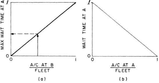
relative location status becomes increasingly im-portant. Consider two stations in a network. From the standpoint of aircraft disposition, the wait time prior to dispatching from A to B may be considered as the sum of two components as determined by Figures
2.9a and b. Assuming equal demand expectations at the two stations, the lesser the proportion of air-craft at A the longer the wait time desirable at A. In this case waiting longer may result in more pas-sengers being carried on the flight, without endanger-ing the subsequent departures from B. On the other hand the greater the number of aircraft at A relative
to the fleet size, the wiser the choice to depart early and thereby make available sufficient aircraft at B to handle the expected demand without suffering an unnecessarily high delay penalty. These two com-ponents may be weighted unequally if considered
neces-sary (e.g. unequal demands at the two stations).
The second factor affecting the dispatch decision concerns the relative buildup of passengers at the
stations involved. Important here are expectations
-31-1 0 A/C AT B FLEET A/C AT A FLEET (a) FIGURE 2.9: (b)
AIRCRAFT DISPOSITION COMPONENTS FOR DECISION COUPLING
Oi 0
r=E (A)PA (B) E (B) PB (A)
FIGURE 2.10: RELATIVE PASSENGER DEMAND COMPONENT FOR DECISION COUPLING
LUJ
H
of daily demand and the relative time of day varia-tions at each station. Consider impending flights
from A to B and B to A. Passengers arrive at some
expected rate with the probability of a passenger
going from A to B being PA(B) and from B to A, PB(A).
Let E(A) be the expected number of passengers
orig-inating at station A during a given time period
As the ratio of PA(B) E(A) _ Expected no. of pax A to B P B(A) E(B) Expected no. of pax B to A
varies, the desirable predeparture waiting time for
flight A-B varies from 0 to some number greater than
one which is governed primarily by policy
considera-tions and published guarantees. See Figure 2.10.
This says that if there is a greater volume of potential
passenger flow from A to B than from B to A in the given time period, all other things being equal, it is in the interest of the airline to delay the flight at A as long as practically possible. Conversely, if
the ratio r is very small, i.e. there are a relatively
larger number of passengers wishing to travel from B
to A, then it may be desirable to dispatch the flight
economic criterion. This is particularly significant in the absence of reliable data on passenger demands and when a given level of service is guaranteed.
The above relative-aircraft and relative-passenger criteria may be combined into some single equation
form with equal or unequal weighting, and applied simultaneously with the economic and upper-lower bound criteria.
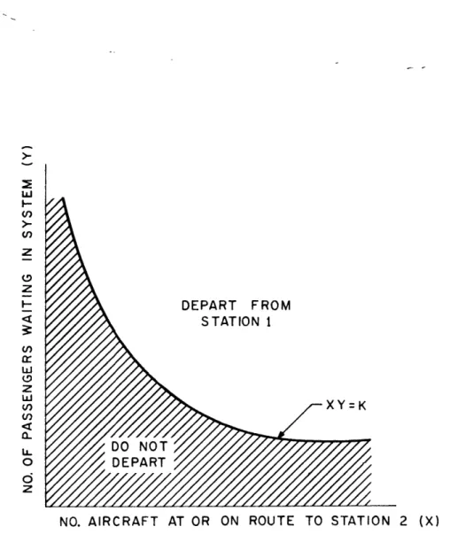
Depending upon the problem at hand, it may often be found that much simpler heuristics are useful. In a two station shuttle, one criteria in the decision rule might be governed by the number of aircraft available to the station and the total number of
passengers waiting in the system. A limit for the product of these two measures is established, and, once exceeded, the aircraft is dispatched. In Figure 2.11 any point outside the shaded area would signal a departure. In effect, this states that if there is a high concentra-tion of aircraft at the other staconcentra-tion, and thus fewer at this station, a greater passenger demand is required
for a departure. The 'establishment of the limit might depend upon the number and capacity of the serviceable
aircraft in the system, route competition, management policies, etc.
-35-w (n Uf) z (9 z I- DEPART FROM STATION 1 () w z w o DEPART ci z
NO. AIRCRAFT AT OR ON ROUTE TO STATION 2 (X)
FIGURE 2.11: DISPATCHING HEURISTIC FOR DECISION COUPLING -TWO STATION SHUTTLE.
CHAPTER 3
THE TWO STATION PROBLEM
3.1 Dynamo Model
Among the initial simple problems considered was the two station shuttle with a fixed number of air-craft pre-positioned at the two stations. The average value of daily passenger demand was considered to be normally distributed. Time of day hourly variations were assumed known, given the daily average and the model was run using three different simple dispatching
strategies.
Dispatch an aircraft:
Strategy 1) When demand is 55 passengers or more (60 for station 2)
Strategy 2) Every three hours after 9:00 AM provided that at least 55
pas-sengers are on hand (60 at station 2)
Strategy 3) Every three hours and anytime passengers waiting exceed the set limit, 55 or 60.
carrying out an indirect optimization of the return equation.
Return = (PW) (Fare) - K(PW)3 - Fixed cost (3.1)
where PW is the number of passengers waiting and the second term is an approximation of the delay penalty.
This model was written in Dynamo, a time driven simulation language. Outputs consisted primarily of a departure schedule with certain accrued parameters of interest carried along.
Of significance are:
TRET Total accrued returns from flights PAXW Number of passengers waiting
LOAD Number of passengers carried on the flight NACG Number of aircraft on the ground
NACF Number of aircraft flying
TPCAR Total accrued passengers carried
Aside from the schedule generated, the parameters tabulated serve a useful purpose. NACG gives a good indication of any over-capacity. Further it might be feasible to adjust departures slightly to realize an
additional saving of one aircraft at a small cost in waiting time. The number of passengers waiting at any particular time, PAXW, is a useful indicator of the
level of service being achieved.
3.1.1 Discussion of Runs
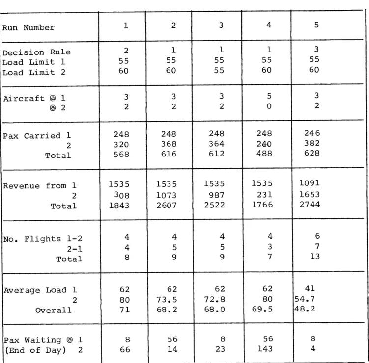
Results of several runs are tabulated in Table 3.1. Runs 1, 2, and 5 are identical with the excep-tion of the strategy used. From the overall return standpoint, Run 5 (strategy 3) is slightly better than run 2 even though four additional flights were required to carry approximately the same number of passengers. The higher delay penalties involved in run 2 offset the fixed cost savings realized in higher load factors. Strategy 2 (run 1) is more difficult to satisfy than the others, consequently
less flights were operated and longer passenger delay times were suffered. This detrimental effect of
strategy is measured by the low associated total return. Runs 2 and 3 examine the sensitivity of the "optimal" passenger load to the overall per-formance of the system. In run 3 the load limit
TABLE 3.1 RUN SUMMARY
TWO STATION MODEL - DYNAMO
Run Number 1 2 3 4 5 Decision Rule 2 1 1 1 3 Load Limit 1 55 55 55 55 55 Load Limit 2 60 60 55 60 60 Aircraft @ 1 3 3 3 5 3 @ 2 2 2 2 0 2 Pax Carried 1 248 248 248 248 246 2 320 368 364 240 382 Total 568 616 612 488 628 Revenue from 1 1535 1535 1535 1535 1091 2 308 1073 987 231 1653 Total 1843 2607 2522 1766 2744 No. Flights 1-2 4 4 4 4 6 2-1 4 5 5 3 7 Total 8 9 9 7 13 Average Load 1 62 62 62 62 41 2 80 73.5 72.8 80 54.7 Overall 71 68.2 68.0 69.5 48.2 Pax Waiting @ l 8 56 8 56 8 (End of Day) 2 66 14 23 143 4
required at station 2 was reduced from 60 to 55. As a result the same number of flights were operated with the same average load factor. However total
return dropped 3%.
In all runs discussed thus far three aircraft were pre-positioned at station 1 and two at station 2. In runs 2 and 4 the effect of pre-assigning all aircraft to station 1 was examined. As no ferry flights are permitted, passengers at station 2 must wait for a revenue flight from 1 to arrive before being accomodated. As a result heavy delay penal-ties were suffered at station 2 as evidenced by the
low return ($1766 versus 2607).
While much can be learned from this model, its limitations are clear. First, there is little room for any degree of sophistication in the decision rules. Secondly, it is difficult to incorporate waiting
times as an element in the decision process. Further it is difficult to expand the number of stations to a realistic level.
-41-These and other considerations prompted a
deci-sion to move to a more powerful and flexible simulation language. Thus the remaining models were written in
GPSS II and run on the MIT Time Sharing System.
3.2 GPSS II Model
This model represents essentially the same
situa-tion as that in Secsitua-tion 3.1, but possesses greater
flexibility in the demand function as well as the
de-cision criteria. Several working versions of this
model were written. The one included herein is the
most advanced from the standpoint of comprehensive-ness. However, from the standpoint of computer time,
it is relatively inefficient; having small time inter-vals and a large number of transactions (i.e., unit
passengers).
3.2.1 Model Structure and Operation
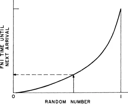
In this model passenger arrivals are considered
to be poisson with a known variable mean. A
passen-ger interarrival time is calculated for each station
w-J X zw L 0 FIGURE 3.2: 6:00AM RANDOM NUMBER PASSENGER INTERARRIVAL TIMES-POISSON PROCESS. 12:00 PM TIME OF DAY
FIGURE 3.1: DAILY VARIATION IN AVERAGE INTERARRIVAL TIME.
Specifically,
IA = FNl * FN2 (3.2)
where IA = Interarrival time
FNl = the selected interarrival time
FN2 = time of day variation multiplier
Arriving passengers queue up to await a dispatch
decision. Their arrival times and subsequent waiting
times are maintained by the program. Flight times,
fares and operating costs are assumed constant and
the same in either direction.
Aircraft may be pre-positioned where desired,
however the model in its present form does not possess
a capability to handle ferry flights from one station
to another.
3.2.2 Dispatch Strategy
At each station there are three separate rules
which are examined prior to a departure decision. Only
1. Capacity decision: This permits a departure when a full vehicle load is on hand.
2. Economic decision: This is the "marginal cost equals marginal revenue" concept. When the expected revenue from a further delay is less than the incremental delay penalty expected, then a departure is
initiated.
3. Coupled decision: This rule is intended to tie in the state at station 1 with the state at station 2. In this case the state
is a function of the number of passengers waiting and the disposition of aircraft. Waiting times per se do not enter into this decision.
Critera 1 is self-explanatory; criteria 2 is explained in Chapter 2. The third criteria, however is a pure heuristic. Basically it states that the more aircraft at, or on route to, station 1, the
TABLE 3. 2 - RUN SUMMARY TWO STATION MODEL - GPSS II
Run Number 1 2 3 4 5 6
Marginal
Decision Rule M M M M M M
(inactive)
Coupled No No No No yes Yes
DlyPnlyK1 1 1 1 11
Delay Penalty KD 2000 1000 1000 2~TIT 2000 2000
*
Time Horizon H 30 min 30 min f(T.O.D) f(T.O.D) f(T.O.D) f(T.O.D)
Run Time (min) 1000 1000 951 1000 1000 1000
Total Pax @ 1 256 241 240 230 230 230 @ 2 186 169 162 128 128 160 Total Return 1 797 -1725 3490 4415 4415 3451 2 -183 -2418 1160 1613 1613 1879 Total Delay Costs 1 142 159 2208 1476 1476 981 2 225 161 1057 1055 1055 1060 Flights From 1 9 12 4 3 3 4 2 7 10 4 2 2 3 Pax Left @ 1 11 26 6 37 37 37 2 1 18 9 59 59 27 Ave. Delay @ 1 35.7 27.2 84.5 91.5 91.5 75.2 2 47.9 30.8 69.5 113.6 113.6 91.5 Ave Load 27.6 18.6 50.3 71.5 71.5 56
must be available before an aircraft can be dispatched from 1. In Figure 2.11 any point outside the shaded area permits a departure.
This is a relatively simple attempt to link the decisions at the two stations. This rule may be
further refined by considering the expected passen-ger build-up at the other station during the sector
flight time, and some quantification of passenger waiting times.
3.2.3 Output Format
1. Schedule: The simulation generates a de-parture schedule showing
a) time of departure or timetable b) passenger load
c) net revenue for the flight
d) the number of aircraft remaining at the point of departure.
2. Queues: Statistics on queues at stations 1 and 2 are tabulated showing maximum- and average queue length, average waiting time, etc.
3. number of
Savex: The system maintains a count on a
parameters of interest, e.g.
a) Total accrued delay penalty at each station
b) Total fares collected at each station c) Total return per station
d) Number of arrivals and departures e) Number of aircraft flying, etc.
4. Tables: Statistics on passenger arrival
rates showing the means and standard deviation as well
as distributions are tabulated.
3.2.4 Discussion of Runs
Selected runs are tabulated in Table 3.2. The utility of the variable time horizon in the marginal
return dispatch criterion is seen in a comparison of
runs 1 and 4, and of runs 2 and 3. In 1and 2 a time horizon of 30 minutes is employed while in runs 3 and 4
the horizon is either 30 or 60 minutes depending on
the time of day. Note the substantial improvement
in total return realized in the latter case. The
reduction in the number of flights operated. Higher passenger average waiting times are reflected in the large delay penalties. However, these large penal-ties were more than offset by the cost savings re-sulting from higher load factors.
Runs 3 and 4 may be compared to determine the effect of changes in the weighting, or importance, assigned to the passenger waiting times. In run 3 the delay is weighted twice that of run 4. With the greater emphasis on passenger delays, flights depart earlier and with less passengers. Average waiting times decrease correspondingly while the return function suffers moderately.
Runs 5 and 6 were intended to evaluate the ef-fect of the coupling rule. In essence the coupling rule will tend to authorize a departure when a
higher percentage of the aircraft are at the station in question and when there are many passengers in the system, i.e., at both stations.
With a coupling parameter of 500 in Run 5, i.e.
where X = number of aircraft at or en route to the station
Y = number of passengers at the station
the rule was always inactive and performance was
identical to that of Run 4. In Run 6 a constant of
250 was tested in the rule. As might be expected better customer service resulted with a 1910%
reduc-tion in delay penalties. This is also seen in the
reduction in average passenger waiting times.
How-ever, net revenues suffered a decline of 11.6% due to an
extra two flights operated to r-ccomodate an additional
32 passengers. As they now stand, these rules are by no means in their most desirable form. Many more runs would be required and basic policy guidelines
of the airline would necessarily enter into consider-ation, especially with respect to the treatment of
CHAPTER 4
THE NINE STATION PROBLEM
The nine station model was built to depict a multi-station network problem with full interaction
between city-pairs. It was designed primarily to
evaluate the relative success of certain decision criteria and heuristics in realizing an improved level of operation, and to that end, to reflect the state of the system at any point in time.
As full interaction implies, both revenue and ferry flights are permitted from all stations to any of the other stations. Only non-stop service is considered, however, and there is no capability for multiple sector flights. This latter feature is a logical and important extension to the current problem.
4.1 Model Structure and Operation
An interval of time is taken to be 15 minutes. At each interval a transaction is created, representing some variable number of passengers wishing to travel
from point of origin A to destination B. This input transaction may be split into any number of similar transactions to permit simultaneous creation of passenger demands for a number of sectors in the system. For the system described here 16 such
transactions were introduced at each time interval. The origination-destination parameters (city-pairs) may be assigned values in a number of random or biased-random ways. Also the number of passengers
associated with a transaction may be determined in any desired way -- poisson, random, etc. In the
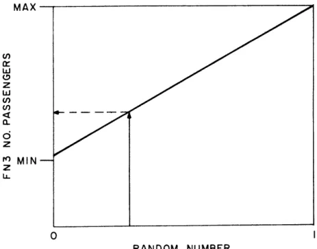
model constructed, a control loop selects a random number for each city-pair from an assumed distri-bution curve. This is taken to be the mean daily demand for that sector. This number, biased by a time of day variation parameter, (Figure 4.1) es-tablishes the number of arrivals in the given time period. Further a multiplier is included to
com-pensate for the number of time periods that are likely to be missed over the course of the day. The missed time periods occur since there are 72 city-pair
MAX w (D) z rO MIN z uL RANDOM NUMBER
FIGURE 4.2: DAILY TOTAL DEMAND DISTRIBUTION
6:00AM 12:00 PM
TIME OF DAY
FIGURE 4.1: DAILY DEMAND
period. For this case a multiplier of 72/16 or 5 would be in order. If warranted greater accuracy could be obtained by making a definite assignment for each city-pair combination at each time inter-val. The method used, however, reduces model size and introduces an additional element of randomness which is acceptable under such conditions of demand
uncertainty.
Arriving passengers queue up by city-pairs. In addition to the passenger state for each city-pair, a fare, operating cost and flight time structure for the associated sector is included. These are derived from the matrix shown in Figure 4.3. The 9 x 9 matrix is partitioned into nine 3 x 3 sub-matrices. All similarly labelled sub-matrices have common fare, operating cost and flight time structures determined by:
Sector fare per passenger = 10 x L ($) Sector operating cost = 250 x L ($) Sector flight time = 2 x L (15 min.
intervals)
TO
0
5 B -A
8 CB
9
ALL COMMON LABELS INDICATE
SIMILAR FARE, OPERATING COST, AND FLIGHT TIME BETWEEN CORRESPONDING
CITY-PAIRS
FIGURE 4.3: FARE/ COST/ FLIGHT TIME STRUCTURE
Initially the number of aircraft in the system is specified. Initial aircraft disposition may -be set deterministically or in a random fashion by a pre-position control loop. After simulation has commenced, the program routes the aircraft in ac-cordance with the dispatch and ferry decision and aircraft availability.
4.2 Dispatch Decision Rules
A number of dispatching criteria were tested on this model. The following demonstrated the most promising performance.
Dispatch when:
1. Aircraft capacity: A capacity load is available
2. Economic: The incremental passenger delay penalty to be experienced is greater than the marginal revenue ex-pected during the next time period. The time period is considered to be a variable function of the time of day.
3. Time limit: A parameter which is a function of the number of passen-gers waiting and the longest pas-senger waiting time exceeds a pre-set limit. This is intended to prevent extremely long delays when only a few passengers are on hand.
Of course in all cases an aircraft must be available at the station in question.
In addition to the decisions governing revenue flights, rules controlling the dispatch of ferry flights are also included. This rule is similar to criterion 3 above with the added condition that there must be a free aircraft somewhere in the sys-tem. In particular:
1. A parameter, which is a function of the number of passengers in the queue and the longest waiting time, exceeds a prespecified limit.
2. There are no aircraft at the station of origin.
3. There is at least one free aircrLaft on the ground in the system and as yet un-designated for service.
4. There have been no prior ferry calls which have not yet arrived.
5. There are no revenue flights on route to the station.
With these conditions satisfied, the program searches all stations starting at the nearest and will requisition the first free aircraft found. If there are passengers queued up for the particular sector to be ferried, the flight will be regarded as a revenue flight and dispatched immediately. Otherwise, the sector will be operated empty as a pure ferry. The total number of ferry flights flown and the associated costs are recorded at the completion of the run.
4.3 Output Format
For all revenue flights a departure schedule is generated showing:
1. Time of departure
2. Origin-destination code 3. Passenger load
4. Flight revenue (fares less costs)
Statistics are also tabulated on queues, reven-ue, and ferry flights, aircraft location, demand distributions, etc.
4.4 Discussion of Runs
The runs for this model were intended to evalu-ate the relative merits of various decision criteria and the sensitivity of other determinants operating
in the system. Consequently, the measurements are not of particular interest for their absolute values, but rather for the magnitude and direction of the de-viation effected by a controlled change somewhere in
the system.
Overall performance is measured by two parameters: 1. Total profit for the period (fares less
2. Average passenger queue lengths for the period of the run.
The first is a measure of the overall economic success from the airline's standpoint. The second
is a measure of the level of service provided to the customer.
In the interest of computer time economy, simu-lation runs were allowed to run for 7 hours, from 6:00 AM through the peak period of the morning and into the slack of the afternoon, until 1:30 PM.
These were considered representative for the purpose of this report, however, for more accurate comparisons, longer runs would be required, extending not only
through the full day but over several days. This is of particular importance in view of the random selec-tion techniques employed by the model.
A summary of some of the runs are tabulated in Table 4.1.
TABLE 4.1 SELECTED RUN SUMMARY
NINE STATION MODEL
58 59 63 68 72 74 75 76 77 78 79 80
(Low) (High (Med)
Passenger Demand L L H L L L L L M M M Delay Pen. K, _ 1 1 3 3 3 3 5 1/4 1/4 5 1 * rime Horizon H 3V 3V 3V 3V 3V 3V 3V 3V 3V 3V 3V 2 V Guarantee K 5 10 25 25 25 25 25 25 25 25 25 25 Run Duration 450 450 450 450 450 450 450 450 450 450 450 450 Demand Expect. 1/6 1/6 3/2 3/2 1/6 1/6 1 1/6 1/6 1/3 1/3 1/3 No. Aircraft 10 10 15 5 20 5 10 10 10 10 10 10 Net Revenue -7960 -5820 9220 9130 -4000 -3010 -4180 -4410 -3800 -1090 - 2330 -1520
No. Rev. Dep. 26 23 26 24 21 17 19 20 17 20 23 21
No. Ferries 1 1 0 0 0 3 0 0 0 0 1 1
Cost of Ferries 250 500 0 0 0 1500 0 0 0 0 250 250
No. Pax Carried 215 238 1146 963 297 260 237 239 225 414 433 422
No. Times Rev.Ferry 9 5 3 15 3 6 6 6 6 6 6 9
Criteria Capacity 0 0 11 2 0 0 0 0 0 0 1 0
Used Economic 6 12 6 5 15 10 12 14 9 10 13 8
Guarantee 12 7 7 3 4 2 2 1 3 5 4 5
Total Delay Cost - - - 14.431 3798 10.463 6357 10.621 688 455 14.238 3747
Ave. Load 8.3 10.3 41.1 40 14.1 15.3 12.5 11.9 13.2 20.7 18.8 20.1
Ave. No. Pax Waiting 5.2 5.0 55.8 62.4 6.4 7.15 4.9 4.8 5.6 10.3 10.1 10.5
4.4.1 Effect of the Delay Penalty
The assignment of values to the passenger waiting
times is believed to be an important factor in any
economic dispatching criterion. To determine just
how important and through what mechanism it operates,
several identical runs were made with only the
sub-jective delay penalty constant changed.
Runs were made at two levels of demand, the
results of which are presented in Figure 4.4. The
general trend for both demand levels is a
deteriora-tion in economic performance as the delay penalty is
increased. Notice that there exists a range in which
no change is experienced. The measure of passenger service, average queue length, runs contrary to the
economic trend and improves with increasing delay penalty.
Increasing the delay constant induces earlier
departures. However, in the range between K = 2 and
4, at least for the conditions of this case, the delay
-6000 - 5000
I-Bi -4000 3000 -- 2000
H
- 1000 LOW R DEMAND 0 0 0 (M/2) 0--2L
MEDIUM 0 _ _ R DEMAND (M) - ---0-0I~Q
II
_ .1 2 3 4DELAY PENALTY CONSTANT, KD
FIGURE 4.4: EFFECT OF DELAY PENALTY CONSTANT
ii
10.5
expected. Beyond 4, however, this is reversed, and
a flight is dispatched earlier. This later
precipi-tated a ferry flight which was not required for the
case of the lower delay constants. This higher penalty cost thus resulted in fewer passengers carried (by 5)
and one extra flight. For other fare/cost structures and passenger arrival rates, a different 'break-point'
would most probably exist.
If no passengers are expected over the time
horizon, the economic decision criterion would
auto-matically dictate a departure since the fare
incre-ment (=0) would always be less than the delay
increment. This may be detrimental and suggests the desirability of coupling this criterion with an
added requirement for minimum number of passengers.
This is especially significant in a low demand situ-ation when the probability of any passengers arriving
in the next time interval is very small.
Average loads in the low demand case range
from 12 to 13. In the higher demand case (twice
the lower) the average load varies between 20 and
conducted for an even higher demand case (ten times the lower). For this run, average loads were at about 54, up slightly over four times. With more efficient use of the aircraft implied by higher average loads, substantial improvements in gross or net revenues result. However, as seen, load factors do not automatically increase proportion-ately with customer demand. Perhaps a useful by-product of this model is in its ability to indicate reasonable aircraft capacities for a given fleet
size and demand expectation. With slight modifi-cation it may also be used to determine fleet size for given capacity aircraft.
Ferry flights can be a source of distortion in trends. When called, a ferry is drawn from available
aircraft in the system. If one is nearby, a cost of $250 is incurred, but if it is far away, as much as $750 surcharge must be paid for the same service. This ferry, being further away, also takes longer to arrive. Therefore, in addition to the extra cost, longer waiting times are suffered. Longer periods
of running the model are required to average out the
distortions from such effects.
4.4.2 Effect of the Time/Passenger Waiting Constraint
Aside from the economic and capacity criteria,
the third criterion in the decision rules, an upper
bound on the delay time, also plays a significant role. This criterion essentially places a limit or
threshold on the number of passengers waiting and the
time they have been waiting. The more passengers
waiting, the less waiting time required to trigger a
dispatch (or call for a ferry). Conversely, the
fewer the passengers, the longer the time they are required to wait before the criteria is satisfied.
That is, the longest waiting time (in 15 minute inter-vals) plus number of passengers waiting must be greater
than the threshold specified. Of course, this criterion may be overridden by the capacity and economic criteria.
Thresholds of 5, 10, 15, 20, and 25 were examined under
two levels of demand, one twice the other. All other
variables in the system were held constant. As seen
- 6000
r-MEDIUM DEMAND DELAY PENALTY CONSTANT, KD=I
Nb Nb /K 0 - 2000 k--000 5 10 15 20 2 PASSENGER/TIME THRESHOLD
FIGURE 4.5: EFFECT OF PASSENGER GUARANTEES
-67--5000 ---, 13 -H 12 - -4000 z Ld -3000 .00 Xs- ..- - - -: z Li Li Li -H 9