Dynamic optimization of a district cooling distribution network

HAL Id: tel-03066242

https://tel.archives-ouvertes.fr/tel-03066242

Submitted on 15 Dec 2020

HAL is a multi-disciplinary open access archive for the deposit and dissemination of sci-entific research documents, whether they are pub-lished or not. The documents may come from teaching and research institutions in France or abroad, or from public or private research centers.

L’archive ouverte pluridisciplinaire HAL, est destinée au dépôt et à la diffusion de documents scientifiques de niveau recherche, publiés ou non, émanant des établissements d’enseignement et de recherche français ou étrangers, des laboratoires publics ou privés.

Dynamic optimization of a district cooling distribution

network

Arley Fernando Nova Rincón

To cite this version:

Arley Fernando Nova Rincón. Dynamic optimization of a district cooling distribution network. Chem-ical and Process Engineering. Université de Pau et des Pays de l’Adour, 2019. English. �NNT : 2019PAUU3020�. �tel-03066242�

1

THÈSE

UNIVERSITE DE PAU ET DES PAYS DE L’ADOUR

École doctorale des sciences exactes et leurs applications (ED211)

Soutenance prévue le 4 Octobre 2019

par Arley NOVA RINCÓN

pour obtenir le grade de docteur

de l’Université de Pau et des Pays de l’Adour

Spécialité : Énergétique

Optimisation dynamique d’un système de distribution

de froid à l’échelle urbaine

-Dynamic optimization of a district cooling distribution network-

MEMBRES DU JURY

RAPPORTEURS

• Galo Antonio CARRILLO LE ROUX Professeur / Université de São Paulo(USP) – Brésil • Jorge Mario GÓMEZ RAMÍREZ Professeur Associé / Université des Andes – Colombie

EXAMINATEURS

• Pascal FLOQUET Professeur des Universités / ENSIACET Toulouse

• Sabine SOCHARD Maître de Conférences / Université de Pau et des Pays de l’Adour

DIRECTEURS

• Jean-Michel RENEAUME Professeur des Universités / Université de Pau et des Pays de l’Adour

• Sylvain SERRA Maître de Conférences / Université de Pau et des Pays de l’Adour

ii

Acknowledgements

Firstly, I would like to express my sincere gratitude to my advisors Dr Sabine Sochard (M.C), Dr Sylvain Serra (M.C) and Prof. Jean Michel Reneaume for the continuous support during these three years of research work, also for their patience, and motivation. I would like to extend a special acknowledgement to Sabine, for her close guidance in the development of this manuscript as well as for her interest in my full understanding of the implemented methods.

Besides my advisors, I would like to thank the rest of my thesis committee: Prof. Galo Carrillo Leroux, Prof. Jorge Mario Gómez Ramírez and Dr Pascal Floquet, for their insightful comments and questions which allowed me to widen the scope my research work. Particularly, I am grateful to Pr. Gómez for enlightening me the first glance of the world of research in process optimization at Universidad de Los Andes.

I thank my colleagues (PhD candidates) and professors at the LaTEP, as well as all the staff at the ENSGTI, for their always welcoming attitude and their important role in the improvement of my linguistic skills in the French language.

Moving to more personal expressions of gratitude, I thank the families Bedoya-Velez and Martinez-Lopez, for becoming my family of adoption here in France. Thanks for all the good moments, mainly for all the mountain bike journeys with Daniel, Pablo and Angel. The “escape plans” you proposed were an authentical relief in the stressful moments.

Here, I would like to thank my family: my parents and my sister for supporting me spiritually from the distance throughout these three years. This thesis is the result not only my effort but also of all the values I learned at home, the discipline, the persistence and the conscientious work.

Finally, and with the most intense feelings of admiration and love, I express all my gratitude to my wife Natalia, for accepting the challenge of taking this road by my side, three years ago. Thank you for being my confidant, and my counsellor in the most complicated and stressful moments during this process. Most of my motivations came from her incomparable support.

More valuable than the work I present in this manuscript, are all the things that I have learned, both intellectually and personally, in this remarkable life experience of doing a PhD.

iv

Abstract

Dynamic optimization of a district cooling distribution network

Arley NOVA-RINCÓN

Supervisors: Jean-Michel RENEAUME, Sylvain SERRA Laboratoire de Thermique, Energétique et Procédés (LaTEP)

Due to the increasing demand for cooling worldwide and the need for reliable and energy-efficient alternatives to provide it, the analysis of district cooling (DC) networks has become a focus of interest in recent years. Currently, most of the developments in the field of numerical simulation and optimization of these systems have been done by implementing steady-state models. Considering this, in the present work we proposed a methodology based on mathematical programming for the dynamic simulation and optimization of the distribution system in district cooling networks.

The dynamic model includes a partial differential equation to describe the variation of the temperature in the pipes, and heat and mass balances in the users and in the interconnecting nodes of the network. This arrangement is known as a partial differential algebraic equation (PDAE) problem. We detail the implementation of 2D- Orthogonal Collocation on Finite Elements (OCFE) for the discretization of the dynamic problem. Then the previously discretized model is added to the optimization constraint set, according to the simultaneous (equation-oriented) solution strategy. The optimization variables (decision variables) include the spatial and temporal profiles of the temperatures and temporal profiles of the mass flows of the system. Additional optimization variables (pipe diameters…) are progressively introduced. We apply this methodology for the analysis of an operational and a cost objective function in a medium size cooling system, serving 20 consumers grouped in five different categories with fluctuating cooling demands subject to variable external conditions. The first objective function considers that in DC networks, the temperature of the cooling utility returning to the production site must be close to the design temperature of the installed technology to ensure proper efficiency and avoid the technical issue known as low ΔT syndrome. Then, still ensuring this condition, the second objective function aims to minimize a cost function (production and pumping costs) including the diameter of the pipes as decision variables. The methodology allowed the computation of the optimal mass flow profiles to operate the system under the desired conditions and the estimation of the pipe diameters of the distribution network for two different costs of production. For the two objective functions, the dynamic simulation and optimization were performed using insulated and non-insulated piping.

The proposed methodology exhibits low CPU cost that demonstrates its potential use for the development of applications for the operation and forecasting of distributed systems.

v

Résumé

Optimisation dynamique d’un système de distribution de froid à

l’échelle urbaine

Arley NOVA-RINCÓN

Directeurs: Jean-Michel RENEAUME, Sylvain SERRA

UNIV PAU & PAYS ADOUR / E2S UPPA, Laboratoire de Thermique, Énergétique et Procédés-IPRA

L’utilisation de froid (industriel et climatisation) dans le monde ne cesse d’augmenter et les prévisions annoncent un accroissement continu de la demande de froid dans les années à venir. De ce fait, la recherche d’un moyen fiable et performant permettant la fourniture de froid est plus que jamais d’actualité. Dans ce contexte, les réseaux de froid urbains sont de plus en plus étudiés. Actuellement, la plupart des études portant sur la simulation numérique ou l’optimisation de ces systèmes ont été mises en œuvre en régime stationnaire. Compte tenu de cela, le présent manuscrit propose une méthodologie de résolution mathématique pour la simulation et l’optimisation dynamiques d’un réseau de froid urbain.

Le modèle dynamique inclut les équations différentielles permettant de représenter les variations de température dans les canalisations, ainsi que les bilans de masse et d’énergie aux nœuds du réseau et dans les échangeurs thermiques alimentant les consommateurs. Le modèle ainsi construit est un système d’équations aux dérivées partielles et algébriques. Nous détaillons la méthode de double collocation orthogonale sur éléments finis permettant de discrétiser ces équations afin d’obtenir un système comprenant uniquement des équations algébriques. Le modèle ainsi discrétisé est alors ajouté aux contraintes du problème d’optimisation à résoudre, conformément à la stratégie de résolution orientée équations. Les variables d’optimisation (de décision) sont les profils spatiaux et temporels de température et les profils temporels de débit dans tout le système. D’autres variables d’optimisation, tels que les diamètres des canalisations, sont ajoutées par la suite. Cette méthodologie d’optimisation dynamique est résolue pour deux fonctions objectif différentes (exploitation et économique) appliquées à un cas test, inspiré de la littérature, comprenant 20 consommateurs représentant 5 catégories de bâtiments différents ayant des demandes temporelles de froid variables. Tout ceci est soumis aux variations de température extérieure pour différentes localisations.

La première fonction objective a pour but de maintenir la température de retour dans l’unité de production de froid proche de la température considérée pour le dimensionnement de cette unité afin d’assurer un fonctionnement efficace et d’éviter un problème bien connu dans les réseaux de froid appelé « low ΔT syndrome ».

Ensuite, en garantissant toujours un tel fonctionnement, la seconde fonction objective a pour but de minimiser une fonction coût incluant les coûts de production de froid et de pompage dans le réseau

vi

en considérant les diamètres comme variables d’optimisation. Une procédure particulière, enchainement de simulations stationnaires puis dynamiques, est proposée afin d’obtenir une initialisation permettant la convergence vers un optimum de confiance du problème d’optimisation dynamique. Cette méthodologie a permis d’obtenir les profils temporels optimaux des variables de contrôle du système dans les conditions d’utilisation désirées ainsi que les diamètres de l’ensemble du réseau pour deux coûts représentant différents types de technologies de production de froid. Les simulations et optimisations dynamiques (pour les deux fonctions objectif) ont été réalisées pour des tuyaux isolés et pour des tuyaux non isolés.

La méthodologie mise en place présente un temps de résolution faible sur un ordinateur portable classique ce qui démontre son potentiel d’utilisation pour le développement d’application de contrôle et de prédiction de ce type de système.

Keywords: Réseau de froid, optimisation dynamique, Double collocation orthogonale sur éléments finis

Contents

INTRODUCTION……….1

Chapter 1. District Cooling Systems ... 12

1.1 District Energy Systems ... 14

1.2 District Cooling Systems ... 16

1.2.1 Generalities of district cooling... 17

1.2.2 Challenges on research in District Cooling ... 24

1.3 Dynamic modelling and simulation in DHC ... 25

1.4 Optimization approaches ... 28

1.5 Basics on Dynamic optimization ... 34

1.5.1 Basic Example ... 34

1.5.2 Formulation of a dynamic optimization problem ... 36

1.6 Collocation Methods ... 39

1.7 Thesis objectives ... 41

Chapter 2. Case study and mathematical model ... 44

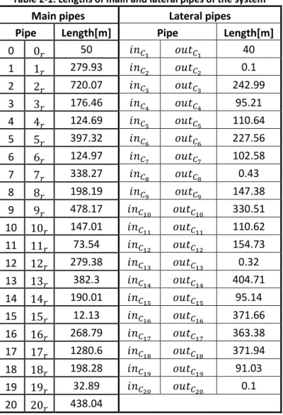
2.1 Case Study System ... 46

2.1.1 System’s configuration ... 46

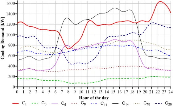
2.1.2 Consumers and their cooling demands ... 47

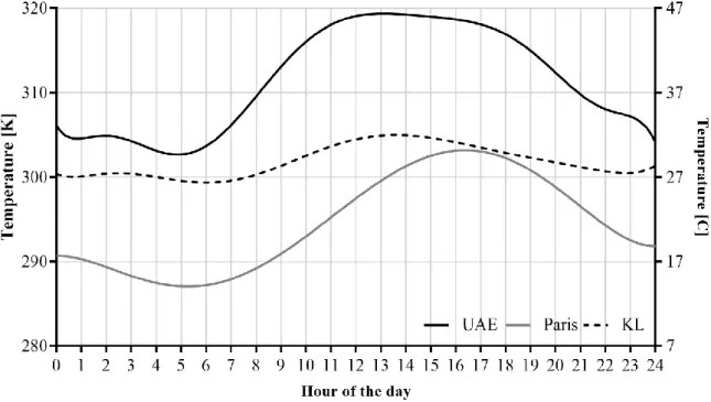
2.1.3 Soils and climate zones ... 49

2.2 Mathematical model ... 51

2.2.1 Heat balance in the pipes ... 51

2.2.2 Heat balances in the nodes ... 51

2.2.3 Mass Balances in the nodes ... 52

2.2.4 Degrees of freedom and flow policy ... 53

2.2.5 Flow velocities ... 55

2.3 Discretization strategy and mathematical model ... 57

viii

2.3.2 The collocation matrix ... 58

2.3.3 Implementation of 2D OCFE ... 61

2.3.4 The discretized model ... 64

Chapter 3. Dynamic simulation Analysis ... 68

3.1 Initialization and solution strategy ... 70

3.2 Simulation Results ... 73

3.2.1 Pipe diameters ... 73

3.2.2 Steady-state simulation ... 76

3.2.3 Dynamic simulation analysis ... 80

3.3 Conclusions of the simulation analysis ... 84

Chapter 4. Dynamic Optimization Analysis ... 86

4.1 Objective function: Avoiding low ΔT syndrome ... 88

4.1.1 Dynamic optimization under constant flow policy ... 90

4.1.2 Dynamic optimization using variable mass flows ... 93

4.2 Objective function: Operational cost ... 98

4.2.1 Formulation ... 98

4.2.2 Initialization strategy ... 103

4.2.3 Results and discussion ... 104

4.3 Conclusions of the Dynamic Optimization Analysis ... 112

CONCLUSIONS AND PERSPECTIVES………111

ix

List of figures

Figure 1-1. Energy sources for heating and cooling, based on data in [4] ... 14

Figure 1-2. General scheme for a DHC system ... 15

Figure 1-3 Energy use in the European market in 2015, Based on ref [15] ... 16

Figure 1-4. Flexibility and integration of technologies in DCS... 19

Figure 1-5. Mapping of district cooling in Europe in 2006 (biggest per country have a star) as presented in ref.[30] ... 20

Figure 1-6. Specific cooling demands by country, based on data in ref[32] ... 21

Figure 1-7. Indicative mapping of DHS (left) and DCS (right) in France[33] ... 22

Figure 1-8. Map of the Parisian Cooling Network[35] ... 23

Figure 1-9. Representation of a buried pipe ... 26

Figure 1-10. Comparison of research in Optimization of district heating and district cooling systems 28 Figure 1-11. Illustrative example of dynamic optimization ... 35

Figure 1-12. Feasible trajectories (a) and Optimal trajectory for the moving block problem ... 35

Figure 1-13. Optimal force trajectory for minimum absolute work ... 36

Figure 1-14: Solution strategies for dynamic optimization problems ... 37

Figure 2-1. Representation of the cooling network ... 47

Figure 2-2. Demand for different kind of buildings ... 48

Figure 2-3. Cooling demands of major consumers per building category ... 49

Figure 2-4. Summer Temperature profiles in the studied climate zones ... 50

Figure 2-5. Constant flow policy diagram ... 54

Figure 2-6. Spatial representation of 1D-OCFE ... 57

Figure 2-7. Representation of the temperature discretization (one element per domain)... 62

Figure 2-8. Associated equations for the solution of the discretized PDE ... 66

Figure 3-1. Methodology for the initialization and solution of the dynamic optimization problem .... 71

Figure 3-2. Total demand and localization of 𝑡𝑚𝑎𝑥 to define demands for steady-state simulation .. 72

Figure 3-3.Variation of the total thermal resistance ... 75

Figure 3-4. Comparison of spatial distribution of temperature for different number of points ... 76

Figure 3-5. Spatial distribution of temperature in the outward path of the network ... 78

Figure 3-6. Spatial distribution of temperature in the return path of the network... 80

Figure 3-7. Return temperature profile for different arrangements of finite elements and collocation points ... 81 Figure 3-8. Outlet temperature in consumers 1 and 11 for constant flow policy under KL conditions 82

x

Figure 3-9. Outlet temperature in consumers 13 and 20 for constant flow policy under KL conditions

... 83

Figure 3-10. Return temperature under constant flow policy for KL conditions ... 84

Figure 4-1. Dynamic flow policy diagram ... 89

Figure 4-2. Return temperature profiles under for DO-1 ... 91

Figure 4-3. Outlet temperature profiles in consumers 1 and 11 for DO-1 ... 92

Figure 4-4. Inlet Temperature profile for selected consumers under constant flow... 92

Figure 4-5. Return Temperatures for consumers C4 and C16 ... 93

Figure 4-6. Temperature profiles for dynamic flow policy ... 94

Figure 4-7. Velocity profiles of the pipes trespassing upper bounds ... 95

Figure 4-8. Optimal production and inlet mass flow for chosen consumers ... 95

Figure 4-9. Production site power comparison ... 97

Figure 4-10. Definition of the maximum velocity per pipe diameter size ... 99

Figure 4-11. Variation of the pipe wall thickness respect to the internal diameter ... 100

Figure 4-12: Variation of the insulation thickness as function of the internal diameter ... 100

Figure 4-13. Procedure for the solution of the cost optimization ... 103

Figure 4-14. Dynamic resistance profile in selected pipes ... 105

Figure 4-15. Dynamic thermal resistance and the influence of mass flow for non-insulated pipe 13 105 Figure 4-16. Dynamic thermal resistance and the influence of mass flow for insulated pipe 13 ... 106

Figure 4-17. Total pressure drops per branch ... 106

Figure 4-18. Pressure drops comparison between DO2 and DO3 using 𝐶𝑐𝑜𝑙𝑑1 ... 108

Figure 4-19. Optimal diameters for DO3 using 𝐶𝑐𝑜𝑙𝑑1 ... 108

Figure 4-20. Return temperature profile for 𝐶𝑐𝑜𝑙𝑑1 ... 109

Figure 4-21. Pressure drops for DO3 using 𝐶𝑐𝑜𝑙𝑑2 ... 110

Figure 4-22. Optimal diameters for DO3 using 𝐶𝑐𝑜𝑙𝑑2 ... 110

1

List of Tables

Table 1-1. Distribution of heating and cooling networks in France ... 22

Table 1-2. Classification of works on Optimization of DHC ... 29

Table 2-1. Lengths of main and lateral pipes of the system ... 46

Table 2-2. Consumer’s peak cooling demands ... 48

Table 2-3. Soil thermal conductivities ... 49

Table 2-4. Analysis of degrees of freedom of the system ... 53

Table 2-5. Maximum allowable speeds in pipes ... 55

Table 3-1. Pipe diameters for the DCS ... 73

Table 3-2. External temperature and results for steady-state simulations ... 77

Table 3-3. Convective heat transfer per unit length at the production sites ... 78

Table 3-4. Mass flow in main outward pipes for steady-state analysis ... 79

Table 4-1. Comparison of production and inlet clients mass flows ... 90

Table 4-2. Total chilled water production for the studied pumping methods ... 96

Table 4-3. Evaluation of the Cost of operation for DO 2.1 ... 107

Table 4-4. Value of the objective function elements for DO3... 107

Table 4-5. Percentage differences for the cost DO3 respect to DO2.1 ... 107

2

NOMENCLATURE

Symbols

𝐶𝑐𝑜𝑙𝑑 Cost of producing cold utility €/kWh

𝐶𝑒𝑙𝑒𝑐 Cost of electricity €/kWh

𝐶𝑝 Specific Heat Capacity, J/(kg.K)

𝐷𝑖 Internal diameter of pipes m

𝐿 Pipe length m

𝐿𝑓 Length of spatial finite element

𝑚̇ Mass flow rate kg/s

𝑁𝑥 Spatial collocation matrix

𝑁𝑥 Temporal collocation matrix

𝑃𝑤 Power in the production site kW

𝑃𝑤𝑝𝑢𝑚𝑝 Electrical energy demanded by the pump kWh

𝑄 Cooling Demand kW

𝑟𝑎 Internal radius of the pipe m

𝑟𝑏 External radius of the pipe m

𝑟𝑐 Radius including insulation layer m

𝑟𝑑 Radius including casing layer m

𝑅′ Total thermal resistance m.K/W

𝑡 Time s

𝑇 Temperature K

𝑣 velocity m/s

𝑊𝑝𝑢𝑚𝑝 Mechanical work of the pump kJ

Greek symbols

∆𝑃 Pressure drops kPa

∆𝑇 Temperature difference K

∆𝑡𝑒 Size of temporal finite element

𝜂𝑝𝑢𝑚𝑝 Total efficiency of the pump

𝜆 Coefficient of friction

𝜌 Density Kg/m3

𝜉 Normalized spatial variable 𝜏 Normalized time variable 𝜃 Steady-state temperature

3 Sets and index

𝐶𝑝 Set of consumers

𝐷𝑡_𝑖 Linear transformation for time derivative

𝐷𝑥𝑗 Linear transformation for space derivative

𝑒 Index for time elements 𝑓 Index for distance elements

𝑖 Index for time collocation points in time 𝑗 Index for distance collocation points 𝑘 Index of pipes

𝑝 Sub-index for main pipes

𝑖𝑛𝐶𝑝 Sub-index for pipes entering to clients

𝑜𝑢𝑡𝐶𝑝 Sub-index for pipes leaving clients

𝑟 Return pipe

𝑠 Soil

4

INTRODUCTION (ENG)

Cooling is used for diverse purposes in different sectors, from industrial refrigeration to guarantee safe food storage, transport, commercial to domestic refrigeration and air-conditioning. It is also important for the supply of medicines, cooling data centres, production of chemicals, plastics, metallurgic processes, and many other sectors and usages. This diversity of applications and the growing demand for cooling services, that only in the building sector has doubled since 2000, due to the combination of warmer temperatures and increased activity caused by population and economic growth, demand efficient and affordable solutions. Here, district cooling systems (DCS) arise as a potential technology to supply these needs with both lower cost and environmental benefits. District cooling networks together with district heating networks represent a category of distribution of utilities known as district energy systems. Particularly, DCS supply chilled water produced in a central (or multiple) plant(s) to buildings and industrial sites through a network of underground pipes. The chilled water can be produced using the same technologies than in air conditioning systems (compression refrigeration cycles), but generally at a much larger scale. More sustainable technologies include the use of natural sources of cold (sea, rivers, deep lakes and groundwater) or heat (residual heat from industry, geothermal or even solar thermal sources) to as utility for refrigeration cycles.

Considering the advantages of DCS in terms of energy efficiency and reduction of emissions, the European Union has been supporting the development of many projects led by industrial-academic consortiums aiming to improve system planning, control and management of district cooling systems, as well as their development and implementation using low and zero carbon-emitting sources. Mathematical programming has supported these advances, implementing complex models and innovative methods, including optimization techniques to obtain more accurate and representative results. The literature reports numerous works at the design stage, concerning the optimization of the cost of investment. These include the network topology, optimizing the sizing (pipe diameter, heat exchanger area) and operation (temperature, mass flow rates) parameters in order to minimize the investment cost while respecting a set of constraints (demands of consumers, temperature level). These works have led to optimum results corresponding to the nominal working conditions of the network assuming a steady-state operation. Nevertheless, the incursion of renewables to produce energy and the diversity of demands of the potential new consumers to be interconnected require the development of tools based on fully dynamic models. These dynamic-based tools will allow improving the operation, design, control and forecasting of the current and future systems, considering variations in the levels of demand of the consumers, in the environmental conditions of the location where the systems are installed, and in the production when renewable sources are used, leading to the use and

5

management of storage systems. Today, the development of applications for the analysis and optimization of district cooling systems based on dynamic models is scarce. Then, this is an important area that needs to be studied for the development of tools that respond to the current challenges in the operation and design of these systems.

Considering this, the objective of this thesis is to develop a methodology for the dynamic optimization of the distribution system of a district cooling network. This will allow computing the optimal temporal profiles of the operation parameters of the distribution system, considering also variations in the ambient temperature. The implemented methodology is illustrated thanks to a medium size distribution system serving 20 users with specific variations and levels of demand. The work of research for the development of this methodology is presented in the present manuscript that is divided into four chapters.

Chapter one presents a literature review that includes the generalities of district cooling systems and their development in Europe and in France. Then, the chapter introduces the challenges that the development of these systems imposes, including the importance of developing optimization tools based on dynamic modelling. The review also details previous works on the optimization of distributed energy systems. Then we introduce the generalities of dynamic optimization, including the methods that can be implemented for the solution of this kind of problems. Based on the literature findings, we introduce the method we chose for the discretization of the dynamic problems (orthogonal collocation on finite elements) to finish with the objectives of this thesis.

Chapter two details the topology, consumers’ cooling demands and the external conditions for the proposed case study. Using this illustrative example, the chapter details the mathematical model of the system, including an analysis of the degrees of freedom that will be considered for the optimizations. To conclude, we present the implementation of the discretization strategy for the solution of the dynamic problem.

Considering the discretized model, Chapter three introduces the methodology for the proper initialization of the dynamic optimization problems. The methodology is based on the successive solutions of steady-state simulations to initialize a dynamic simulation problem, whose results will be used as initialization for the dynamic optimization analyses. The chapter details the results of the intermediate simulations that include the definition of diameters and thermal resistances in the pipes, the distribution of temperatures along with the distribution network, and the response of the network

6

to the variations in demand and external conditions for a constant flow policy. The analysis is made for insulated and non-insulated pipes.

Finally, Chapter four presents the two proposed objective functions and their corresponding results. The first one aims to compute the optimal mass flow profiles that guarantee a constant temperature on the pipes leaving the consumers to avoid a common technical issue in district cooling known as “low T syndrome”. The second objective aims to find the optimal pipe diameters that minimize the value of an operational cost that considers the cost of producing the cold utility and the electrical power demanded by a pump sending the chilled water to the network. The two objective functions are evaluated using both insulated and non-insulated pipes. The consistency of the results presented in Chapters three and four and the reported computational times highlight the robustness of both, the chosen discretization strategy and the proposed methodology of solution.

INTRODUCTION (FR)

De nombreux secteurs, allant de la réfrigération industrielle, pour garantir la conservation des aliments, à la climatisation des commerces, transports et habitations, nécessitent du froid. Les besoins en refroidissement sont également importants dans le secteur médical, dans les centres de données, dans certains procédés des industries chimiques, plastiques ou métallurgiques, et dans bien d’autres secteurs. Cette diversité d’applications et la demande croissante en froid, qui, rien que dans le secteur du bâtiment, a doublé depuis 2000 à cause du réchauffement climatique et de la croissance économique, implique la mise au point de solutions réalistes et efficaces. Dans ce contexte, les réseaux de froid apparaissent comme une solution capable de fournir ces besoins à des coûts relativement faibles avec, qui plus est, un bénéfice environnemental. Les réseaux de froid ainsi que les réseaux de chaleur constituent des systèmes énergétiques centralisés (de quartier). En particulier, les réseaux de froid fournissent de l’eau réfrigérée, produite dans une ou plusieurs unités de production, à différents bâtiments ou sites industriels par le biais d’un réseau de canalisations enterrées. L’eau réfrigérée peut être produite par le même type de technologie que pour les systèmes de climatisation (cycles frigorifiques à compression), mais à plus grande échelle. Cependant, on peut utiliser des technologies économiquement et écologiquement plus durables, telles que l’utilisation de sources froides naturelles (mer, eaux fluviales ou souterraines ou lacs profonds) ou de sources chaudes (chaleur fatale industrielle, géothermie ou chaleur solaire) alimentant des cycles frigorifiques à absorption par exemple.

Consciente des avantages des réseaux de froid tant sur le plan de l’efficacité énergétique que de la réduction d’émissions de gaz à effet de serre, l’Union Européenne soutient depuis plusieurs années le développement de projets portés par des consortiums constitués d’académiques et d’industriels, dont le but est d’améliorer la gestion (planification), la conduite et le contrôle des réseaux de froid, ainsi que leur développement et leur mise en œuvre avec des sources bas carbone. Dans le but d’obtenir des résultats précis et représentatifs, la programmation mathématique a permis la mise en œuvre de modèles complexes et de méthodes innovantes incluant des techniques d’optimisation. De nombreux articles présents dans la littérature font état de travaux concernant l’optimisation des coûts d’investissement à l’étape de conception. Il s’agit de calculer la topologie du réseau, le dimensionnement (diamètre des conduites, aires d’échange) et les variables de fonctionnement du réseau (températures, débits) qui minimisent le coût d’investissement tout en respectant un ensemble de contraintes (niveau de température, satisfaction des besoins des consommateurs). Ces travaux ont généralement fourni les points de fonctionnement nominaux des réseaux considérés, en faisant l’hypothèse d’un régime permanent. Cependant l’utilisation d’énergie renouvelable pour produire le

9

froid ainsi que la diversité des besoins des clients rendent nécessaires le développement d’outils basés sur des modèles dynamiques. Ces derniers permettront en effet d’améliorer la conduite, le dimensionnement, le contrôle et la gestion (planification) des systèmes, nouveaux ou déjà installés, en prenant en compte les variations de demande des différents consommateurs, les variations des conditions climatiques extérieures à la localisation où ces systèmes sont installées et les variations dans la production (cas de sources renouvelables – Solaire…) conduisant à l’utilisation et à la gestion de moyens de stockage. Actuellement le développement d’applications basées sur des modèles dynamiques pour l’analyse et l’optimisation de réseaux de froid est rare. Il y a donc un besoin urgent d’études portant sur le développement d’outils capables de répondre aux défis actuels que constituent la conception et la conduite de ces systèmes.

Dans cette optique, l’objectif de cette thèse est de développer une méthodologie pour l’optimisation dynamique du système de distribution d’un réseau de froid, qui permettra d’obtenir les profils temporels des paramètres de fonctionnement de ce système en prenant en compte les variations de la température ambiante. Cette méthodologie sera illustrée par un exemple de taille moyenne avec 20 consommateurs connectés, chacun avec son profil temporel de demande. Le travail de recherche mené pour le développement de cette méthodologie est présenté dans ce manuscrit de thèse divisé en quatre chapitres.

Le chapitre un présente une revue bibliographique commençant par les généralités sur les réseaux de froid et leurs implantations en Europe et en France. Ensuite, ce chapitre introduit les défis que le développement de tels systèmes impose, parmi lesquels le développement d’outil d’optimisation basés sur des modèles dynamiques. La revue bibliographique détaille alors les travaux ayant porté sur l’optimisation de ces systèmes énergétiques de distribution puis introduit les généralités concernant l’optimisation dynamique ainsi que les méthodes mises en œuvre pour résoudre ce type de problème. Sur la base des résultats de la littérature, nous introduisons la méthode que nous avons choisie pour la discrétisation des problèmes dynamiques (collocation orthogonale sur éléments finis) puis ce chapitre se termine avec la présentation des objectifs de la thèse.

Le chapitre deux détaille, pour le cas étudié, la topologie, les profils de demande des consommateurs et des profils de température extérieure suivant la localisation du réseau. A travers cet exemple, ce chapitre présente le modèle mathématique représentant la physique du réseau et une analyse de degré de liberté qui sera utile pour les optimisations. Ce chapitre se termine par la présentation de la mise en œuvre de la technique de discrétisation utilisée pour résoudre le système.

Le chapitre trois introduit la méthodologie pour initialiser correctement les problèmes d’optimisation dynamiques mettant en œuvre le modèle précédemment discrétisé. La méthode utilisée est basée sur

10

des résolutions successives de simulations quasi-statiques pour initialiser le problème de simulation dynamique dont les résultats seront utilisés pour initialiser les optimisations dynamiques. Ce chapitre détaille les résultats de ces simulations intermédiaires incluant, pour une politique de débit constant, la définition des diamètres et des résistances thermiques des canalisations, la distribution des températures le long des canalisations du réseau, et la réponse du réseau aux profils de demande et de température extérieure. Cette analyse est faite pour des tuyaux isolés et non-isolés.

Le chapitre quatre présente les résultats d’optimisations dynamiques considérant deux types de fonctions objectif. La première permet de calculer les profils optimaux des débits permettant de respecter une température constante dans les canalisations quittant chaque consommateur, ceci afin d’éviter un problème technique classique dans les réseaux de froid appelé syndrome du faible T (low T syndrom). La seconde fonction objective cherche, en plus, à obtenir les diamètres optimaux des canalisations qui minimisent, cette fois, un coût opérationnel calculé sur la base d’un coût de production de l’utilité froide et du coût de l’énergie électrique nécessaire au pompage de l’eau froide à travers le réseau. Les deux fonctions objectives sont calculées pour des canalisations isolées et non-isolées.

Finalement, la cohérence des résultats présentés dans les chapitres trois et quatre et les temps calcul annoncés mettent en évidence la robustesse de la stratégie de discrétisation choisie et de la méthode de résolution proposée.

12

Chapter 1.

District Cooling Systems

As presented in the introduction of this work, the first chapter details the generalities and challenges in the development of district cooling systems. Based on these challenges, we introduce the objectives of this work and the tools and methods we propose to accomplish them.

Section 1 introduces the concept of district energy systems. From this, section 2 presents the generalities of district cooling systems and their development in the European and French markets. This section finishes presenting the current challenges in the research and development in this system with a focus on numerical applications. Following this, Section 3 presents a literature review of some approximations for the dynamic modelling of the district system. Then section 4 presents and categorize the applications in the optimization of district systems highlighting the lack of contributions based on dynamic models. Considering this, section 5 presents the generalities of dynamic optimization, including the formulation and the diversity of methods for their solution pointing out the advantages of the formulation based on collocation methods introduced then in section 6. Finally, section7 presents the objectives of the present work.

13

Chapter contents

1.1 District Energy Systems ... 14 1.2 District Cooling Systems ... 16 1.2.1 Generalities of district cooling... 17 1.2.2 Challenges on research in District Cooling ... 24 1.3 Dynamic modelling and simulation in DHC ... 25 1.4 Optimization approaches ... 28 1.5 Basics on Dynamic optimization ... 34 1.5.1 Basic Example ... 34 1.5.2 Formulation of a dynamic optimization problem ... 36 1.6 Collocation Methods ... 39 1.7 Thesis objectives………..41

14

1.1 District Energy Systems

According to 2017 data, heating and cooling account for half of the energy consumption in the European Union [1], [2]. From which, 45% is used in the residential sector, 36% in industry and 18% in services [3]. Furthermore, most of the fuel used by for heating and cooling still comes from non-renewables (75% as estimated by the European Commission [4] and detailed in Figure 1-1 ), representing a major source of CO2 emissions that need to be urgently mitigated [3], [5], [6].

Figure 1-1. Energy sources for heating and cooling, based on data in [4]

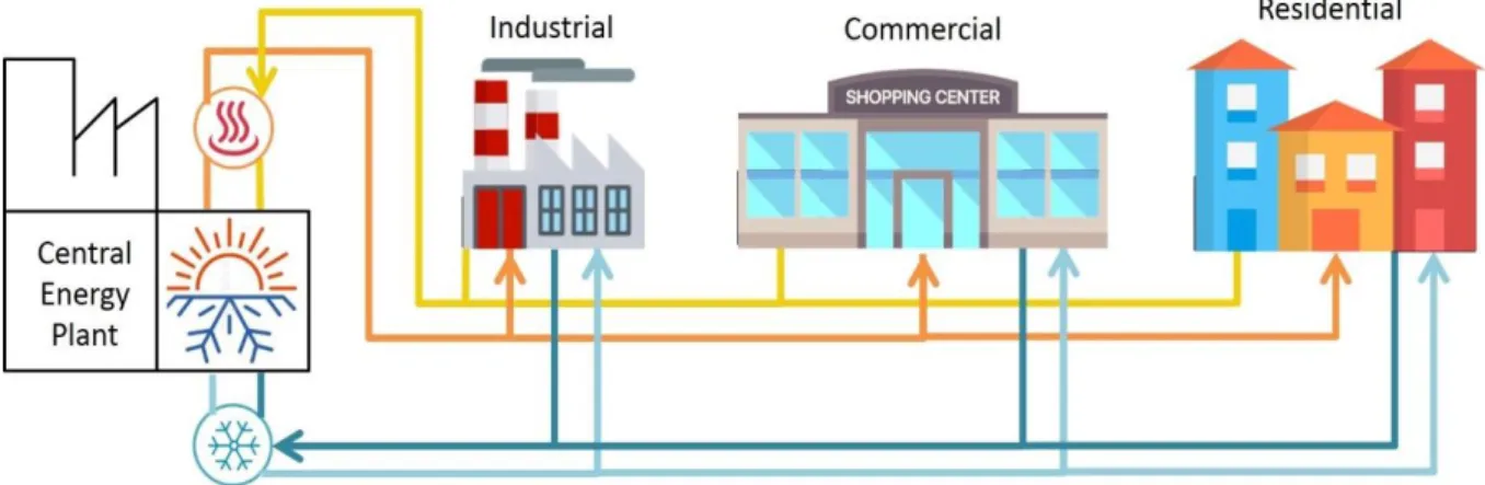
Being aware of this, district energy systems arise as an interesting alternative to mitigate the environmental impact caused by these emissions [1], [2], [7]. Indeed district energy systems, known also as District Heating and Cooling systems (DHC) [8], consist of a network of underground insulated pipes that pump hot or cold utility from a central energy plant and route it to multiple buildings in a district, neighbourhood or city [9]. The utility gives or takes heat from the user, according to the case, and then recirculates back to the central plant through a close-loop return line as shown in Figure 1-2. As stated by Lake et al. [10] and Rezaie and Rosen [11] in their reviews, these systems compared with individual heating and cooling equipment, have higher efficiency, are more economically attractive for high demand buildings, reduce fuel consumption, improve community energy management and allow a better control of emissions.

15

16

1.2 District Cooling Systems

The access to cooling services has an important impact in different sectors including healthcare, education, and sustainability [12]. It can be evidenced by its wide applications in different sectors including industrial refrigeration (to guarantee safe food storage), transport, commercial and domestic refrigeration, air-conditioning (AC), supply of medicines, cooling data centres, production of chemicals, plastics, metallurgic processes and many other sectors and usages [13]. Considering this, district cooling networks can represent an attractive solution to cover the demand in these sectors.

Compared to heat, cooling systems have long been under-represented in energy policy as well as in research [14]. Evidence of this, is the total current installed heating capacity in the 45 called “champion cities for district energy use” in 2015, which reach more than 36 GW while the total cooling installed capacity was 6 GW [7]. This is linked with the fact that cooling demand nowadays is considerably lower than the heating demand as detailed in Figure 1-3 (2% (space and process cooling) vs 48% (space, process and other heating and hot water) of the total energy use in the European market in 2015).

Furthermore, as already said in the previous section, heating and cooling account for half of the energy consumption in the European Union. Among these 50%, space heating accounts for 54% and space cooling for 2% according to the Heat Roadmap Europe 4th _{project data[15], as detailed in Figure 1-3.}

Figure 1-3 Energy use in the European market in 2015, Based on ref [15]

However, space heating is expected to decrease in the future because of the well-insulated building envelopes whereas space cooling is expected to increase because of climate change and urbanization. Hence, in their modelling of global residential sector energy demand Isaac and van Vuuren predicted

17

that heating energy demand decreased by 34% worldwide by 2100 while air-conditioning energy demand increased by 72%, with considerable impact at regional scale[16]. According to the International Energy Agency’s report “The Future of Cooling

”

[17], we will pass from 1.6 billion buildings with air conditioning worldwide in 2018 to 5.6 billion by 2050. The power required to supply this increased demand is equivalent to the current combined electricity capacity of the United States, the European Union and Japan. In this scenario, district cooling represents one of the most interesting options to cover the increasing demand in space cooling with a lower dependence on the electric grid which allows also the implementation of more sustainable technologies to cover the demand of many users in a city at the same time. Furthermore, Dominković et al.[18] state that there is a big potential for the spread development of these systems in hot and humid climate zones (e.g Southeast Asian and South America), where the demand for space cooling is more important than in the European market, where district cooling has been historically more developed as reported by Eveloy and Ayou[19].

These facts have encouraged many shareholders from a broad variety of sectors providing cooling technologies or demanding chilling, cooling or refrigeration, to raise awareness of this undervalued element of energy systems [13]. Following this direction, the European Union has also been supporting the development of many projects leading by industrial-academic consortiums like INDIGO [20] which aims to- improve system planning, control and management of district cooling systems (DCS); RESCUE [21] which pursues for the development and implementation District Cooling Systems using low and zero carbon-emitting sources; among others [22].

1.2.1 Generalities of district cooling

The configuration of a DCS includes a central plant, a distribution network, and several customer site connections (energy transfer stations). Furthermore, when using renewable sources to produce cold, these systems include thermal storage systems.

The benefits of district cooling include (I) low energy requirements, (II) energy efficiency and (III) peak period saving potential[23].

I. District cooling consumes up to 50% less energy than conventional individual technologies, thanks to the highly efficient chiller technology and the ability to maintain a steady-state level of efficiency over time.

II. This technology needs 15% less capacity for the same cooling loads compared with isolated units. In addition, district cooling is flexible in capacity design and installation.

District cooling can serve different kind of clients (industrial, residential, commercial), with very different demand requirements and is able to aggregate the peak demand. On the

18

other hand, individual systems have to be designed to meet the demand of each isolated user (with an excess capacity between 30-50%). The aggregation offered by DCS results in a reduction of up to 25% of the peak load compared with the individual sum of peak loads. III. Cooling networks have the capability of thermal storage, which smooths out power requirements reducing the stress on the power system at peak hours. It is possible to store up to 30% of potential outputs. By contrasts, individual systems enforce their full load on power systems at peak hours.

District cooling has also benefited from various advances in technologies that have to increase its interest as an important way to supply the growing cooling demand. Some of these advances include [24]:

• New chiller technologies, with upgraded efficiencies. • Enhanced efficiency of piping and distribution systems • Cheaper and more efficient insulation technologies

• Significant increment of cogeneration systems, which improve thermal efficiency (70%-85%) • Advances in cooling storage technologies.

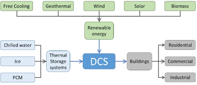
These advances and the flexibility of these systems offer the opportunity to integrate different technologies for the production and storage of cold utilities to serve the most diverse kind of clients. The production of chilled water can be achieved by different methods, which includes the use of Absorption refrigeration machines, compression equipment and combinations of mechanic and thermal driven absorption systems [25], or via “free cooling” which refers to cold water from deep lakes, rivers, aquifers or the ocean [26]. Moreover, these systems can be powered with renewable energy options like wind, solar energy, biomass, and geothermal [27]. For thermal storage, it is possible to use, chilled water tanks, ice and phase change materials (PCM). Figure 1-4 details the relationship between the production of the cold utility, and the storage technologies with different kinds of users connected to a DCS as presented by Gang et al. [27]. Cooling networks can also be integrated with Combined Heat and Power (CHP) systems to develop three-generation systems, known as Combined Cold Heat and Power systems (CCHP), which supplies electricity, hot and cold services to the users [28].

19

Figure 1-4. Flexibility and integration of technologies in DCS

District cooling interest and expansion is currently increasing around the world. In the Middle East, this growing is notorious in the Gulf region, where its evolution is exponential since the 1990s, with plans to triplicate their capacity by 2030. In the United States, some local legislation has changed to favour the implementation of these technologies, including subsidies aiming to a demand increment of district cooling. In China, DCS is still a growing industry. India is aiming to implement district cooling in five of its major cities with the support of the United Nations Environmental Program (UNEP) [29]. Additionally, district cooling can bring important benefits to society including the reduction of CO2 and

environmental hazardous refrigerants (HCFC), improvement of building environments (space and reduction of noise), reduction of peak electrical consumption in summer (guarantying local reliability of electricity supply). More benefits of the implementation of district cooling are detailed in the European report [30]. However, district cooling presents also some drawbacks including the fact that some isolated areas could not be efficiently connected to these networks and the high capital cost that might be required for their implementation [7].

1.2.1.1 District Cooling in Europe

District cooling has been developing around the most populated cities in Europe, to supply mainly the service sector, and in some cases the residential and industrial sectors [31]. By 2006, the continent reported 115 cooling systems, as detailed in Figure 1-5. In some of the European countries, the development of district cooling might depend on the previous experiences they have with district cooling like in Paris, Helsinki and Stockholm. In other cases, the development is more recent and rooted to innovate local urban projects like in Barcelona and Lisbon [30].

20

Figure 1-5. Mapping of district cooling in Europe in 2006 (biggest per country have a star) as presented in ref.[30]

As reported in 2015 by the European Commission, the total installed capacity of district cooling is 2.4 GW, which represents less than 1% of the installed district heating capacity of 301.5 GW in the region, due to the difference of demand between these two services. The largest district cooling capacities are in France (669 MW), Sweden (650 MW), Spain (317 MW), Finland (247 MW), Italy (172 MW) and Germany (168 MW). Austria (55 MW), Poland (35 MW), Denmark (34 MW) and Hungary (7 MW) also have district cooling systems. Moreover by 2011 two thirds of the energy delivered by these systems took place in France and Sweden.

Considering these facts and the cooling demands for 2015 reported by Persson and Werner for residential and service sectors (Figure 1-6) [32], we can evidence that there is a big need for the development of district cooling in all the region. France and Sweden as leaders in the implementation of district cooling, are in contrast 14th _{and 23}rd _{in the rank of cooling demand, while countries with}

21

Figure 1-6. Specific cooling demands by country, based on data in ref[32]

Due to increment and trends of useful floor areas that are cooled, and/or air-conditioned in the continent over the last few years, a sharp increment in the cooling demand is expected by 2020. The Global CCS Institute reports an increase of 82% in the cooling demand of the residential sector and 60% in the service sector for the period 2007-2020. For 2020, the saturation rates of these sectors will be of 40% and 60% respectively. Additional expansion might be caused by an increment in overall occupied floor space, climate changes and additional technical installations. Variations in building standards and social behaviour might also affect this increment. Taking this into account, a substantial increment in cooling demand is expected from 2020 to 2030 (6%).

The eventual implementation of district cooling to cover 25% of the European Cooling market, would lead to a reduction between 50 to 60TWh in the annual electricity consumption [13], resulting also in a reduction of investments in electricity capacity by 30 million €. In addition, the reduction of annual CO2 savings would be up 60 million tons, which represent 15% of the European Union’s Kyoto

commitment [30].

1.2.1.2 Penetration of district cooling in France

According to the 2018 survey of FEDENE (Fédération des Services Energie Environnement) [33], France has a total installed capacity of district cooling systems (DCS) of 1 TWh, becoming one of the most extensive systems in Europe. Nevertheless, the implementation of these systems along the country is not as widespread as for district heating systems (DHS) as detailed in Figure 1-7 and Table 1-1

22

Figure 1-7. Indicative mapping of DHS (left) and DCS (right) in France[33]

Table 1-1 details the distribution of heating and cooling networks in the country according to the survey.

Table 1-1. Distribution of heating and cooling networks in France

Heating networks Cooling networks

Number of networks 761 23

Total length of networks 5397 km 198 km

Delivered power 25 TWh 1 TWh

Buildings connected 38212 1234

This shows that although the development of district cooling networks in the systems in the country is one of the highest of the continent, there is still opportunity to increase its implementation mainly in the regions away from the big cities.

As seen in the map of Figure 1-7, Paris concentrates much of the cooling potential of the country, but it should be added that Paris also represents one of the leaders on district cooling in the world [34]. The development of district cooling in this city dates from 1968 when a centralized heating and cooling system was built as part of the renovation of the area where the shopping centre of Forum Les Halles is located today. To achieve economic feasibility, the system had to supply other buildings, and they decided to connect the Louvre museum. In this early stage of development, the system produced the cold from centrifugal chillers with cooling towers installed on the top of the building, coupled with ice energy storage. As the system expanded, with more clients, connections and production sites, its economic feasibility raised up [35]. In 1991 Climespace [36], became a shareholder with the intention of expanding the District cooling system of Paris.

23

Today, this city has developed the largest cooling network of Europe, part of which uses the Seine river for cooling [7]. The 10 production sites and the 3 storage centres meet the cooling requirements of hotels, department stores, offices, state-building and museums. The 75 km long network serves more than 650 customers with an equivalent area of 6 million m2 _[37].

24

1.2.2 Challenges on research in District Cooling

Due to its growing importance, demand and market, in the last 20 years the studies on district cooling have considerably increased [14]. The topics of growing interests include the integration of these systems with sustainable energy technologies and the optimization of its planning design and operation [27].

Literature states the use of thermal storage systems in DCS, but few studies addressed the design and control optimization of the integrated system. Problems including the optimal size of the storage system and the amount of energy to be stored need to be further investigated. The performance in different climate areas needs more studies as well as the comparison with traditional cooling systems. Rational design and planning of energy systems have an essential role to achieve energy saving/efficiency and maximum economic benefits of its implementation. Nevertheless, to accomplish these goals it is necessary to deal with [38]:

1. Spatial and temporal aspects, related to the location and consumption (power demand, temperature level), production and price profiles respectively.

2. High variety and number of network layouts and size of energy systems as possible candidates. One of the reported drawbacks for the implementation of district cooling relies on the limited knowledge of Know-how and technical skills [11], and some authors have highlighted the need to focus research on technologies and policies necessary to economic transition from single user systems to district [10].

Moreover, in the field of modelling and simulation of this systems, there are still improvements to be made regarding the coupling building-level models with system models of components (pumps, pipes), as well as a shift to fully dynamic models [39]. Finally, studies on control optimization of the entire chilled water system including DCS and users, considering dynamic character and interactions [27] and minimization of costs could improve the development of this technology.

25

1.3 Dynamic modelling and simulation in DHC

Most of the available literature on dynamic modelling and optimization of district energy systems centre their interest in the analysis of district heating systems. Nevertheless, these models can be applied to district cooling, but the following differences should be considered [40]:

➢ The smaller temperature difference in the case of DC between supply and return pipes compared with DH.

➢ Even slight changes in network temperatures (e.g. 0.1K) can have an influence on the efficiency of cooling generation.

➢ The direction of heat fluxes through the walls of buried pipes can change during the year (heat gains or losses) as the network temperature is in the range of the soil temperature

Studies on equation-based methods for the analysis of energy networks [41]–[45], use a one-dimensional heat transfer equation to describe the temperature transients in the pipes [46] that is defined as: ρ𝑐𝑓∙ 𝐶𝑝𝑐𝑓∙ 𝐴𝑝 ∙ 𝜕𝑇 𝜕𝑡 ⏞ 1 + 𝑚̇𝑐𝑓 ∙ 𝐶𝑝𝑐𝑓∙ 𝜕𝑇 𝜕𝑥 ⏞ 2 = 𝑘𝑐𝑓∙ 𝐴𝑝 ∙ 𝜕2_𝑇 𝜕𝑥2 ⏞ 3 +𝑇𝑠− 𝑇 𝑅′ ⏞ 4 (1-1)

Where ρ𝑐𝑓, 𝐶𝑝𝑐𝑓, 𝐴𝑝, and 𝑚̇𝑐𝑓 are the density, specific heat capacity, cross-section area, and mass

flow rate of cooling fluid in the pipe, respectively. 𝑘𝑐𝑓 and 𝑅′ are the thermal conductivity of the

cooling fluid and the total thermal resistance per unit length of pipe; 𝑇 stands for temperature in the pipe, 𝑇𝑠 for the temperature of the soil surface, and 𝑡 and 𝑥 for time and distance variables. The groups

1 to 4 in equation (1-1) represent the gains, the enthalpy flux, conductive and convective heat transfer of the fluid.

This heat equation is subject to the following assumptions: ✓ Plug flow

✓ The heat transfer is considered only in the radial direction

✓ Conduction heat transfer is considered through the pipe, the insulation, the casing and the soil ✓ Material properties are constant and independent of temperature.

✓ It does not include thermal interactions between supply and return pipes ✓ Thermal inertia of the pipes, the casing and the insulation is neglected

The term of conductive heat transfer in the fluid (3) is negligible compared to the other components of the equation and can be neglected [44]

26

The computation of the total thermal resistance 𝑅′ is a function of the thermal conductivities of the pipe, the insulation, the casing and the soil respectively as well as the flow regimen of the pipe (through the internal convection heat transfer coefficient) and is given by [42]:

𝑅′₌ 1 2𝜋𝑟𝑎ℎ̅ + ln (𝑟_𝑟𝑏 𝑎) 2𝜋𝑘𝑎𝑏 + ln (_𝑟𝑟𝑐 𝑏) 2𝜋𝑘𝑏𝑐 + ln (𝑟_𝑟𝑑 𝑐) 2𝜋𝑘𝑐𝑑 + 1 𝑆𝑘𝑠 (1-2)

Figure 1-9. Representation of a buried pipe

Where ℎ̅ is the average convection heat transfer coefficient in the pipe; 𝑘𝑎𝑏, 𝑘𝑏𝑐, 𝑘𝑐𝑑, and 𝑘𝑠 are the

thermal conductivities of the pipe, insulation, casing, and soil, respectively and S is the conduction shape factor, that can be approximated as [46]:

𝑆 = 2𝜋𝐿

ln (_2𝑟4𝑑

𝑑)

(1-3) For 𝑑 > 3𝑟𝑑

The average convective heat transfer coefficient is computed as: ℎ̅ =𝑁𝑢̅̅̅̅𝑘𝑐𝑓

2𝑟𝑎

(1-4) Where 𝑁𝑢̅̅̅̅ is the local Nusselt number assuming turbulent flow in a smooth circular tube and can be computed from the Dittus-Boelter equation as[47]:

𝑁𝑢 = 0.023𝑅𝑒4/5_𝑃𝑟0.4 _(1-5)

Finally, Reynolds and Prandtl's numbers are represented by: 𝑅𝑒 =𝜌𝑐𝑓𝑣 ∙ 2𝑟𝑎 𝜇𝑐𝑓 (1-6) 𝑃𝑟 =(𝐶𝑝𝑐𝑓𝜇𝑐𝑓) 𝑘𝑐𝑓 (1-7)

27

Where 𝑣 is the flow velocity, 𝜇𝑐𝑓 is the dynamic viscosity of the cooling fluid. The presented partial

differential equation has been used for the dynamic of district heating systems, but as stated at the beginning of the section it can be applied to study district cooling systems.

The solution of the Partial Differential Equation (PDE) (1-1) can be addressed using discretization strategies (e.g. Finite elements, finite volumes, finite differences) or 1D analytical solutions coupled with physical approximations.

Using partial discretization, the PDE becomes a system of ordinary differential equations (ODE) that can be solved using a numerical integrator implementing a method such as Runge-Kutta. While using total discretization, the PDE becomes a set of algebraic equations. Among the approximations using discretization strategies, Ben Hassine et al. [41] implemented explicit finite differences of 1st _order

(𝜕𝑇(𝑥,𝑡) 𝜕𝑥 = 𝑇(𝑥,𝑡)−𝑇(𝑥−∆𝑥,𝑡) ∆𝑥 , 𝜕𝑇(𝑥,𝑡) 𝜕𝑡 = 𝑇(𝑥,𝑡)−𝑇(𝑥,𝑡−∆𝑡)

∆𝑡 ) to fully discretize the PDE resulting into a system

of nonlinear equations that can be solved explicitly. They present a quasi-dynamic approach, implemented in Matlab®, where the flow and pressure in the network are calculated using a static flow model, and the temperature is calculated dynamically

On the other hand, there are estimations based on a succession of steady states, as proposed by Duquette et al. [42], or the Lagrangian approach of other authors [43]. The first ones solve the equation (1-1) analytically in steady-state, finding an expression that computes the outlet temperature. In this case, the integration of the temperature is performed along the length of the pipe. Then, a transport delay is computed to simulate the fluid flow in the pipe using a numerical time series model, implemented in Simulink®. At each time step, a new estimate of the transport delay is computed (since the mass flow is time-dependent) and stored. Hence, the fluid temperature at the pipe outlet considering the transport delay is calculated, enabling to model the propagation of the temperature in the pipe. This implementation is attractive in terms of computational time, nevertheless, due to the storage of data and the growing of the model during the simulations it is not suitable for optimization applications. Besides, the implementation focused only on the distribution network and no indication was given on how to extend the methodology to model the users or the heat/cold producer. Other authors use an equivalent approach, which analytically solves the Lagrangian (material) derivative over time (also known as the method of characteristics). In this case, the integration of the temperature is made from the initial time to the value of the final time that includes the transport delay. The latter is computed using the velocity in the pipe which is linked to the mass flow that can be constant or variable as stated by Velut and Tummescheit. Van der Heijde et al. [44] and Schweiger et al. [45] perform this implementation in Modelica®, where the calculation of the fluid and temperature propagation are separated from the heat loss calculation, combining a plug flow approach with an ideal mixed volume model.

28

1.4 Optimization approaches

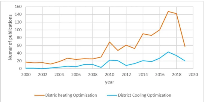
The optimization of district energy systems is strongly motivated by minimizing the cost of infrastructure and the emissions maximizing the production of the hot or cold utility, or its efficiency. Such optimization is particularly challenging because of technical characteristics and the size of real-world applications [38]. In general, mathematical optimization of these systems is strongly unbalanced in favour of the analysis of district heating systems, as stayed by Werner [14] and evidenced in the number of publications registered in the Elsevier’s abstract and citation database Scopus between January 2000 and March 2019 for each kind of system. Figure 1-10 compares the number of publications in the mentioned period registered in the Scopus database when searching for “district heating optimization” (1062 documents) and “district cooling optimization” (271 documents).

Figure 1-10. Comparison of research in Optimization of district heating and district cooling systems

It is important to point out that each kind of systems presents its own issues, related not only with the kind of utility produced (hot or cold) but also with its operation for improving the system efficiency, as it will be detailed in the objectives of this work.

These facts highlight the importance of studies focused on district cooling networks. But despite the lack of analysis of district cooling systems, it is important to highlight that most of the methodologies implemented for the different analysis in DHS can be used to study DCS as well.

Before introducing the applications of optimization in district energy systems, it is important to present a general classification of the type of problems we find in mathematical optimization. An optimization problem consists of one (or sometimes more) objective function to be minimized (e.g.

29

Operational cost, CO2 emissions) or maximized (efficiency, production), subject to the fulfilment of

physical or operational constraints of the system, represented as equality or inequality constraints, by manipulating a set of decision variables. Depending on the nature of the decision variables (continuous or discrete), it is possible to establish a general categorization of optimization problems, that is independent of the methods implemented to solve the problem as stated by Biegler and Grossmann [48]. If the problem is described only by continuous variables, considering the nature of the constraints and the objective function that describes the system (linear or non-linear) we have linear programming (LP) and non-linear programming (NLP) problems. When discrete variables are involved, they are classified as mixed-integer linear programming (MILP) and mixed-integer non-linear programming (MINLP) problems. Finally, when dealing with dynamic models, two approaches are possible. Either we represent the dynamic problem as a succession of steady-state problems known as multi-period optimization, or we actually deal with the dynamic of the system. In this latter, we can do this either via the Pontryagin’s principle (optimal control) or via discretization, formulating the dynamic problem as an algebraic problem (NLP, MILP or MINLP) known as dynamic optimization.

Following the presented classification, we can organise the studies on the optimization of district heating and cooling as presented in Table 1-2. The table details selected contributions in terms of the kind of problem that is solved and their main applications. More extensive reviews on the applications of optimization in District energy systems are presented by Talebi et al. [49] Sameti et al. [38], Gang

et al. [27]. Eveloy and Ayou[19] also present optimization applications specifically for DC, highlighting

that most of the studies have focused on the optimization of the distribution network infrastructure (MILP and MINLP formulations) considering steady-state models.

Table 1-2. Classification of works on Optimization of DHC

Continuous Variables Integer variables

NLP MILP MINLP Data based Chow et al.[50] - Diversity factor Data based Deng et al.[51] -Scheduling Steady-state Söderman[52] - Topology

- Operation (flow rates)

Steady State Mertz et al.[53] Marty et al.[54] - Topology - Sizing - Operation Multiperiod Khir et al. [55] - Sizing - Topology

30

Continuous Variables Integer variables

NLP MILP MINLP

- Operation Dynamic

Schweiger et al.[45] - Operation Powel and Edgar[56]

- Temperature control Powel et al[57] - Operation This contribution - Operation - Pipe diameters

Dynamic data based MIQCP Schweiger et al.[45]

- Scheduling

Due to the complexity involved in the models to describe these systems, the applications of LP in district heating and cooling are scarce.

Most of the applications are focused on the optimization of the distribution network infrastructure that includes the selection of technologies, the number and kinds of users connected to the network, existence of network elements (pumps, chillers, storage tanks, pipes), that results in implementations with integer variables (MILP and MINLP).

Among the application in district cooling, Chow et al. [50] presented a MILP formulation that optimized the diversity factor, which is the proportion of diverse types of buildings (Office, Residential, shops, hotels and mass transit railway stations) leading to a uniform cooling load to ensure a high stability to the cold production system to be installed. They first calculate 24 hourly typical profiles of demands for five types of buildings using a freeware building energy analysis program that can predict the energy use and cost for all types of buildings, for 36 typical days (three typical days per month). Then, with these data, they implemented a genetic algorithm to solve a MILP problem that aims to minimize a fluctuation index with respect to the maximum cooling demand. Here the optimization variables are the number of buildings for each of the five categories. In order to try to avoid local optima, they used a genetic algorithm. However, their study does not consider the topology of the network, which might have an important impact on the delay and in the formulation of the fluctuation index.