Dynamic retail assortment models with demand learning for seasonal consumer goods

Dynamic Retail Assortment Models with Demand

Learning for Seasonal Consumer Goods

by

Felipe Caro

Civil Industrial Engineer, University of Chile (1999)

Submitted to the Sloan School of Management

in partial fulfillment of the requirements for the degree of

MASSACHUSETTS INwS!-TWE

Doctor of Philosophy in Management

at the AUG 0 9 2005

MASSACHUSETTS INSTITUTE OF TECHNOLOG

LIBRARIES

June 2005

®

Felipe Caro, MMV. All rights reserved.

The author hereby grants to MIT permission to reproduce and

distribute publicly paper and electronic copies of this thesis document

in whole or in part.

Author

... a...

-

.

i....

.... ..

Sloan School of Management

<~ra

April 29, 2005

Certified

by ...

...

__ ----"---- Jrmie Gallien

J. Spencer Standish Career Development Professor

Thesis Supervisor

Accepted

by ...

...

Birger Wernerfelt

Professor of Management Science

for Seasonal Consumer Goods

by

Felipe Caro

Submitted to the Sloan School of Management on April 29, 2005, in partial fulfillment of the

requirements for the degree of

Doctor of Philosophy in Operations Management

Abstract

The main research question we explore in this dissertation is: How should a retailer modify its product assortment over time in order to maximize overall profits for a given selling season?

Historically, long development, procurement, and production lead times have con-strained fashion retailers to make supply and assortment decisions well in advance of the selling season, when only limited and uncertain demand information is available. As a result, many retailers are seemingly cursed with simultaneously missing sales for want of popular products, while having to use markdowns in order to sell the many unpopular products still accumulating in their stores.

Recently however, a few innovative firms, such as Spain-based Zara, Mango and Japan-based World Co. (referred to as "Fast Fashion" retailers), have gone substan-tially further, implementing product development processes and supply chain archi-tectures allowing them to make most product design and assortment decisions during the selling season. Remarkably, their higher flexibility and responsiveness is partly achieved through an increased reliance on more costly local production relative to the supply networks of more traditional retailers.

At the operational level, leveraging the ability to introduce and test new products once the season has started motivates a new and important decision problem, which seems crucial to the success of these fast-fashion companies: given the constantly evolving demand information available, which products should be included in the as-sortment at each point in time? The problem just described seems challenging, in part because it relates to the classical trade-off known as exploration versus exploitation, usually represented via the multiarmed bandit problem.

In this thesis we analyze the dynamic assortment problem under different sets of assumptions, including: (i) without lost sales; (ii) with lost sales but observable demand; (iii) with lost sales and censored information; and (iv) with time vary-ing demand rates. In each case we formulate an appropriate model and suggest a (near-optimal) policy that can be implemented in practice, together with associated suboptimality bounds. We also study the incorporation of substitution effects and

the extension of the models to a generic family of demand distributions. The com-mon solution approach involves the Lagrangian relaxation and the decomposition of weakly coupled dynamic programs.

The dissertation makes three contributions: (1) it is the first attempt in providing mathematical optimization models with near-optimal solutions for the dynamic as-sortment problem faced by a fast-fashion retailer; (2) our analysis contributes to the literature on the multiarmed bandit problem, in particular for its finite-horizon ver-sion, we derive a general closed-form dynamic index policy that performs remarkably well; and (3) the solution approach contributes to the emerging literature on duality in dynamic programming.

Thesis Supervisor: Jremie Gallien

I have reached the end of my studies at MIT and I cannot submit this thesis without expressing my gratefulness to all the people that have been next to me during these splendid years in Cambridge.

First, I would like to thank my advisor Jremie Gallien for getting me involved in the fascinating research project that became my thesis. This work owes a lot to his support and guidance, and for me it has been career defining. I am still amazed on how fast everything worked out. I guess he had it all clear and well planned in his mind. Lucky me. Merci beaucoup!

I also want to thank the other members of my Thesis Committee, Professors Stephen Graves and Gabriel Bitran. It was an honor to have you in my committee and it was a privilege to have my office (or closet?) right next to yours. I admire your academic work and I really appreciate all the feedback and experience you shared with me.

At MIT I had the opportunity to learn from and interact with many faculty and staff members that made these years a formidable and enriching experience. In particular, I thank Professor David Simchi-Levi for his support during my first years. I hope that we continue to collaborate in the future.

MIT is a remarkable place and I would say that its best treasure is the quality of the students it attracts. I have learned almost as much from my classmates than from my professor. But besides the research, MIT is also a great place to make friends, and I made lots of them. To begin with, I have to thank Herman Bennett for being an excellent comrade from day one. My friend Victor Martinez-de-Albeniz deserves a similar distinction. Then I want to thank my OM classmates and the smart guys from the OR Center. The list is long (should I put an online appendix?).

Beyond the MIT campus I also met many people that cheered up the evenings and weekends. In particular I thank the partygoers that attended the Pub Tours on Thursdays: Cornelius, Matteo, Manu, Eva, Jitkee, Hui, Caroline, Marta, Raf, Seb, and many others with whom I shared a beer. Yeah, despite the stress, we had a lot of fun. Outside the party scene, I thank Alejandro Conejero, Daniel Hojman and Paulina Achurra for the good company, and Joe Doherty for being like family here.

Well, I have said enough about MIT and how much I loved living in Boston, but now I go down to Earth. For any achievement in my life, I must thank my parents, Rodrigo y Ximena, my sister Loreto and my brother Javier. Your love has allowed me to get where I am, without forgetting what are the really important things in life. Los quiero mucho.

Coming from Chile, I also want to thank the Department of Industrial Engineering of the University of Chile, in particular, my colleagues and academic mentors Andres Weintraub and Rafael Epstein.

Finally, last but not least, the most important acknowledgement is for my dearly loved Marcela. I am extremely happy that you became part of this story, and with you I want to celebrate the most. Needless to say, my Ph.D. dissertation is dedicated to you.

1 Introduction 1.1 Motivation . 1.2 Literature Review 10

... . 10

... . 13

2 Duality Results for Dynamic Programs

2.1 The Dual DP ...

2.2 Open-Loop Dual Policies ...

16

17 18

3 Model without Lost Sales

3.1 Model Definition. 3.1.1 Supply.

3.1.2 Demand ...

3.1.3 Dynamic Programming Formulation ... 3.2 Model Discussion.

3.3 Analysis ...

3.3.1 Properties of the Profit-to-go Function .... 3.3.2 Remarks on the Dual Dynamic Program . . . 3.3.3 Single Product Subproblem ...

3.3.4 The Index Policy ...

3.3.5 Assortment Implementation Lead Time .... 3.4 Demand Distribution from the Exponential Family 3.5 Numerical Experiments.

3.5.1 Methodology.

3.5.2 Bayesian Experiments. 3.5.3 Frequentist Experiments. 3.5.4 Assortment Rotation.

3.5.5 Sensibility Analysis with Respect to S and N 3.5.6 Response Surface Bandits ...

23 23 23 24 25 26 29 30 32 34 40 45 47 47 50 54 57 59 60 . . . ..I : :

4 Incorporating Substitution Effects 4.1 Heuristic Procedure . 4.2 Numerical Experiments . 63 63 65

5 Models with Lost Sales 71

5.1 Total Demand is Observable ... 72

5.1.1 Model Definition ... 73

5.1.2 Numerical Experiments ... 76

5.2 Censored Information ... 77

6 Conclusions and Extensions 81 6.1 Concluding Remarks ... 81

6.2 Model Extensions and Future Work ... 83

6.2.1 The Multiarmed Bandit Beyond Retailing ... . 83

6.2.2 6.2.3 Lost Sales Model when Stock-out Epochs are Model with Variable Demand Rates ... Observable 6.2.4 Multiple Stores, Endogenous Demand, and Other Extensions . A On the concavity of ft(C) B Proofs B.1 Proof of Proposition 1 B.2 Proof of Proposition 2 B.3 Proof of Lemma 1 . . . B.4 Proof of Lemma 2 . . . B.5 Proof of Lemma 3 . . . B.6 Proof of Lemma 4 . . B.7 Proof of Proposition 3 B.8 Proof of Proposition 4 B.9 Proof of Lemma 5 . . . 84 85 86 89 92 . . . 92 . . . 92 . . . 94 . . . 95 . . . 95 . . . 98 . . . 98 . . . .101 . . . .102

1-1 The dynamic assortment problem ... 12

3-1 The threshold functions when A3 > 2> A1. . ... . . 34

3-2 Plot of Zt as a function of t. ... 36

3-3 Graphical representation of the proposed index policy ... 39

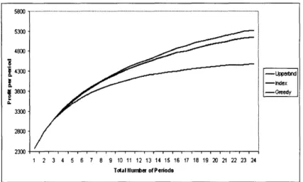
3-4 Relative policy performance for various horizon lengths . . ... 52

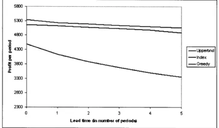
3-5 Relative policy performance for various lead times. ... 53

3-6 Assortment rotation with active and passive learning (N = 30). .... 58

3-7 Sensibility analysis with respect to S and N .. ... 60

4-1 Simple substitution structures. . . . .. . 66

4-2 One-item substitution. ... 68

4-3 Adjacent substitution. ... 69

4-4 Random substitution ... 70

List of Tables

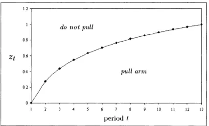
3.1 First values of zt ... 36

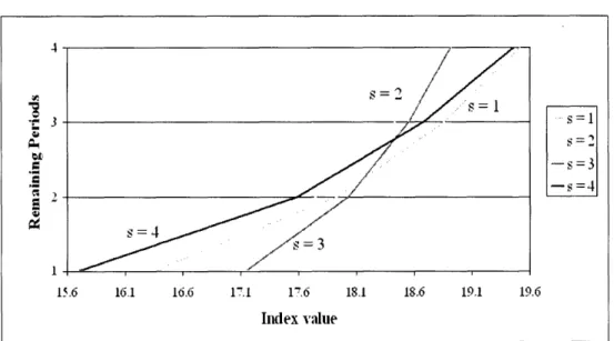
3.2 Data of the example in Figure 3-3. ... 39

3.3 Bounds of Lemma 2 ... .. 49

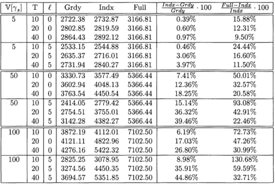
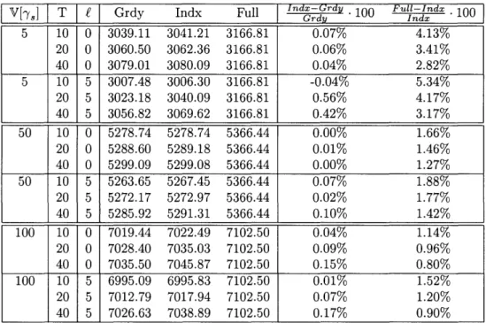
3.4 Index policy vs. greedy rule (Bayesian approach) ... 51

3.5 Index policy vs. greedy rule (frequentist approach). ... 55

3.6 Relative policy performance with improved accuracy of initial

informa-tion

.

.. ...

.

...

56

3.7 Relative policy performance with biased initial information ... 56

3.8 Assortment rotation . .... ... .58

3.9 Approximate Gittins index vs response surface index ... 61

4.1 Simulation running times for adjacent substitution (rounded to seconds). 70 5.1 Active vs. passive learning with lost sales ... 76

Introduction

1.1 Motivation

Long development, procurement, and production lead times resulting in part from a widespread reliance on overseas suppliers have traditionally constrained fashion re-tailers to make supply and assortment decisions well in advance of the selling season, when only limited and uncertain demand information is available. With only little ability to modify product assortments and order quantities after the season starts and demand forecasts can be refined, many retailers are seemingly cursed with simulta-neously missing sales for want of popular products, while having to use markdowns in order to sell the many unpopular products still accumulating in their stores (see Fisher et al. 2000).

Since the late 1980's an industry-wide initiative known as "Quick Response" (see Hammond 1990 for a more detailed description) has focused on attenuating that curse, meeting some success. Leveraging information technologies, improved product designs and manufacturing schemes as well as faster transportation modes, some of its followers have significantly improved the flexibility of their overseas supply networks, thus managing to postpone part of their production until more demand information can be gathered.

Recently however, a few innovative firms including Spain-based Zara, Mango and Japan-based World Co. (sometimes referred to as "Fast Fashion" companies) have gone substantially further, implementing product development processes and supply chain architectures allowing them to make most product design and assortment de-cisions during the selling season. Remarkably, their higher flexibility and

responsive-Chapter 1. Introduction

ness is partly achieved through an increased reliance on more costly local production relative to the supply networks of more traditional retailers. The contrast between these two supply-chain design alternatives seems particularly drastic: Zara's design-to-shelf lead time range for new or modified product is 2 - 5 weeks, versus 6 - 9 months for a more traditional retailer; in-house production during the season is re-ported to be approximately 85% for Zara, versus less than 20% for other retailers; Zara manufactures about 11, 000 different products per year (excluding variations in color, size and fabric), compared to only 2, 000-4, 000 items for key competitors; only 15 - 20% of Zara's sales are typically generated at marked-down prices, compared with 30 - 40% for most of its European peers, furthermore the percentage discount for their marked-down items was estimated as roughly half of the 30% average for other European apparel retailers (see Ghemawat and Nueno 2003).

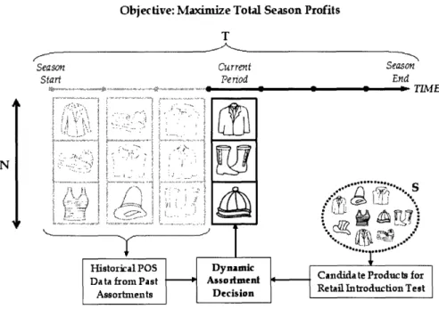
At the operational level, leveraging the ability to introduce and test new products once the season has started motivates a new and important decision problem, which seems key to the success of these fast-fashion companies: given the constantly evolving demand information available, which products should be included in the assortment at each point in time? Figure 1-1 provides a conceptual representation of this operational challenge: in each period over a finite horizon (representing the whole season T), the retailer must decide the subset (N) of products that will be offered from a larger set (S) of all retail introduction candidates. As sales occur, the retailer gathers new demand information about each particular product that was included in the latest assortment, which may be combined with prior historical demand information to select the next assortment - although not shown in Figure 1-1 for simplicity, it must be noted that the assortment decision can typically only be implemented after a lag (k?) corresponding to the design-to-shelves lead time.

The problem just described seems challenging, in part because it relates to the classical trade-off known as exploration versus exploitation: in each period the retailer must choose between including in the assortment products for which he has a "good sense" that they are profitable (exploitation), or products for which he would like to gather more demand information (exploration); that is, he must decide between being "greedy" based on his current information, or try to learn more about product demand (which might be more profitable in the future). In addition, this problem poses itself frequently, for a high number of products, and involves a large amount of data. Incidentally, we only have limited understanding at present of how these companies

Objective: Maximize Total Season Profits

N

T

Season Current Season Start Pe riod End

Historical POS Dynamic Candidate s or

I :

' ;'.

.

,

Assortments _{Assortmnts ~ A rDecison} Retail Introduction Test

E

Figure 1-1: The dynamic assortment problem.

actually solve this dynamic assortment problem in practice, and all studies focusing on fast-fashion companies we are aware of (e.g. Fisher et al. 2000, Ghemawat and Nueno 2003, and Ferdows et al. 2003) only describe this challenge in qualitative terms. Our main objective in the present paper is thus to develop and analyze a quantitative optimization model capturing the main features of this dynamic assortment problem, with a view towards eventually creating an operational decision support system.

The remainder is organized as follows: in Chapter 2 we provide all the duality results for dynamic programming that are used throughout the thesis. In Chapter 3 we present the basic dynamic assortment model under the following salient assump-tions: (i) the demand process for each individual product is independent of the other products; (ii) there are no lost sales; and (iii) the demand rates remain constant dur-ing the selldur-ing season. Chapter 4 shows how substitution effects can be taken into account, and Chapter 5 covers the models that consider inventory decisions. Finally, in Chapter 6 we provide concluding remarks and discuss other model extensions.

Chapter 1. Introduction

1.2 Literature Review

We first discuss papers focusing on assortment problems. A first subset is found in the Marketing literature, where several studies, typically motivated by supermarkets, consider static assortment problems formulated as deterministic nonlinear optimiza-tion models in which the demand of a product depends on the allocated shelf space, and the overall space available is a limited resource. A classical example in this vein is Bultez and Naert (1988); for more recent work see Kok and Fisher (2004) and ref-erences therein. In the Operations Management literature, van Ryzin and Mahajan (1999) and Smith and Agrawal (2000) are two papers also considering static assort-ment problems, but with a stochastic demand model and static product substitution. That is, customer demand reflects aggregated substitution effects depending on the initial assortment decision, but not on the actual inventory levels observed by individ-ual customers once arrived to the store. In contrast, Mahajan and van Ryzin (2001) describe a more detailed assortment model capturing dynamic substitutions, that is substitutions due to stockouts experienced by individual customers, and analyze it using sample path methods.

None of the papers just cited considers demand learning, and accordingly the assortment problems they investigate are static, not dynamic. Presumably because of the relative novelty of fast fashion companies, we have in fact not found in the literature any dynamic assortment model explicitly described as such. While papers underlying the quick response initiative described in the previous section do place much emphasis on learning and exploiting early sales information, the demand infor-mation acquired over time is primarily exploited by the manufacturer to make better ordering and production quantities decisions, as opposed to product design or assort-ment decisions; the seminal paper by Fisher and Raman (1996), motivated by skiwear manufacturer Sport Obermeyer, presents a two-stage stochastic programming model in which initial production commitments are made before any sales occur, but fur-ther production decisions are made in a second stage after receiving some customer orders and refining total sales forecasts. Note that the trade-off between exploration and exploitation is not present in the problem just described, where in fact the

opti-mal policy consists of postponing the ordering of products for which demand is most uncertain.

As may already be clear from Figure 1-1, our work is closely related to the mul-tiarmed bandit problem, which has been extensively studied in the literature (see

Berry and Fristedt 1985, Kumar 1985, and Brezzi and Lai 2002). In the discrete-time version, a player chooses N arms to pull out of a total of S available in each one of T periods. Whenever pulled, each arm generates a stochastic reward following an arm-dependent distribution, which is initially unknown but can be inferred with experience as successive rewards are observed; the player's objective is to maximize total reward over the game horizon. In the present paper, pulling an arm is equivalent to including in the assortment the product to which it is associated.

A remarkable result for the multiarmed bandit problem is due to Gittins (see Gittins and Jones 1974, and Gittins 1979). It involves the definition of the so-called Gittins' index for each arm s, equal to the lump sum that would make the player indifferent between retiring or playing arm s individually, ignoring the other arms (cf. Bertsekas 2001, Vol. II, pp. 60-70). Assuming independent arms, infinite horizon

(T = oc), exactly one arm pulled in each stage (N = 1) and a discount factor strictly smaller than one, the optimal policy is to play in each stage the arm with the highest Gittins' index. Among several subsequent extensions to Gittins' result we highlight the work on restless bandits by Whittle (1988), whose analysis is related to ours in that it also involves Lagrangian multipliers.

In the finite horizon case (T < oc), it is known that Gittins' index policy is in general not optimal. Relevant references include the book by Berry and Fristedt (1985), which presents analytical techniques similar to the ones we use in the next sections. Lai (1987) develops a policy (or allocation rule) based on the calculation of an upper confidence bound for each arm (which can also be seen as an index). For the case with multiple plays per stage, Anantharam et al. (1987) consider the frequentist version of the problem, where the objective is to minimizing regret. While the allocation rule they propose is asymptotically efficient, it does not seem directly applicable to our problem because it requires a setup phase of at least S x N periods in order to have N initial observations per arm, and does not allow for a response lag (stemming in our context from the design-to-shelf lead times).

In §3.3.5 we introduce an assortment implementation lag to our model so it be-comes equivalent to a finite horizon multiarmed bandit with a response delay. The amount of literature available for this variant of the classic problem is rather limited. Most of the papers come from the statistics community that is interested in the ap-plication to clinical trials. However, the typical model involves only two arms with Bernoulli rewards. A good example is the recent work by Hardwick et al. (2005),

Chapter 1. Introduction 15

where the response delay has an exponential distribution (in our case the lag is con-stant and measured in number of periods).

Finally, the paper by Bertsimas and Mersereau (2004), which focuses on an adap-tive sampling problem, is the reference that is methodologically closest to our work - their model is a finite horizon version of the multiarmed bandit problem, and their analysis also involves Lagrangian decomposition. However, they do not consider response lags and assume a Beta-Bernoulli learning model, while we use the Gamma-Poisson model. Besides, in contrast to that paper we provide a suboptimality bound for the policy we derive.

Duality Results for Dynamic

Programs

Dynamic programming (DP) is the natural methodology used to model and solve sequential decision problems. However, despite its versatility, in the vast majority of cases when a closed form optimal policy is not available, the numerical solution of the model involves computational requirements that quickly become overwhelming. This fact is known to be the curse of dimensionality of DP (see Bertsekas 2001), and as a consequence, approximate solution methods are in order.

The DP models developed in this thesis are subject to the curse of dimensionality and the approximate solution approach we follow is based on Lagrangian relaxation and the decomposition of weakly coupled dynamic programs. The underlying concepts involved are similar to those of the well-established theory of duality for general nonlinear optimization problems (see for instance Bertsekas 1999). The approach dates at least from the late 80's with the independent work done by Karmarkar (1987) on a finite-horizon multilocation inventory problem, and the seminal paper of Whittle (1988) on restless bandits. The rest of the literature reporting successful applications of this methodology is rather recent, see for instance Castafion (1997), Talluri and van Ryzin (1998), Yost and Washburn (2000), Rajaram and Karmarkar (2002), Hawkins (2003), Bertsimas and Mersereau (2004), and references therein.

The results shown in the present chapter can be seen as a generalization and extension of the individual applications found in the literature.

Chapter 2. Duality Results for Dynamic Programs

2.1 The Dual DP

Under the same framework as in Puterman (1990) and Bertsekas (2001), consider the following generic finite horizon Bellman equation, in which periods are counted

backwards:

J7*(x)

= max gt(x, u)+ E,(,u) [Jtl((ot(x,u, n))] x

(2.1)

a'u<N

with J(x) = 0 V x E

Q2.

In terms of notation, bold symbols represent vectors, and in particular, x, u, and

n correspond to the state, control, and random disturbance vectors respectively (note

that index t for these quantities has been omitted for ease of notation). The state space is , and the control space is given by the intersection of U (an arbitrary set) with all the control vectors that satisfy the linear constraint a'u < N. The transition

function pt(x, u, n) captures the dynamics of the model from period t to period t- 1. The proofs we provide assume that the disturbance n takes values in a countable space (in order to avoid unnecessary technical details, see the discussion in §1.5 of Bertsekas 2001).

In our case, the linear constraint a'u < N corresponds to a shelf space constraint but in general it can be regarded as some "coupling constraint" that is conveniently relaxed, which leads to the definition of dual policies that will later prove to be useful in finding near-optimal primal policies and upper bounds for the optimal profit-to-go. Let At(x) denote any function associated with period t that maps the state space into the set of nonnegative real values; we define a dual policy to be any vector a functions

At = (t(-), At- (), * * ,

1(-))-For any dual policy At and any initial state x, the corresponding profit-to-go is

obtained by solving the dual dynamic program given by:

Ht (x) = NAt(x) + max gt(x, u)

-

At(x)a'u + IEn(,[Htl

(ot(xun))]

(2.2)

uEU '

with HA°(x) = 0 V x E 2. In words, a dual policy gives a price (Lagrange multiplier) for a unit of shelf space for each period and each possible state.

1_{We present our results in a finite-horizon framework that fits the DP model to be introduced in}

the next chapter. Analogous results can be derived for other settings, in particular, for the infinite horizon case.

A dual policy At is optimal if it minimizes the right hand side of (2.2) for any initial state. In line with standard dynamic programming theory, we recursively define

At(x) to be the smallest solution of the following dual problem:

Ht

+

n))], (2.3)

At>0 uEU

and it can be verified through straightforward induction that the policy A* is indeed optimal.

The following proposition is an intuitive result that relates the primal and dual DP's; a similar result for open-loop dual policies (to be defined shortly) can be found

in Hawkins (2003).

Proposition 1 (Weak DP Duality) For any period t, any dual policy At and any

given initial state x: Jt*(x) < H*(x) < Htt(x).

As in classical duality theory, an interesting theoretical question is to determine if the first inequality in Proposition 1 ever holds as an equality; this question is partially

solved by the following proposition:

Proposition 2 (Strong DP Duality) Consider the following parametric function:

f,(x'; C) = max gt(x', u)

+

[J*l(pt(x', u, n))]

(2.4)

a'u=C

If f,1(x'; C) is increasing and concave in C for all T t, . . . 1 and states x'

reachable from x in period T, then Jt*(x) = H (x).

In contrast with (2.1), the parametric function defined by (2.4) requires the shelf space constraint of the current period to be satisfied as an equality; the shelf space constraints for the subsequent periods remain unaltered however.

Via a counterexample, it will be shown in the next chapter that strong DP duality does not always hold. However, in the rather few cases of the dynamic assortment problem when it does not apply, the duality gap is small.

2.2 Open-Loop Dual Policies

Solving the dual DP problem given by equation (2.3) seems just as hard as solving the original primal problem (2.1), motivating further simplifications. Specifically, we now

Chapter 2. Duality Results for Dynamic Programs

restrict our attention to open-loop dual policies, in which the shadow price on shelf space is constant across all states for each period; formally an open-loop dual policy A is a constant vector (At, At-1,.. ., A1), rather than a vector of functions. We use the

name open-loop to be consistent with the usual concepts in DP theory that makes a difference between the policies that depend on the system state (closed-loop) and those that do not (see p. 4 in Bertsekas 2001). Castafion (1997) calls the closed-loop dual policies stochastic multipliers and the open-loop policies deterministic

multipli-ers. Karmarkar (1987) refers to the latter as "restricted Lagrangian".

In the following, we will use the notation H"(.), instead of HtX(.), to denote the profit-to-go corresponding to an open-loop dual policy A.

Proposition 1 implies that an upper bound for the primal problem is obtained by considering the best open-loop dual policy:

Jt (X) < min H>(x) (2.5)

A>O

A better bound follows from using the best open-loop dual policy to approximate (for each state) the profit-to-go Jt*1(t(x, u, n)) in the Bellman equation (2.1), that

is:2

Jt (x) < max t(xu) + En(x,u) [ min Ht_l (pt(x, u, n))] (2.6)

a'lu<N

However, the expectation in (2.6) is not separable and its calculation seems very computationally intensive. By interchanging the order of the minimization and max-imization operators in (2.6) we still have an upper bound and the problem becomes separable but also then equivalent to solving (2.5). The minimization with respect to A in (2.5) can be solved with any convex non-differentiable optimization method, and yields the upper performance bound that we use extensively in this thesis.

It is interesting to note that finding the best open-loop dual policy, i.e. solving (2.5), is equivalent to solve the original (primal) problem but requiring the coupling constraint to be satisfied on average in each period, instead of having it satisfied for each possible sample-path. In other words, for each period, the constraint a'u < N is replaced by E[a'u < N], where the expectation is with respect to all possible states weighted by the probability of reaching each one of them under a given (primal)

2In what follows there is a slight abuse of notation: we write A to denote a vector but the number of components depends on the context, for example when writing HtA_ 1(.) A is a vector with (t- 1) components.

policy. This fact has been observed by several authors in their particular applications (see Whittle 1988, Castafion 1997, and Talluri and van Ryzin 1998). We will show the equivalence by means of an example relevant to the dynamic assortment problem, that is the finite horizon multiarmed bandit problem with several plays per stage.

Consider S independent bandit machines. Let QS be the set of all possible states of bandit s, that for any practical purposes can be assumed to be finite. The player has T periods in which he can play (at most) N arm. If a given state i E Qs the arm

of bandit s is pulled, then the player receives a reward equal to Ri and a transition to state j E ~Q occurs with probability Pij. For simplicity (and also in agreement with the dynamic assortment problem) we assume that Ri > 0 Vi Us I= Q,. The

objective of the player is to maximize the total reward over T.

We consider the problem description in the previous paragraph to be the "original primal problem". Suppose now that the player is allowed to play (at most) N arms on average in each period. This relaxed version of the problem can be formulated as a linear program (LP). In fact, let 7r be any admissible policy (for the relaxed problem). For a given state j E QS, let j(t) be the indicator function that equals one if the

player pulls the arm of bandit s in state j at time t, and let y(7r) = E,[j(t)]. Then y (7r) is a frequency measure that represents the expected number of times the player pulls the arm of bandit j at time t under policy r. Let xT be the initial state (T = 1 if bandit s starts at state j E Qs), then the player solves the following problem:

T S

JT(xr ) = max E R3yJ(7r) (2.7)

t=l s=1 ijEs

It can be shown that problem (2.7) is equivalent to solving the following LP (see Bertsimas and Nifio-Mora 2000):

Chapter 2. Duality Results for Dynamic Programs T S J(x T ) = max Ey Rjy (2.8) t=l s=l jiEs subject to Yj -l

-j

t

=

2,...,

yJ < N

t= 1,...,T

_(2.9)

y7J

> 0

t

Vs, Vj

Q,

t =

1,.,T

The constraints (2.9) ensure that the on average the player does not pull more than N arms in every period. We now relax ("dualize") that constraint using a vector of multipliers A. Let HT(xT) be the optimal value of the LP with the new objective function subject to all the other constraints. From standard LP duality theory we

have that J(xT) = minx>o HT(xT). Following the same steps that led to the LP

formulation (2.8), it is easy to verify that H(xT) corresponds to the profit-to-go reported by the dual DP (2.2) under the open-loop policy A. Hence, via an example (that can be generalized), we have shown that when finding the best open-loop policy we are actually solving a relaxed version of the original problem in which the coupling constraint only has to be satisfied on average each period.

In the next chapters we will also be interested in finding the best stationary

open-loop policy (i.e. A = (A, A,..., A), for some scalar A > 0). It is now easy to see that

this is equivalent to solving the original problem but requiring the coupling constraint to be satisfied on average over the whole horizon T. The reasoning is the same as above but replacing (2.9) with the constraint:

T S

,Y

E

•Y

< N

T.

(2.10)

t=l s=l jfEQs

As mentioned before, the upper bound obtained from considering open-loop dual policies will be used later to asses the suboptimality of some heuristic policies. Then knowing the quality of the bound would be relevant. In that respect, Adelman and Mersereau (2004) provide an alternative LP-based bound that is shown to be tighter

(or no worse) than the bound given by equation (2.5). However, the computation of their bound is more demanding. Finally, there is some evidence showing that the open-loop dual policy bound can be "asymptotically" tight. In fact, Weber and Weiss (1990) prove this result (under certain regularity conditions, not easily verified) for the average reward, infinite horizon, restless bandit. In their case, the asymptotic

regime corresponds to N and S tending to infinity while the ratio N/S remains fixed.

The parameters N and S are the same as in the example given above (which can also be seen as a restless bandit but with finite horizon). When the regularity conditions are not met, they claim that the "size of the suboptimality which one might expect is minuscule". In a finite horizon network revenue management setting, Talluri and van Ryzin (1998) also show that the bound (2.5) is asymptotically tight when the initial leg capacities and sales volumes are scaled to infinity. An interesting open research topic would be to find general conditions for this asymptotic result to hold.

Chapter 3

Model without Lost Sales

In this chapter, we formulate the basic dynamic assortment model in §3.1, then discuss its applicability and justify our assumptions in §3.2. Throughout the remaining of the thesis all symbols in boldface represent vectors, subscripts represent the components of a vector, and superscripts represent elements in a sequence.

3.1 Model Definition

3.1.1

Supply

Consider a retailer selling products in a store during a limited selling season. The set of all products that the retailer may potentially sell is denoted by S = {1, 2,..., S}; this set includes both the products already available when the season starts and all the variants and new products that may be designed during the season. The net margin

r, of product s E S is assumed to be exogenously given, positive, and constant. In line

with the features of fast fashion companies described in the introduction, we assume that the selling season can be divided into T periods, and that at the beginning of each of these periods the product assortment in the store may be revised; time is counted backwards and denoted by the index t (thus representing the number of periods remaining before the end of the season). Due to design, production and distribution delays, there may be a lag between the period t when an assortment decision is made and the period t-f at which this assortment is actually implemented in the store (this also occurs at the beginning of period t - f). However, our approach in this chapter is to perform our analysis in subsections §3.3.1 to §3.3.4 under the

assumption that the lag is zero ( = 0), then adapt the policy and performance upper bound we derive to the case with a positive lag > 0 in subsection §3.3.5.

The store's limited shelf space (or desire to limit in-store product variety due

to other considerations) is captured by the constraint that the assortment in each

period may include at most N different products out of the S available; we are thus implicitly assuming that all products require the same shelf space. We also assume a perfect inventory replenishment process during each assortment period, so that there are no stockouts or lost sales. Consequently, in our model, realized sales equal total demand, and we focus for each product on assortment inclusion or exclusion as opposed to order quantity. Finally, holding costs are ignored in our formulation.

3.1.2 Demand

In our model, demand for each product in the assortment is exogenous and stationary but stochastic, and we do not capture substitution effects. Specifically, we assume that customers willing to buy one unit of each product s in the assortment arrive to the store according to a Poisson process with an unknown but constant rate ys. That is, the underlying arrival rate -ys is assumed to remain constant throughout the entire season, but the resulting actual demand for product s may only be observed in the periods when that product is included in the assortment. In addition, the arrival processes corresponding to different products are assumed to be independent. As a consequence, the learning process for a given product is not affected by the other products that might be included in the assortment.

We adopt a standard Gamma-Poisson Bayesian learning mechanism (also used for instance in Aviv and Pazgal 2002): The underlying demand rate 'ys for each product s is initially unknown to the retailer, however he starts each period with a prior belief on the value of that parameter represented by a Gamma distribution with shape parameter ms and scale parameter a, (ms and ca, must be positive, and ms is assumed to be integer'). Redefining time units if necessary, we can assume with no loss of generality that the length of each assortment period is 1; the predictive demand distribution under that belief for selling n, units of product s in the upcoming assortment period is then given by:

1_{The model can be extended to consider non integer values of ms but the binomial coefficient}

in equation (3.1) must be replaced with the corresponding F(.) terms, and the interpretation as a negative binomial (to be given) would not be valid.

Chapter 3. Model without Lost Sales

Pr(n)

(ns +ms

-1)(

+

)ms

(3.1)

which is a negative binomial distribution with parameters ms and a,(ac + 1)-1

When necessary, we will write n,(ms, as) to make the parameter dependence explicit. If now product s is included in the assortment and n, actual sales are observed in that period, it follows from Bayes' rule that the posterior distribution of qYs has a Gamma distribution with shape parameter (ms + ns) and scale parameter (a, + 1). In summary, for each product s and period t, the parameters of the prior distribution on 7, are updated as follows:

(ms + ns, as + 1) If product s is in the assortment and ns sales (ms, a,) ) are observed during period t

(mS as) If product s is not in the assortment

(3.2)

The intuition for the update procedure (3.2) is straightforward: the retailer initially believes that ms units of product s will sell in a, periods on average, so that the expected sales rate is E[ys] = ms/as; after observing then n, sales of product s he subsequently expects (ms + n,) units of product s to sell in (as + 1) periods. Note that the retailer's beliefs become more accurate with the number of observed sales, since the variance of the prior is V[-ys] = ms/a2 so that its coefficient of variation

equals 1 / /n,.

3.1.3 Dynamic Programming Formulation

Given the discrete and sequential character of our problem, the natural solution approach is dynamic programming (DP); the state at time t is given in our model by the parameter vector It _{= (, a), which summarizes all relevant information}

including past assortments and observed sales2 _{(cf. Bertsekas 2001, Vol I. Chapter}

6). In each period, the decision to include product s in the assortment or not can be represented by a binary variable us c {0, 1}, where us = 1 means that product s is included. The set U of all feasible assortments (i.e. the control space) corresponding to the shelf space constraint described above can then be defined as = {u

2_{For ease of notation, we omit the dependence of m and a on t.}

{o, 1is : ES us < N}.

The optimal profit-to-go function J(m, ct) given state (m, c) and t remaining periods must then satisfy the following Bellman equation:

S

J (m, a) =

mm

En[Jt*-

(m+ n usx+u)],

(3.3)

S=l1 us<N s=1

where v u represents the componentwise product of two vectors, and the terminal condition is J (m, a) = 0 for all states; the expectation En[] is with respect to the

product demand vector n with distribution s=₁Pr(nI), where Pr(nm) is given by

equation (3.1).

Note that the only link between consecutive periods in this model is the informa-tion acquired about demand, and that different products are only coupled at a given period through the shelf space constraint

Es=1

retailer would always include all available products in the assortment); this type of problem is known as a weakly coupled DP. Observe also that the summation on the right hand side of (3.3) includes the immediate expected profit associated with each

product and represents the exploitation component, while the expectation term that

follows captures the future benefits from exploration.

3.2 Model Discussion

This section begins with a discussion of the model realism grounded in a potential application to the company Zara, and ends with comments on what we believe to be our three most salient assumptions (independent products, no lost sales and stationary demand).

At Zara, assortment periods (i.e. the time between two consecutive assortment decisions) seem to correspond to one week (Ghemawat and Nueno 2003), and the length T of the whole selling season thus falls between 12 and 24 periods (Zara has only two seasons Spring/Summer and Fall/Winter); incidentally the assumption that all periods have equal length can easily be relaxed in our model. A typical Zara store is divided into three essentially independent sections (Women, Men and Children), and each section is further divided into categories. As an example, the categories for the Women section include: lower garment, upper garment, underwear, footware, accessories, and suits. Within a category, the number N of different products seems

Chapter 3. Model without Lost Sales

to roughly vary between 20 and 60.3 These numbers do not take into account dif-ferences in size, color and fabric however; more generally in our model a product may represent an individual stock keeping unit (SKU) or a family of related SKUs (e.g. different sizes or colors aggregated). Our shelf space constraint may reflect the amount of space available for each section and category driven by the physical lay-out of actual stores, but it may also result from deliberate operational or marketing decisions. The assumption that all products require the same shelf space, which is somewhat analogous to the equal capacity requirements assumed in the Sport Ober-meyer study (Fisher and Raman 1996), could be relaxed at the cost of increased model complexity. We note however that this assumption does seem realistic in the case of a separate application of our model to each individual category as suggested above, since products within the same category indeed have similar shapes.

Based on figures reported in Ghemawat and Nueno (2003), we estimate the total number S of potential products in a category for the whole season to be of the order of T times N, or 720, for Zara. While our formulation assumes that the corresponding set S is known at the beginning of the season and does not change further on, in any practical implementation new products may be added to S as they become available; at Zara, new products are indeed designed during the selling season based on customer feedback reported by store managers.

We now focus on what we think are the three most salient model assumptions:

Independent Products In contrast with most of the (static) assortment studies

discussed in the literature review §1.2, our basic model ignores all product substitution and complementarity effects. In support of that assumption, the absence of dynamic substitutions due to stockouts is consistent with the per-fect inventory replenishment process we assume (see below). However, this also saliently implies that the underlying customer demand for all products offered is completely independent from the other products constituting the as-sortment, a requirement clearly damaging realism. In practice, there may be significant substitution effects between products from the same category (e.g. two slightly different shirts may cannibalize each other when both introduced in the assortment) and/or complementarity effects between products from differ-ent categories (e.g. matching lower garmdiffer-ents and upper garmdiffer-ents). From that

3

These observations are based on information provided on the company's website as well as visits to various stores.

standpoint, the demand learning model we use is relatively coarse; we observe however that the current set of available tools for inferring demand dynamically in the presence of substitution effects is very limited. We refer the reader to the discussion in Chapter 4, where we also show how to use the index policy (to be derived) in a setting with substitution effects.

No Lost Sales For the sake of model simplicity and tractability, we assume that the

inventory replenishment process (which we do not describe) is perfect, in the sense that there are no lost sales under any assortment; we may thus focus on assortment decisions as opposed to other operational issues such as inventory ordering and service levels. In practice, Zara replenishes its stores twice a week and seems to indeed experience fewer lost sales than other more traditional retailers (Ghemawat and Nueno 2003). However, that assumption is clearly very strong, and in fact Zara deliberately introduces some lost sales in order to generate a feeling of "scarcity" among consumers (cf. Ferdows et al. 2003, p. 66), a phenomenon which is not captured by our model where demand is exogenous (see below). In this setting, ignoring holding costs seems consistent with the assumption that inventory levels are exogenous as described just above. More generally, we observe that holding costs are often ignored in the case of seasonal products (see, for instance, Aviv and Pazgal 2002). In Chapter 5 we introduce models that do consider lost sales and there we resume the current discussion.

Constant Demand Rates In practice, the demand rate for fashionable products

usually follows some asymmetric "bell shaped" curve over time. However, our model assumes that it is constant, mostly for tractability reasons - this is key in particular to the fact that all relevant state information is captured by the pair

(m, c). While demand stationarity may be a particularly strong assumption in

some settings, we observe that it is consistent with some of our other assump-tions. Specifically, an important reason why demand nonstationarity may arise in practice is the use of dynamic pricing, but we assume that prices remain constant throughout the season (the margin rs of every product s is fixed); note that this is partly justified by the figures reported in Chapter ?? showing that fast-fashion retailers rely less frequently on markdown policies, and that when they do so their price markdowns are also lower. Likewise, another important

Chapter 3. Model without Lost Sales

driver for demand nonstationarity may be stockouts, but these do not occur in our model since we assume a perfect replenishment process. Finally, our model can be easily generalized to the case where all demand rates are multiplied by the same deterministic time-varying factor, since this is equivalent to having periods of different lengths. In Chapter 6 a model with variable demand rates is presented and briefly discussed.

While we consider the above three assumptions to be quite strong, our approach is partly motivated by the belief that the closed-form policy they allow to derive (in §3.3) constitutes a useful starting point for designing heuristics or developing extensions in more complex environments, as discussed in the next chapters. For example, we describe in Chapter 4 a heuristic procedure for capturing substitution effects that is based on the analysis of our basic model.

3.3 Analysis

3.3.1 Properties of the Profit-to-go Function

In this subsection we state two simple and intuitive properties of the profit-to-go function of our assortment problem. The first result confirms the intuition that the expected profit should increase if the prior beliefs are higher (i.e. the expected sales rate for a product is larger), or more accurate (i.e. the coefficient of variation is smaller); this follows mathematically from the fact that the negative binomial (3.1) is stochastically increasing in ms and decreasing in as, so that the random vector

n(m, c) inherits the same properties4 (see Ross 1996). This is formalized by the following Lemma, which will be used later on to establish further results:

Lemma 1 If m" > m' and

a" < a',

then J(m",

a")

> Jt*(m', a'), for all t. The

last inequality is strict if any of the former is strict.

The second result shows that dynamic assortment will do no worse on average than implementing the optimal static assortment at the beginning of the season, and no better than the optimal assortment under perfect information (see Aviv and Pazgal

2002 p. 25 for a comparable result):

4_{For two vectors we write v}

> v₂ to denote that the given inequality holds componentwise.

Lemma 2 For every state (m, a) and period t:

m ·. llS ) c St*(m, S

max rsE[Tys]u <

[

Z1u~~< N

Z

=1 uN 8=1 =1 s=1

where the s-th component of random vector y(m, a) follows a Gamma distribution with parameters (ms, as).

Incidentally, the difference between J1t(m, ax) and the upper bound of (3.4 ) times

t is known as the Bayes risk or regret (see Lai 1987, p. 1092). It can be further

shown that J(m, a)/t is monotonically increasing in t, defining a bounded mono-tone sequence which therefore converges when the planning horizon goes to infinity. Empirical evidence and intuition suggest that it converges to the right hand side of (3.4); we have not attempted to prove that conjecture however, since we are primarily motivated here by situations where the opportunity to learn about demand is severely limited by a finite selling horizon.

3.3.2 Remarks on the Dual Dynamic Program

The optimal dynamic assortment policy may conceptually be derived from the dy-namic programming equation (3.3). The associated computational requirements are overwhelming however, except for very small problem instances; even with a trun-cated state space, only calculating the expectation in the right hand side of equation (3.3) (which constitutes in fact the objective function of a discrete nonconcave op-timization problem for which there is currently no standard solution method) is an intensive numerical task. Therefore, we do not aim to solve the dynamic assortment problem optimally; our motivation is rather to find a simple near-optimal policy that can be easily implemented in practice.

We follow the solution approach outlined in Chapter 2. In the current subsection we give some further remarks related to the particular dual DP obtained in the dynamic assortment problem, and in the next subsection we show how the problem decomposes when open-loop dual policies are considered.

Consider the parametric function defined in Proposition 2 (strong DP duality). The following lemma shows that at least the increasing monotonicity is guaranteed.

Chapter 3. Model without Lost Sales

Lemma 3 If rs > 0 Vs, then ft(m, oa; C) is a strictly increasing function of C, with

C < S, for any state (m, a).

The lemma reflects the fact that the retailer can only do better given additional

shelf space, and ft(m, a; N) = J (m, a).

Except when t = 1, the pending concavity condition required by Proposition 2 may seem restrictive and difficult to verify. While finding weaker or simpler conditions is the matter of future research, we have still found instances that provably satisfy the one stated in Proposition 2, and we have also found a counterexample showing that strong duality does not hold in general absent such a condition: For t = 2,

S = 2, N = 1, rl = r₂ = 1, m = 44, m₂ = 4, a₁ = 10, and ₂ = 1, it is easy

to verify that ft(m,c ; C) is not concave in C and J(m, a) < Ht*(m, a). As an interesting observation, Proposition 2 does apply for any other value of ml, keeping the other parameters constant. Moreover for C = 1 and m1 < 44 the optimal action

in the right hand side of equation (2.4) is to include product 2, but the optimal choice switches to product 1 when ml > 44. We have observed that the non-concavity of (2.4) always comes in hand with a similar discrete change in the optimal action of the corresponding parametric optimization problem. However, the reverse is not true: parameter values at which the optimal action changes do not imply ft(m, a; C) being non-concave.

More generally, both our intuition and (limited) empirical observations suggest that the cases where the parametric profit-to-go defined by (2.4) is non-concave are somewhat pathological, and correspond to situations when both S and NT are small and some of the initial beliefs have a high variance. In those cases, marginally increas-ing the value of the shelf-space parameter C from a certain level may suddenly allow to access both exploration and exploitation modes and result in a higher marginal gain than the same increase from a smaller value of C, when only exploitation makes sense. Because our subsequent analysis relies on an approximate solution to the dual DP (2.3), our overall error will be the sum of the duality gap and an approximation error. Proposition 2 and this discussion thus suggest that the latter error term will dominate in most cases of practical interest.

3.3.3 Single Product Subproblem

The next Lemma shows that with open-loop policies the dual DP decomposes into S single-product subproblems:

Lemma 4 Consider an open-loop dual policy A = (At, At-1,..., A1), then the

profit-to-go can be written as: t s

HtX(m, a)

= N

A +

HtX(ms, a

)

(3.5)

Hx (m, ,

= max lr

A .,±

[H}(ms +n,

as +1),Hi1(ma)

}

The single-product subproblem defined by (3.6) is equivalent to a two-armed ban-dit in which one arm provides a stochastic (unknown) reward, while the other is deterministic and provides in each period t a reward equal to At. For a given open-loop dual policy A, the values Hx _{(ms, ac) can be calculated efficiently in a standard}

recursive fashion. That is how we proceeded in our numerical experiments, but an alternative would be to adapt the (polynomially solvable) LP formulation obtained by Bertsimas and ifino-Mora (1996) for the infinite horizon case.

It is clear from (3.6) that for any fixed state (ms, as), H_{ts(ms, as) in nondecreasing}i

with t . Also, it can be shown that Hi _{(ms, as) is a convex and piecewise linear}

function of (At, ... , A₁), and the proof of Lemma 1 can be repeated replacing Jt*(m, a)

with H (ms, as), establishing the same monotonicity property with respect to ms

and as.

We now focus on the single-product subproblem and characterize its solution; the following properties are insightful and can be used to reduce numerical computations. For any open-loop dual policy A, let Al\' be the set of all states (ms, as) such that it

is optimal to include product s in the assortment in period t (i.e. us = 1 is optimal in (3.6)), and define Bt'S as its complement (e.g., the stopping set in period t). The next Proposition shows that Ai _{is a connected set which is separated from B}i_{\ by a}

strictly increasing threshold function of , t.

Chapter 3. Model without Lost Sales

Proposition _{3 Let At > 0 Vt. For each period t there exists a strictly increasing} function 3tA(.) such that at state (ms, as) the optimal policy for the single-product

subproblem (3.6) is: us = 1 as < 3A(ms)

The next Proposition shows that the stopping sets decrease when the correspond-ing shadow prices on shelf space increase:

Proposition 4 If At < At-l, then BA c BtXA,s.

When At < At-1 however, Propositions 3 and 4 imply that the optimal policy for

(3.6) is characterized by thresholds satisfying t s(ms) > Pt l,s(ms) for all ms. As a result, when At < At-1 for all t subproblem (3.6) then becomes an optimal stopping

problem (cf. Bertsekas 2001, Vol. I p. 168). That is, for every initial state there is a

stochastic time 0 < t < t at which it is optimal to forever remove product s from the shelf. If we further assume At = for all t, this becomes equivalent to the two-armed bandit problem with one known arm (cf. Berry and Fristedt 1985, p. 92).

The inclusions of the stopping sets Bt's are not reverted when At > Atl since the

threshold functions OA.X(ms) might cross then. However, this can only happen for low values of ms. In fact, the following Corollary (stated without proof) shows that the threshold functions are linear for large values of ms:

Corollary 1 If At > Aq Vq < t - 1, and ms > A(t-q) Vq < t - 1, then pt(ms) =

r (1 )--rsms/At.

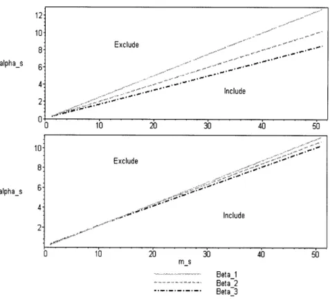
In Figure 3-1 we plot the threshold functions for a 3-period problem with rs = 1. The top graph has (A1, A2, A3) = (4,5,6) and the bottom one has (A1, A2, A3) =

(4.6, 4.8, 5.0) . The continuous lines are obtained by interpolating the function values for the integer points. In the bottom graph the threshold functions intersect around

ms m 13.

12 10 . Exclude .. . alpha_s 6 2

,.

..

,-.

Include

----

-- --- Beta

3

Figure 3-1: The threshold functions when A3 > A2 > A1.

3.3.4 The Index Policy

In this subsection we derive a heuristic index policy for the dynamic assortment

problem. This is done in two steps:

First Step: a Closed Form Approximation for the Single-Product Profit-to-go

* First, we impose At = A for all t, i.e. the shelf space opportunity cost is assumed

to be the same in all periods. The known arm in (3.6) is called in that case by Gittins a standard arm, and it follows from Proposition 4 that:

HtAs(m₈, s) = max rs , - A + En _t' ·(ms + ns, s as a s + 1)], 0}. (3.7) * Second, we implement a lookahead horizon of length one (see Bertsekas 2001). That is, in the recursive calculation of the expected profit at period t the

profit-Chapter 3. Model without Lost Sales

to-go of period t - 1 is approximated by the profit-to-go of stage 1. Formally, the profit-to-go Ht,_l(m, as) is thus approximated by:

ft

,s(ms as) = (t

1) max

A, 0

(3.8)

Substituting (3.8) in (3.7) and using [x]+ to denote the positive side of x, we

see that the optimal strategy at period t in the approximate problem depends on the sign of:

-Ax Ms a8 ,\ T~ ms + n

ii

Ai

as as +

Sfs O+1 1) En r, s b b

where b = IE[ns] = s and V[ns] = E[ns] ( )

rs a

/m

a

a

a

(3.9)

The second equality above is obtained through direct algebraic manipulation (similar to the example on p.12 in Berry and Fristedt 1985).

* Third, as a negative binomial with parameters ms and a,(a + 1)-_{1, n is the}

sum of ms independent geometric random variables; we thus approximate ns by a normal distribution with the same mean and variance, which is asymptotically exact as ms increases by the Central Limit Theorem. This yields:

dMas(ms, a) ~ as m ((t-1). * '(bs) - bs) (3.10)

where 'I(z) = (x - z)q(x)dx is the loss function of a standard normal.

Since (z) is continuous, positive and strictly decreasing (cf. DeGroot 1970, p.