Acquisition and reconstruction methods for magnetic resonance imaging

(1)

Acquisition and Reconstruction Methods for

Magnetic Resonance Imaging

by

Itthi Chatnuntawech

B.S., Carnegie Mellon University (2011)

S.M., Massachusetts Institute of Technology (2013)

Submitted to the Department of Electrical Engineering and Computer Science in partial fulfillment of the requirements for the degree of

Doctor of Philosophy in Electrical Engineering and Computer Science at the

MASSACHUSETTS INSTITUTE OF TECHNOLOGY June 2016

c

Author . . . . Department of Electrical Engineering and Computer Science

March 31, 2016

Certified by. . . .

Elfar Adalsteinsson

Professor of Electrical Engineering and Computer Science

Professor, Institute for Medical Engineering and Science

Thesis Supervisor

Accepted by . . . . Leslie A. Kolodziejski Chairman, Department Committee on Graduate Students

(2)

(3)

Acquisition and Reconstruction Methods for Magnetic

Resonance Imaging

by

Itthi Chatnuntawech

Submitted to the Department of Electrical Engineering and Computer Science on March 31, 2016, in partial fulfillment of the

requirements for the degree of

Doctor of Philosophy in Electrical Engineering and Computer Science

Abstract

Magnetic Resonance Imaging (MRI) is a non-invasive medical imaging modality that has a wide range of applications in both diagnostic clinical imaging and medical research. MRI has progressively gained in importance in clinical use because of its ability to produce high quality images of soft tissue throughout the body without sub-jecting the patient to any ionizing radiation. In addition to exquisite anatomical de-tail obtained from the conventional MRI, complementary physiological information is also available through emerging specialized applications of MRI such as magnetic res-onance spectroscopic imaging, quantitative susceptibility mapping, functional MRI, and diffusion MRI.

Despite its great versatility, MRI is limited by the long time required to acquire the data needed to form an image. Since a typical MRI protocol consists of multiple scans of the same patient, the total scan time is commonly extended beyond half an hour. During the session, the patient must remain perfectly still within a tight and closed environment, raising difficulties for certain populations such as children and patients with claustrophobia. The long acquisition time of MRI not only reduces the availability of the MRI scanner, but also results in patient discomfort, which often leads to motion that degrades image quality. Therefore, reducing the acquisition time of MRI is a well-motivated problem.

This thesis proposes acquisition and reconstruction methods that increase the imaging efficiency of MRI and two of its emerging specialized applications, magnetic resonance spectroscopic imaging and quantitative susceptibility mapping. In partic-ular, each of the proposed methods increases the imaging efficiency by achieving at least one of two aims: reduction of total scan time and improved image quality by mitigating image artifacts, while minimizing reconstruction time.

Thesis Supervisor: Elfar Adalsteinsson

Title: Professor of Electrical Engineering and Computer Science Professor, Institute for Medical Engineering and Science

(4)

(5)

Acknowledgments

I am grateful to all the people who have been a part of my graduate student life at MIT. This thesis would not have been possible without their support and encourage-ment in all my endeavors.

First, I wish to express my sincerest gratitude to my advisor, Professor Elfar Adalsteinsson, for his mentorship and guidance; he has tremendously impacted my professional and personal development. I have been blessed with the fortune of having such an encouraging, patient, flexible, and brilliant mentor.

I would like to extend my gratitude to my thesis committee members. To Pro-fessor Kawin Setsompop: thank you for your invaluable suggestions and creative ideas during numerous brainstorming sessions. To Professor Jacob K. White: thank you for your helpful suggestions and perceptive insights during our thesis committee meetings.

I have been fortunate enough to cross paths with many great people in the Mag-netic Resonance Imaging Group: Obaidah Abuhashem, Berkin Bilgic, Divya S. Bo-lar, Audrey P. Fan, Shao Ying Huang, Eren Can Kizildag, Trina Kok, Adrian Martin, Patrick McDaniel, Paula Montesinos, Tally Portnoi, Jeffrey Stout, Arlene Wint, Felipe Yanez, and Filiz Yetisir. Thank you all for the stimulating and thoughtful discussions we have had, in addition to providing an enjoyable work environment over the past few years.

Special thanks to Berkin for his guidance and friendship. I am greatly indebted to him for his significant intellectual and moral support throughout my graduate student life. I have benefitted greatly from his experience and expertise. Without his technical guidance and enthusiastic encouragement, this thesis would not have been completed. Paula, thank you for the good memories that we have shared together not only in the U.S., but also in Europe. I cherish our friendship. Audrey, thank you for always taking good care of everyone in the lab. Shao Ying and Trina, thank you for our weekly jogging sessions and funny conversations. Jeff, thank you for our enjoyable daily conversations and intellectual discussions that we have had. Patrick,

(6)

thank you for all the interesting discussions on so many random topics, ranging from quantum mechanics to tropical fruits. Adrian, thank you for the contribution on the multi-contrast MRI project and for the time we spent playing soccer together. Eren, thank you for the stimulating discussions on signal processing, optimization, and probability theory. Arlene, thank you for helping me and the lab team on ensuring experiments and tasks run smoothly in our lab.

I have had the wonderful opportunity to interact with many members of the Athinoula A. Martinos Center for Biomedical imaging: Stephen F. Cauley, Borjan Gagoski, Christin Y. Sander, Jason Stockmann, Lawrence L. Wald, Huihui Ye, and Bo Zhao. I thank Steve for teaching me many useful mathematical techniques. I thank Borjan for helping me with the MRSI project and teaching me how to run an MRI scan. I thank Christin for being such a great TA when I formally learned MRI for the first time. I thank Jason for helping me with the table-top MRI scanners. I thank Larry, Huihui, and Bo for the discussions we have had during our MRF meetings.

I would like to thank the Madrid-MIT M+Vision fellows: Ian Butterworth, Carlos Castro, Shivang Dave, Nicholas Durr, Javier Gonzalez, and German Gonzalez. It has been fun interacting with all of you especially during our soccer and basketball games. I wish to thank my friends who have greatly enriched my journey through gradu-ate school at MIT: Kamphol Akkaravarawong, Virot Chiraphadhanakul, Pakpong Chirarattananon, Thiparat Chotibut, Ittinop Dumnernchanvanit, Pimkwan Jaru-Ampornpan, Laphonchai Jirachuphun, Supanat Kamtue, Kritkorn Karntikoon, Tha-nard Kurutach, Tarek Aziz Lahlou, Chris Lai, Bunyada Laoprapassorn, Pasin Ma-nurangsi, Weerachai Neeranartvong, Payut Pantawongdecha, Nipun Pitimanaaree, Anchisa Pongmanavuth, Suppasit Pradyawong, Apiradee Sanglimsuwan, Guolong Su, Supasorn Suwajanakorn, Anupong Tangpeerachaikul, Omer Tanovic, Aniwat Tiralap, Atikhun Unahalekhaka, and Nopphon Weeranoppanant. I am truly grateful for their companionship. Special thanks to Arm for the memories and everything that we have been through together. It has been fun playing soccer, snowboarding, performing in a band, and traveling to many places around the world together. Nop, thank you for being such a respectful and caring roommate. Tarek, thank you for the countless

(7)

hours spent on brainstorming and studying with me through classes and research discussions.

I wish to thank my friends in Thailand for their lifelong friendship. I feel privileged to have gotten to know all of you. Thank you for always being there for me and keeping me sane.

My deepest gratitude goes to my family. I am eternally thankful for my parents and my sister for their unconditional love and unwavering support.

(8)

(9)

List of Figures

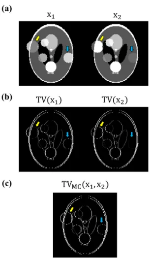
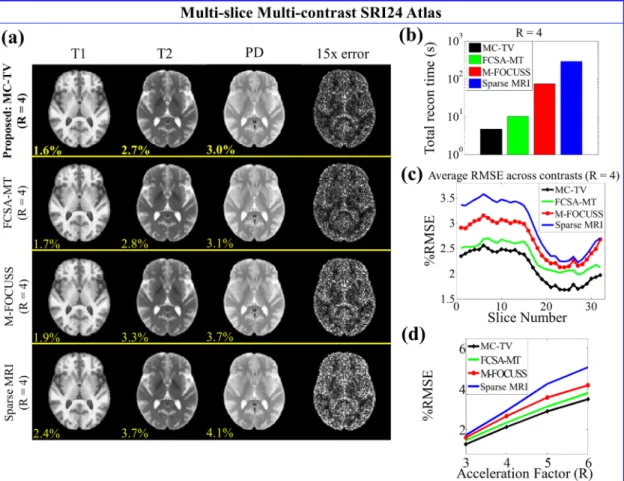
2.1 Total variation (TV) and multi-contrast total variation (MC-TV). (a) Simulated images with two different contrast settings. (b) Gradient images in the x direction used in TV regularization. (c) Square root sum-of-squares gradient image combining all the contrasts used in MC-TV regularization. . . 30 2.2 SRI24 atlas results at several acceleration factors. (a) Reconstructed

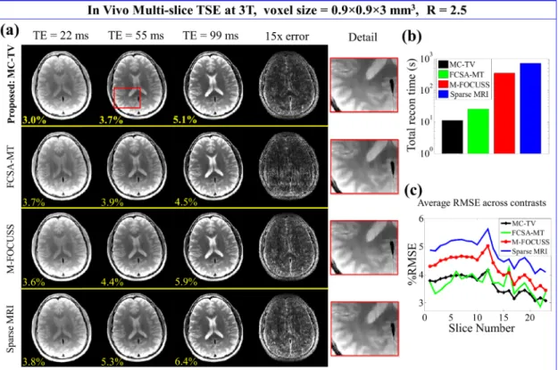
T1-, T2-, and PD-weighted images of slice three with corresponding RMSEs (yellow). The fourth column shows the sum-of-squares error across all contrasts. (b) Total reconstruction time of the 32-slice, 3-contrast data. (c) Average RMSE across all 3-contrasts of each slice. (d) Average RMSE across all slices and contrasts at R = 3, 4, 5, and 6. . 35 2.3 In vivo results at R = 2.5. (a) Reconstructed 3-contrast images of slice

nine with corresponding RMSEs (yellow). The fourth column shows the sum-of-squares error across all contrasts. The last column shows the zoomed-in views of the region indicated by the red box. (b) Total reconstruction time of the 23-slice, 3-contrast data. (c) Average RMSE across all contrasts of each slice. . . 36 2.4 Total variation (TV) and total generalized variation (TGV)

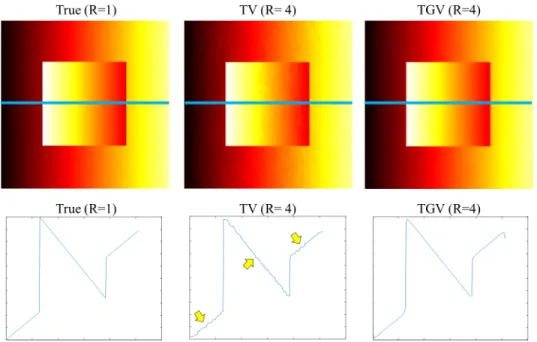
reconstruc-tions at an acceleration factor of four (R=4). The first row displays the reconstructed images. The second row shows a cross section of the region indicated by the blue line. The staircasing artifacts that are clearly visible in the TV reconstructed image (yellow arrows) are mitigated in the TGV reconstruction. . . 39

(12)

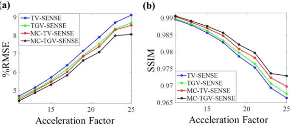
2.5 In vivo 3-contrast TSE results at different acceleration factors (1D un-dersampling). (a) RMSEs and (b) structural similarity (SSIM) indices of the reconstructed images averaged across all contrasts obtained from TV-SENSE, TGV-SENSE, MC-TV-SENSE, and MC-TGV-SENSE. . 45 2.6 In vivo 3-contrast TSE results at different acceleration factors (2D

un-dersampling). (a) RMSEs and (b) structural similarity (SSIM) indices of the reconstructed images averaged across all contrasts obtained from TV-SENSE, TGV-SENSE, MC-TV-SENSE, and MC-TGV-SENSE. . 45 2.7 Reconstructed 3-contrast TSE images at R = 5 (1D undersampling)

with corresponding RMSEs (yellow). . . 46 2.8 Reconstructed 3-contrast TSE images obtained from TV-SENSE (R

= 5) and MC-TGV-SENSE (R = 6) with their corresponding RMSEs (yellow). The zoomed-in views of the region indicated by the red box are displayed. The surface plots of the region indicated by the blue box are also shown with the height being proportional to the image intensity. . . 47 2.9 In vivo 4-contrast results at R = 5 (1D undersampling). (a) RMSEs

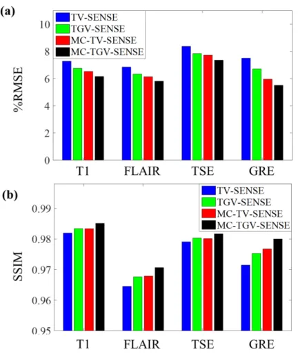
and (b) structural similarity (SSIM) indices of the reconstructed images obtained from TV-SENSE, TGV-SENSE, TV-SENSE, and MC-TGV-SENSE. . . 49 2.10 Reconstructed T1, FLAIR, TSE, and GRE images at R = 12 (2D

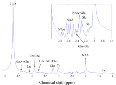
undersampling) with corresponding RMSEs (yellow). . . 50 3.1 A noise-free, lipid-free, water-suppressed synthetic MRS spectrum with

signal components from compounds observed in human brain tissues. This data set was simulated at three Tesla. The durations of the acqui-sition window were equal to 7.77 seconds with the bandwidth of 3.003 kHz. The chemical shift axis is displayed with decreasing frequency from left to right due to historical reasons. . . 56

(13)

3.2 (a) Two types of spiral-based k-space acquisition schemes: uniformly (top) and randomly (bottom) undersampled k-space acquisitions. The blue vertical lines represent the time at which a sample is acquired. (b) The projections of possible k-space trajectories onto the kx-ky plane.

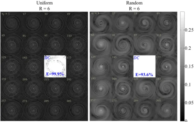
The projections obtained from the fully sampled, uniformly undersam-pled (R=3), and randomly undersamundersam-pled (R=3) acquisitions are shown from left to right, respectively. . . 59 3.3 An example of the point spread function (PSF) obtained from the

uni-form (left) and random (right) spiral-based k-space acquisition schemes at R=6. Each image is the absolute value of the PSF at a specific tem-poral frequency index, 𝑛𝑓 ∈ {1, 2, ..., 320}, with the brightest image

corresponding to the PSF at the zero temporal frequency (𝑛𝑓 = 161).

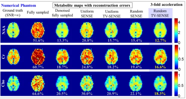
For the randomly undersampled k-space acquisition, the energy of the PSF contained at the zero temporal frequency is equal to 93.6%, com-pared to 99.9% for the uniformly undersampled k-space acquisition. . 61 3.4 Single-Slice Numerical Phantom. Reconstructed NAA, creatine, and

choline maps obtained from the six acquisition and reconstruction methods with a reduction in scan time by a factor of three. The cor-responding RMSE with respect to the MRSI data without noise is displayed under each reconstructed metabolite map. The acquisition parameters for different methods are summarized in Table 3.1. . . 69 3.5 Single-Slice Numerical Phantom. Reconstructed spectra obtained from

the fully sampled, denoised fully sampled, uniform TV-SENSE, and random TV-SENSE methods with a reduction in scan time by a factor of three. The ground truth (red) and reconstructed (blue) spectra were taken from the voxels indicated by the red dots in the structural image. 70

(14)

3.6 In Vivo Single-Slice MRSI. Reconstructed NAA, creatine, and choline maps obtained from the six acquisition and reconstruction methods with Tacq=1.44 minutes. The corresponding RMSE with respect to the

ground truth (Navg=50 and R=1) is displayed under each reconstructed

metabolite map. The acquisition parameters for different methods are summarized in Table 3.2. . . 71 3.7 In Vivo Single-Slice MRSI. Reconstructed NAA, creatine, and choline

maps obtained from the six acquisition and reconstruction methods with Tacq=42 seconds. The corresponding RMSE with respect to the

ground truth (Navg=50 and R=1) is displayed under each reconstructed

metabolite map. The acquisition parameters for different methods are summarized in Table 3.3. . . 71 3.8 In Vivo Single-Slice MRSI. Reconstructed spectra obtained from the

fully sampled, denoised fully sampled, uniform TV-SENSE, and ran-dom TV-SENSE methods with Tacq=1.44 minutes. The ground truth

(red) and reconstructed (blue) spectra were taken from the voxels in-dicated by the red dots in the structural GRE image. . . 72 3.9 In Vivo Single-Slice MRSI. Reconstructed spectra obtained from the

fully sampled, denoised fully sampled, uniform TV-SENSE, and ran-dom TV-SENSE methods with Tacq=42 seconds. The ground truth

(red) and reconstructed (blue) spectra were taken from the voxels in-dicated by the red dots in the structural GRE image. . . 73

(15)

3.10 In Vivo Single-Slice MRSI. (a) Reconstructed NAA maps obtained from the 18-average fully sampled data and random TV-SENSE construction. The corresponding acquisition time and RMSE with re-spect to the ground truth (Navg=50 and R=1) are displayed above and

below each reconstructed NAA map, respectively. By using random TV-SENSE, an acceleration factor of 4.5 was achievable with the same quality as the fully sampled data, as measured by the RMSE of the reconstructed NAA map. (b) The reconstructed spectra of the in vivo data obtained from the fully sampled and random TV-SENSE meth-ods. The ground truth (red) and reconstructed (blue) spectra were taken from the voxels indicated by the red dots in the structural GRE image. . . 75 3.11 In Vivo 3D-MRSI. (a) Reconstructed NAA, creatine, and choline maps

obtained from uniform TV-SENSE and random TV-SENSE with Tacq=1.70

minutes. The corresponding RMSE with respect to the ground truth (Navg=4 and R=1) is displayed under each reconstructed metabolite

map. The ground truth (red) and reconstructed (blue) spectra were taken from the voxels indicated by the red dots in the structural im-age. (b) Reconstructed NAA maps and spectra obtained from the single-average, fully sampled data and random TV-SENSE reconstruc-tion with R=4. The corresponding acquisireconstruc-tion time and RMSE with respect to the ground truth are displayed above and below each recon-structed NAA map, respectively. . . 76 3.12 In Vivo 3D-MRSI. Reconstructed NAA, creatine, and choline maps of

two consecutive slices obtained using random TV-SENSE with R = 4 (Tacq=1.27 minutes). . . 77

4.1 The pipeline of the proposed rapid, automated and phase-sensitive coil sensitivity estimation for Wave-CAIPI. . . 100

(16)

4.2 Multi-Echo Wave-CAIPI. The unwrapped phase images were normal-ized by their TEs and averaged for improved SNR. The resulting com-bined phase was then processed by the QSM algorithms. . . 100 4.3 Duke Brain Phantom. The reconstructed magnetic susceptibility maps

obtained from six different QSM algorithms with their corresponding RMSEs. . . 103 4.4 Duke Brain Phantom. The difference maps between the reconstructed

magnetic susceptibility maps and the underlying tissue susceptibility distribution with the corresponding RMSEs. . . 104 4.5 Numerical Brain Phantom. The reconstructed magnetic susceptibility

maps obtained from six different QSM algorithms with their corre-sponding RMSEs. . . 105 4.6 Numerical Brain Phantom. The difference maps between the

recon-structed magnetic susceptibility maps and the underlying tissue sus-ceptibility distribution with the corresponding RMSEs. . . 106 4.7 Numerical Brain Phantom. RMSEs of the reconstructed magnetic

sus-ceptibility maps obtained from six different methods. . . 106 4.8 3D-EPI. The reconstructed magnetic susceptibility maps obtained from

the multi-step (14 SMV kernels) and single-step (5 SMV kernels) meth-ods. . . 107 4.9 3D-EPI. The reconstructed magnetic susceptibility maps obtained from

six different QSM algorithms with five SMV kernels. . . 108 4.10 Multi-Echo Wave-CAIPI. The reconstructed magnetic susceptibility

maps obtained from six different QSM algorithms. . . 109 4.11 High-Resolution Wave-CAIPI at 7 Tesla. The reconstructed magnetic

susceptibility maps obtained from six different QSM algorithms. . . . 110 4.12 In vivo data sets. The difference maps between the two proposed

(17)

List of Tables

2.1 In Vivo 4-Contrast Data: Acquisition Parameters . . . 44 3.1 Single-Slice Numerical Phantom. Acquisition parameters with the

cor-responding RMSEs of the reconstructed NAA, creatine, and choline maps. . . 65 3.2 In Vivo Single-Slice MRSI with Matched Acquisition Time.

Acqui-sition parameters (Tacq=1.44 min) with the corresponding RMSEs of

the reconstructed NAA, creatine, and choline maps. . . 66 3.3 In Vivo Single-Slice MRSI with Matched Acquisition Time.

Acqui-sition parameters (Tacq=42 s) with the corresponding RMSEs of the

reconstructed NAA, creatine, and choline maps. . . 66 4.1 Reconstruction parameters of each QSM method. For Numerical Brain

Phantom, the reconstruction parameters were reported for the case where we used 5 SMV kernels for all the methods. For 3D-EPI, the reconstruction parameters were reported for the case where we used 5 SMV kernels for the single-step methods and 14 SMV kernels for the multi-step methods. . . 96 4.2 Reconstruction time of each QSM method. For Numerical Brain

Phan-tom, the reconstruction times were reported for the case where we used 5 SMV kernels for all the methods. For 3D-EPI, the reconstruction times were reported for the case where we used 5 SMV kernels for the single-step methods and 14 SMV kernels for the multi-step methods. . 101

(18)

(19)

Chapter 1 Introduction

Magnetic Resonance Imaging (MRI) is a non-invasive medical imaging modality that has a wide range of applications in both diagnostic clinical imaging and medical research. MRI has progressively gained in importance in clinical use because of its ability to produce high quality images of soft tissue throughout the body without sub-jecting the patient to any ionizing radiation. In addition to exquisite anatomical de-tail obtained from the conventional MRI, complementary physiological information is also available through emerging specialized applications of MRI such as magnetic res-onance spectroscopic imaging, quantitative susceptibility mapping, functional MRI, and diffusion MRI.

Despite its great versatility, MRI is limited by the long time required to acquire the data needed to form an image. Since a typical MRI protocol consists of multiple scans of the same patient, the total scan time is commonly extended beyond half an hour. During the session, the patient must remain perfectly still within a tight and closed environment, raising difficulties for certain populations such as children and patients with claustrophobia. The long acquisition time of MRI not only reduces the availability of the MRI scanner, but also results in patient discomfort, which often leads to motion that degrades image quality. Therefore, reducing the acquisition time of MRI is a well-motivated problem.

Main efforts in reducing the acquisition time of MRI have recently centered upon using parallel imaging, compressed sensing, and the combination of both techniques.

(20)

These techniques accelerate the data acquisition process by reducing the amount of acquired data, and the underlying images are then estimated from the undersampled measurements by solving a mathematical optimization problem. Parallel imaging collects samples of nearly distinct information content simultaneously using multi-ple receiver channels that are sensitive to different parts of the object being imaged. The ambiguity due to undersampling artifacts are resolved by exploiting different non-uniform sensitivities of the receiver channels [1–3]. Instead of using the encod-ing power of multiple receiver channels, compressed sensencod-ing estimates the underlyencod-ing data from undersampled measurements by exploiting data redundancy [4, 5]. It has been demonstrated that MRI data are approximately sparse or compressible in some transform domains, so the underlying information can be recovered from many fewer number of measurements than traditionally considered necessary by solving a regular-ized mathematical optimization problem that imposes transform sparsity constraints [6].

This thesis proposes acquisition and reconstruction methods that increase the imaging efficiency of MRI and two of its emerging specialized applications, magnetic resonance spectroscopic imaging and quantitative susceptibility mapping. In partic-ular, each of the proposed methods increases the imaging efficiency by achieving at least one of two aims: reduction of total acquisition time and improved image quality by mitigating image artifacts, while minimizing reconstruction time.

1.1 Outline

The detailed structure of this thesis is as follows.

Chapter 2 focuses on multi-contrast MRI, which is routinely included in a stan-dard clinical MRI protocol. Multi-contrast MRI acquires data from the same region of interest multiple times with different contrast preparations, providing complemen-tary diagnostic information, however, with prolonged scan time. This chapter pro-poses two joint reconstruction methods for accelerated multi-contrast MRI: one for the single-channel case and one for the multi-channel case. Compared to the

(21)

meth-ods that reconstruct each image contrast independently of each other, the proposed joint reconstruction methods improve the reconstruction quality by exploiting not only the sparsity of each image contrast in a transform domain, but also the shared information among the contrast images. In the single-channel case, the multi-contrast images are reconstructed from the undersampled k-space data by solving an optimization problem with vectorial total variation (TV) regularization [7–9]. A reconstruction algorithm that efficiently solves the regularized optimization problem using simple analytical update rules is developed based on the alternating direction method of multipliers (ADMM) [10–18] and special properties of circulant matrices. In the multi-channel case, a more advanced reconstruction method is developed by incorporating the encoding power of multiple receive coils [2, 19] and vectorial total generalized variation (TGV) regularization [20, 21] into the proposed single-channel multi-contrast reconstruction method to further improve the image reconstruction quality. An efficient reconstruction algorithm for the multi-channel case is also devel-oped based on ADMM.

Chapter 3 is devoted to the discussion of 1H Magnetic Resonance Spectroscopic

Imaging (1_{H-MRSI). As opposed to conventional MRI, which derives its signal from}

hydrogen nuclei in water, 1H-MRSI acquires the magnetic resonance signal from

hy-drogen nuclei in other chemical components including various metabolites in the body. Since the molecular concentrations of the metabolites are typically at least 10,000 times lower than water, 1_{H-MRSI suffers from low signal-to-noise ratio (SNR).}

An-other technical challenge of 1H-MRSI is the long acquisition time required to collect

all necessary information. Because 1_{H-MRSI encodes the spectral dimension(s) in}

addition to the spatial dimensions encoded in the conventional MRI, the total acqui-sition time of1_{H-MRSI becomes much longer than that of MRI. Despite the challenges}

posed by the low SNR and long acquisition time, the development of1H-MRSI is

moti-vated by the desire to directly observe signal sources other than water, which provides important physiological and biochemical information. This chapter proposes an ac-quisition and reconstruction method to accelerate 1_{H-MRSI. The proposed method}

(22)

both spatial and spectral domains using spirals with different radii. The underlying

1H-MRSI data are estimated from the undersampled k-space data using the

sensi-tivity encoding technique (SENSE) [2, 19] with total variation regularization. The proposed acquisition and reconstruction method benefits from the efficient sampling scheme, increased randomness in sampling patterns, compressed sensing, and parallel imaging.

Chapter 4 focuses on Quantitative Susceptibility Mapping (QSM), which is an emerging specialized application of MRI that aims to estimate the underlying tis-sue magnetic susceptibility distribution from the phase images derived from gradient echo (GRE) acquisitions. The underlying tissue magnetic susceptibility is useful for various applications including chemical identification, and quantification of venous oxygen saturation (SvO2) and specific biomarkers such as gadolinium and iron.

Con-ventional QSM methods involve successive application of multiple post-processing steps consisting of phase unwrapping, removal of phase contributions from background sources, and solving an ill-posed inverse problem relating the unwrapped tissue phase to the underlying tissue magnetic susceptibility distribution. It has recently been demonstrated that combining the post-processing steps into one single step prevents potential error propagation through successive operations and hence improves the re-construction accuracy of QSM [22–26]. This chapter proposes new single-step QSM methods that benefit from the three components: (i) the single-step processing that prevents potential error propagation normally encountered in multi-step QSM meth-ods, (ii) multiple spherical mean value kernels that permit high fidelity background phase removal, and (iii) TV or TGV regularization that imposes prior information on the solution. Fast solvers for the proposed methods, which enable simple analyt-ical solutions to all of the optimization steps, are also developed based on ADMM, variable splitting, and special structures of the matrices.

Chapter 5 provides some potential extensions of the methods developed in this thesis.

(23)

1.2 Bibliographical Notes

The single-channel multi-contrast MRI section of Chapter 2 appears in:

∙ I. Chatnuntawech, B. Bilgic, A. Martin, K. Setsompop, E. Adalsteinsson. Fast Reconstruction for Accelerated Multi-Slice Multi-Contrast MRI. In Proc. IEEE International Symposium on Biomedical Imaging, pp. 335-338, 2015. ∙ I. Chatnuntawech, B. Bilgic, A. Martin, K. Setsompop, E. Adalsteinsson. A

Fast Reconstruction Algorithm for Accelerated Multi-Contrast MRI. In Proc. International Society for Magnetic Resonance in Medicine 23rd Scientific Meet-ing, p. 3710, 2015.

The multi-channel multi-contrast MRI section of Chapter 2 has been developed with Adrian Martin Fernandez, a Ph.D. student at Universidad Rey Juan Carlos, Mostoles, Madrid, Spain, with equal contributions. Therefore, the contents will also appear in his Ph.D. thesis. Parts of this section have been submitted for publication:

∙ I. Chatnuntawech†_{, A. Martin}†_{, B. Bilgic, K. Setsompop, E. Adalsteinsson, E.}

Schiavi. Vectorial Total Generalized Variation for Accelerated Multi-Channel Multi-Contrast MRI. †_{The authors contributed equally to this work.}

Parts of Chapter 3 appear in:

∙ I. Chatnuntawech, B. A. Gagoski, B. Bilgic, S. F. Cauley, K. Setsompop, E. Adalsteinsson. Accelerated 1H MRSI Using Randomly Undersampled

Spiral-Based k-Space Trajectories. Magnetic Resonance in Medicine, vol. 74, pp. 13-24, 2015.

∙ I. Chatnuntawech, B. A. Gagoski, B. Bilgic, S. F. Cauley, P. E. Grant, K. Set-sompop, E. Adalsteinsson. Accelerated MRSI Using Randomly Undersampled Spiral-Based k-Space Trajectories. In Proc. International Society for Magnetic Resonance in Medicine 22nd Scientific Meeting, p. 3719, 2014.

(24)

∙ I. Chatnuntawech, P. McDaniel, S. F. Cauley, B. A. Gagoski, C. Langkam-mer, A. Martin, P. E. Grant, L. L. Wald, K. Setsompop, E. Adalsteinsson, B. Bilgic. TGV-Regularized Single-Step Quantitative Susceptibility Mapping. In Proc. International Society for Magnetic Resonance in Medicine 24th Scientific Meeting, 2016.

and have been submitted for publication:

∙ I. Chatnuntawech, P. McDaniel, S. F. Cauley, B. A. Gagoski, C. Langkammer, A. Martin, P. E. Grant, L. L. Wald, K. Setsompop, E. Adalsteinsson, B. Bilgic. TGV-Regularized Single-Step Quantitative Susceptibility Mapping.

1.3 Other Peer-Reviewed Publications as a Doctoral

Student at MIT

∙ B. Bilgic, I. Chatnuntawech, C. Langkammer, K. Setsompop. Sparse Meth-ods for Quantitative Susceptibility Mapping. In Proc. SPIE Wavelets and Sparsity XVI, vol. 9597, pp. 959711-1-10, 2015.

∙ A. Martin, I. Chatnuntawech, B. Bilgic, K. Setsompop, E. Adalsteinsson, E. Schiavi. Total Generalized Variation Based Multi-Contrast Magnetic Resonance Image Reconstruction. In Proc. XXIII CEDYA - XIII CMA, p. 135. Cadiz, Spain, 2015.

∙ A. Martin, I. Chatnuntawech, B. Bilgic, K. Setsompop, E. Adalsteinsson, E. Schiavi. Total Generalized Variation Based Joint Multi-Contrast, Parallel Imaging Reconstruction of Undersampled k-space Data. In Proc. International Society for Magnetic Resonance in Medicine 22nd Scientific Meeting, p. 80, 2015.

∙ B. Gagoski, H. Ye, S.F. Cauley, H. Bhat, K. Setsompop, I. Chatnuntawech, A. Martin, Y. Jiang, M. Griswold, E. Adalsteinsson, P.E. Grant, L.L. Wald.

(25)

Proc. International Society for Magnetic Resonance in Medicine 22nd Scientific Meeting, p. 3429, 2015.

∙ K. Setsompop, B. Bilgic, A. Nummenmaa, Q. Fan, S.F. Cauley, S. Huang, I. Chatnuntawech, Y. Rathi, T. Witzel, L.L. Wald. Slice Dithered Enhanced Resolution Simultaneous Multislice (SLIDER-SMS) for High Resolution (700 um) Diffusion Imaging of the Human Brain. In Proc. International Society for Magnetic Resonance in Medicine 22nd Scientific Meeting, p. 339, 2015.

∙ T. Chang, P. Shi, J.D. Steinmeyer, I. Chatnuntawech, P. Tillberg, K.T. Love, P.M. Eimon, D.G. Anderson, M.F. Yanik. Organ-Targeted High-Throughput In Vivo Biologics Screen Identifies Materials for RNA Delivery. Integrative Biology, vol. 6, pp. 926-934, 2014.

∙ B. Bilgic, I. Chatnuntawech, A.P. Fan, K. Setsompop, S.F. Cauley, L.L. Wald, E. Adalsteinsson. Fast Image Reconstruction with L2-Regularization. Journal of Magnetic Resonance Imaging, vol. 40, pp. 181-191, 2013.

∙ B. Bilgic, I. Chatnuntawech, K. Setsompop, S.F. Cauley, L.L. Wald, E. Adal-steinsson. Fast Dictionary-Based Reconstruction for Diffusion Spectrum Imag-ing. IEEE Transactions on Medical Imaging, vol. 32, no. 11, pp. 2022-2033, 2013.

∙ B. Bilgic, I. Chatnuntawech, A.P. Fan, E. Adalsteinsson. Regularized QSM in Seconds. In Proc. International Society for Magnetic Resonance in Medicine 21st Scientific Meeting, p. 168, 2013.

∙ B. Bilgic, I. Chatnuntawech, K. Setsompop, S.F. Cauley, L.L. Wald, E. Adal-steinsson. Fast Regularized Reconstruction Tools for QSM and DSI. In Proc. International Society for Magnetic Resonance in Medicine Workshop on Data Sampling and Image Reconstruction, 2013.

∙ I. Chatnuntawech, B. Bilgic, E. Adalsteinsson; Undersampled Spectroscopic Imaging with Model-based Reconstruction. In Proc. International Society for

(26)

Magnetic Resonance in Medicine 21st Scientific Meeting, p. 3960, 2013.

∙ I. Chatnuntawech, B. Bilgic, B. Gagoski, T. Kok, A.P. Fan, E. Adalsteinsson. Metabolite Map Estimation from Undersampled Spectroscopic Imaging Data using N-Compartment Model. In Proc. International Society for Magnetic Resonance in Medicine 21st Scientific Meeting, p. 3968, 2013.

∙ B. Bilgic, I. Chatnuntawech, K. Setsompop, S.F. Cauley, L.L. Wald, E. Adal-steinsson. Fast DSI Reconstruction with Trained Dictionaries. In Proc. Inter-national Society for Magnetic Resonance in Medicine 21st Scientific Meeting, p. 58, 2013.

∙ S.F. Cauley, O.A. Abuhashem, B. Bilgic, I. Chatnuntawech, J. Cohen-Adad, K. Setsompop, L.L. Wald, E. Adalsteinsson. Low-Rank Basis Smoothing for the Denoising of Diffusion Weighted Images. In Proc. International Society for Magnetic Resonance in Medicine 21st Scientific Meeting, p. 2077, 2013.

(27)

Chapter 2 Accelerated Multi-Contrast Magnetic

Resonance Imaging

In clinical applications of magnetic resonance imaging (MRI), data from the same re-gion of interest are routinely acquired with different contrast preparations. A standard clinical multi-contrast MRI protocol typically includes T1-weighted and T2-weighted images. T1-weighted images are useful for various applications including the identifi-cation of adipose tissue [27–29] and the measurement of the volume and thickness of the cerebral cortex, which provides valuable information on both normal development and neurodegenerative disorders [30, 31]. T2-weighted images are useful for charac-terizing abnormalities such as edema, tumors, inflammation, and white matter lesions [32–34]. The fluid-attenuated inversion recovery (FLAIR) pulse sequence is also used in clinical routine to null fluids, providing us with another type of image contrast in addition to the T1 and T2 contrasts [35]. By using the FLAIR pulse sequence, the periventricular hyperintense lesions such as multiple sclerosis (MS) plaques become more noticeable because cerebrospinal fluid (CSF) is suppressed [36–39].

The complementary diagnostic information obtained from different contrast prepa-rations comes at a cost of prolonged acquisition time, which not only reduces the availability of the MRI scanner, but also increases patient discomfort. This chapter presents two approaches based on compressed sensing [4, 5] and parallel imaging [2, 19] for reducing the total acquisition time of multi-contrast MRI. The chapter is divided

(28)

into two major sections: single-channel contrast MRI and channel multi-contrast MRI. The first section presents an efficient algorithm for jointly reconstruct-ing sreconstruct-ingle-channel multi-contrast data from undersampled k-space data. The second section develops a reconstruction method that combines both compressed sensing and parallel imaging to improve the reconstruction accuracy of accelerated multi-channel multi-contrast MRI.

2.1 Single-Channel Multi-Contrast MRI

Compressed sensing has successfully been used to accelerate the data acquisition pro-cess of MRI and multi-contrast MRI by reducing the number of acquired k-space sam-ples. One way to reconstruct the underlying images from the undersampled k-space data is to solve a regularized optimization problem that imposes prior knowledge on each image contrast independently of each other [6]. To further improve the recon-struction accuracy of single-channel multi-contrast MRI, several joint reconrecon-structions that make use of shared features among the multi-contrast images have been devel-oped [40–44]. The idea of using shared information has also been used in several imaging applications including color photography [9, 21], diffusion MRI [45], spec-tral computed tomography [46], and a combination of positron emission tomography (PET) and MRI [47].

It was demonstrated that the joint reconstructions that imposed group sparsity in the Wavelet domain [40] or finite difference domain [41] resulted in more accurate ac-celerated multi-contrast MRI than the conventional contrast-by-contrast reconstruc-tion [6]. In [42], a reconstrucreconstruc-tion method based on joint Bayesian compressed sens-ing (JBCS) was developed to further improve the reconstruction quality compared to the joint multi-contrast reconstruction that imposed group sparsity in the finite difference domain implemented using Multiple measurement vectors FOCal Under-determined System Solver (M-FOCUSS) [48]. The recently developed method called FCSA-MT uses a combination of the group Wavelet sparsity and joint total variation (TV) as a regularizer [43, 44] and efficiently reconstructs the multi-contrast data

(29)

us-ing a combination of Fast Composite Splittus-ing Algorithm (FCSA) and Fast Iterative Shrinkage-Thresholding Algorithm (FISTA). It was shown that FCSA-MT gave bet-ter reconstruction quality with fasbet-ter reconstruction compared to other conventional methods including JBCS.

In this section, an efficient algorithm is developed based on the alternating di-rection method of multipliers (ADMM) [10–18] and properties of circulant matrices to reduce the processing time of the joint multi-contrast reconstruction that uses joint total variation regularization, while maintaining equivalent reconstruction qual-ity compared to FCSA-MT.

2.1.1 Theory

Problem Formulation

The following optimization problem with multi-contrast total variation (MC-TV) regularization is solved to reconstruct the three-dimensional data of size 𝑁𝑥× 𝑁𝑦× 𝑁𝑧

voxels with 𝐿 different contrasts minimize 𝑥1,...,𝑥𝐿 1 2 𝐿 ∑︁ 𝑙=1 ‖𝑀𝑙𝐹 𝑥𝑙− 𝑦𝑙‖22+ 𝜆𝑇 𝑉𝑀 𝐶(𝑥1, ..., 𝑥𝐿), (2.1)

where 𝑥𝑙is the vectorized image of the 𝑙th contrast, 𝐹 is the fully sampled 3D discrete

Fourier transform operator, 𝑀𝑙 is the 3D undersampling mask for the 𝑙th image

con-trast, 𝑦𝑙is the observed 3D k-space data on a Cartesian grid, and 𝜆 is a regularization

parameter.

The first term of Eq. (2.1) is the data consistency term, which ensures that the reconstructed multi-contrast images are consistent with the observed data in k-space. The second term is the MC-TV regularization term enforcing joint sparsity of the multi-contrast images in the gradient domain. MC-TV regularization is defined as follows 𝑇 𝑉𝑀 𝐶(𝑥1, ..., 𝑥𝐿) = ‖𝐺𝑋‖2,1 = ∑︁ 𝑛 √︃ ∑︁ 𝑙 |(𝐺𝑋)𝑛,𝑙|2, (2.2)

(30)

Figure 2.1: Total variation (TV) and multi-contrast total variation (MC-TV). (a) Simulated images with two different contrast settings. (b) Gradient images in the x direction used in TV regularization. (c) Square root sum-of-squares gradient image combining all the contrasts used in MC-TV regularization.

where 𝑋 = [𝑥1, ..., 𝑥𝐿], ‖ · ‖2,1 is the ℓ2,1-mixed norm, 𝐺 is the 3D gradient operator

discretized using finite differences, and (𝐺𝑋)𝑛,𝑙 represents the element at the 𝑛th row

and 𝑙th _{column of 𝐺𝑋.}

Figure 2.1 shows two simulated images with different contrast preparations and their gradients in the x direction, demonstrating the differences between TV and MC-TV regularizations. On the one hand, the contrast-by-contrast MC-TV imposes sparsity on the gradient images of each contrast setting separately (Figure 2.1b)

𝑇 𝑉 (𝑥1, ..., 𝑥𝐿) =

∑︁

𝑇 𝑉 (𝑥𝑙) =

∑︁

(31)

On the other hand, MC-TV imposes sparsity on the square root sum-of-squares gra-dient images combining all the contrasts (Figure 2.1c and Eq. (2.2)). As shown in Figure 2.1b, each gradient image has non-uniform gradient intensities. By enforcing sparsity on it, the spatial locations of the gradient image with high intensities are well-preserved, while the spatial locations with low intensities could be eliminated. In other words, the strong edges in the image are preserved, whereas the weak edges could be attenuated or completely eliminated. In this specific example, by using the contrast-by-contrast TV regularization, the edges in the first image, x1, indicated by

the yellow arrow will likely be attenuated in the reconstruction process. Similarly, the edges in the second image, x2, indicated by the blue arrow could be lost.

Assum-ing that there is no motion, the locations of the edges in the images with different contrast settings should be the same. Consequently, enforcing sparsity on the square root sum-of-squares gradient image (Figure 2.1c) as done in the multi-contrast TV regularization prevents the elimination of weak edges because the strong edges from all image contrasts are included in this image.

Implementation

To efficiently solve the optimization problem shown in Eq. (2.1), the additional variable 𝑍 = [𝑧1, 𝑧2, ..., 𝑧𝐿]and its corresponding consensus constraint are introduced

minimize 𝑋,𝑍 1 2 𝐿 ∑︁ 𝑙=1 ‖𝑀𝑙𝐹 𝑥𝑙− 𝑦𝑙‖22 + 𝜆‖𝑍‖2,1 subject to 𝐺𝑋 = 𝑍. (2.4) The scaled form of ADMM applied to Eq. (2.4) can be expressed as

𝑋𝑘+1 :=argmin 𝑋 1 2 𝐿 ∑︁ 𝑙=1 ‖𝑀𝑙𝐹 𝑥𝑙− 𝑦𝑙‖22+ 𝜇 2‖𝐺𝑋 − (𝑍 𝑘_{− 𝑆}𝑘_)‖2 𝐹 (2.5) 𝑍𝑘+1 :=argmin 𝑍 1 2‖𝑍 − (𝐺𝑋 𝑘+1_{+ 𝑆}𝑘_)‖2 𝐹 + 𝜆 𝜇‖𝑍‖2,1 (2.6) 𝑆𝑘+1 := 𝑆𝑘+ 𝐺𝑋𝑘+1− 𝑍𝑘+1_, _(2.7)

(32)

where 𝑆 is the scaled dual variable, 𝜇 is the augmented Lagrangian parameter, ‖ · ‖𝐹

is the Frobenius norm, and the superscript is the iteration counter.

By rewriting the Frobenius norm in Eq. (2.5) as a summation of the ℓ2 norms, we

can reconstruct each image contrast 𝑥𝑙 independently

𝑥𝑘+1_𝑙 :=argmin 𝑥𝑙 1 2‖𝑀𝑙𝐹 𝑥𝑙− 𝑦𝑙‖ 2 2+ 𝜇 2‖𝐺𝑥𝑙− (𝑧 𝑘 𝑙 − 𝑠 𝑘 𝑙)‖ 2 2. (2.8)

Setting the gradient with respect to 𝑥𝑙 to zero gives

(𝐹*𝑀_𝑙*𝑀𝑙𝐹 + 𝜇𝐺*𝐺)𝑥𝑙 = 𝐹*𝑀𝑙*𝑦𝑙+ 𝜇𝐺*(𝑧𝑙𝑘− 𝑠 𝑘

𝑙), (2.9)

where * _{denotes the Hermitian transpose. Diagonalizing the finite difference matrix}

by the discrete Fourier transform (i.e., 𝐺 = 𝐹−1_𝐸𝐹_{), the following analytical update}

for 𝑥𝑙 is obtained

𝑥𝑘+1_𝑙 := 𝐹−1[︀(𝑀_𝑙*𝑀𝑙+ 𝜇𝐸*𝐸)−1(𝑀𝑙*𝑦𝑙+ 𝜇𝐸*𝐹 (𝑧𝑙𝑘− 𝑠 𝑘

𝑙))]︀ . (2.10)

In Eq. (2.10), the terms (𝑀*

𝑙𝑀𝑙+ 𝜇𝐸*𝐸)−1 and 𝑀𝑙*𝑦𝑙can be pre-computed to further

speed up the reconstruction process. Since 𝑀*

𝑙𝑀𝑙+ 𝜇𝐸*𝐸 is a diagonal matrix, it is

straightforward to compute its inverse. Consequently, 𝑥𝑙 can be updated using only

two FFT operations and a few matrix additions and multiplications.

The 𝑍-update step in Eq. (2.6) can be performed easily using the voxel-wise vector soft-thresholding operator

𝑍_(𝑛)𝑘+1 := (𝐺𝑋𝑘+1+ 𝑆𝑘)(𝑛)∘ max (︂ 1 − 𝜆/𝜇 ‖(𝐺𝑋𝑘+1_{+ 𝑆}𝑘₎ (𝑛)‖2 , 0 )︂ , (2.11)

where ∘ denotes the Hadamard product, and the subscript in parenthesis is the voxel label.

In summary, the proposed optimization problem with multi-contrast TV regular-ization is solved by iterating Eqs. (2.7), (2.10), and (2.11) until convergence.

(33)

2.1.2 Methods

We compared the performance of the proposed method (MC-TV) to the previously proposed FCSA-MT [43, 44] and M-FOCUSS [48] algorithms for joint multi-contrast reconstruction, and Sparse MRI [6] for contrast-by-contrast compressed sensing using the SRI24 atlas [49] and in vivo data. The reconstruction algorithms were imple-mented in MATLAB (with FCSA-MT provided by the lead author of [43, 44]) and run on a machine with 16 Intel Xeon E5-2670 processors and 128 GB of memory. All slices were reconstructed together for MC-TV, M-FOCUSS, and Sparse MRI, whereas each slice was reconstructed independently for FCSA-MT as done in their implemen-tation. For MC-TV, FCSA-MT, and Sparse MRI, we selected a regularization param-eter that yielded the smallest normalized root-mean-square error (RMSE) as defined by RMSE = 100×‖̂︀𝑥−𝑥‖2/‖𝑥‖2 where 𝑥 is the fully sampled data, and𝑥̂︀is the recon-structed data. For all the methods, whenever the fully sampled data were real-valued, RMSEs were computed based on the real part of the reconstructed data. The stopping criterion for all methods was that the relative change in %RMSE between consecutive iterations is less than 1%, i.e. when 100 × ‖RMSE𝑘+1 ₋_RMSE𝑘_‖

2/‖RMSE𝑘‖2 < 1

where RMSE𝑘 _{is the normalized %RMSE at iteration 𝑘.}

Multi-Slice Multi-Contrast SRI24 Atlas

The 32-slice, 3-contrast data were extracted from the SRI24 atlas with a field-of-view (FOV) of 20 cm × 20 cm, which resulted in a matrix size of 108 × 108. T1-weighted images were generated using the IR-prep Spoiled Gradient Recalled (SPGR) sequence with repetition time (TR) = 6.5 ms, and echo time (TE) = 1.54 ms. T2-weighted and proton density (PD) weighted images were simulated using the dual-echo fast spin echo (FSE) sequence with TR = 10 s, and TEs = 98 ms and 14 ms, respectively. The k-space data were undersampled along the two phase-encoding directions, kx

and ky (z is the readout direction), using 2D pseudo-random variable-density masks

[6] with acceleration factors between three and six (R = 3, 4, 5, and 6). Different undersampling masks were used for different contrast settings.

(34)

In Vivo Multi-Slice Multi-Contrast Data

A dataset with three different contrasts and 23 slices was acquired fully sampled from a healthy volunteer with the institutional review board approval and informed consent at three Tesla in 4:20 minutes using the turbo spin-echo (TSE) acquisition with the following parameters: voxel size = 0.9 × 0.9 × 3.0 mm3_{, in-plane field-of-view (FOV)}

= 22 cm × 22 cm, TEs = 22/55/99 ms, and TR = 4 s. The fully sampled 32-channel data were combined and reconstructed. The resulting coil combined k-space data were retrospectively undersampled along the phase encoding direction (kx) with

R = 2.5. Different undersampling masks were used for different slices and contrasts. Although a single regularization parameter 𝜆 was assigned to the regularization term, the effective penalty on the gradient along each direction was adjusted to account for the anisotropic voxel size.

2.1.3 Results

Figure 2.2 presents the reconstruction results for the SRI24 atlas at several accelera-tion factors. Figure 2.3 shows the in vivo results with R = 2.5. The joint reconstruc-tions were more successful at preserving the edges and removing the undersampling artifacts. With the contrast-by-contrast reconstruction (Sparse MRI), conspicuity of some of the edges were diminished, and the aliasing artifacts were still visible. Multi-Slice Multi-Contrast SRI24 Atlas

At R = 4, the proposed method took 4.8 seconds to reconstruct the 32-slice, 3-contrast data, which was 2, 15, and 61 times faster than FCSA-MT, M-FOCUSS, and Sparse MRI, respectively. The average RMSE across all contrasts and slices at R = 4 was 2.1% for MC-TV, 2.4% for FCSA-MT, 2.7% for M-FOCUSS, and 2.9% for Sparse MRI. As shown in Figure 2.2d, the proposed method also had lower RMSEs than the other methods at all acceleration factors.

(35)

Figure 2.2: SRI24 atlas results at several acceleration factors. (a) Reconstructed T1-, T2-T1-, and PD-weighted images of slice three with corresponding RMSEs (yellow). The fourth column shows the sum-of-squares error across all contrasts. (b) Total reconstruction time of the 32-slice, 3-contrast data. (c) Average RMSE across all contrasts of each slice. (d) Average RMSE across all slices and contrasts at R = 3, 4, 5, and 6.

In Vivo Multi-Slice Multi-Contrast Data

At R = 2.5, the proposed method took 11.1 seconds to reconstruct the 2slice, 3-contrast data, which was 2, 32, and 66 times faster than FCSA-MT, M-FOCUSS, and Sparse MRI, respectively. The average RMSE across all contrasts and slices was 3.6% for the proposed method, 3.7% for FCSA-MT, 4.2% for M-FOCUSS, and 4.8% for Sparse MRI.

(36)

Figure 2.3: In vivo results at R = 2.5. (a) Reconstructed 3-contrast images of slice nine with corresponding RMSEs (yellow). The fourth column shows the sum-of-squares error across all contrasts. The last column shows the zoomed-in views of the region indicated by the red box. (b) Total reconstruction time of the 23-slice, 3-contrast data. (c) Average RMSE across all contrasts of each slice.

2.1.4 Discussion

Fast reconstruction of MC-TV and FCSA-MT was achieved by breaking down the original problem into sub-problems that can be solved efficiently. With the decompo-sition, FCSA-MT sped up the reconstruction significantly compared to the previously proposed M-FOCUSS and Sparse MRI. As opposed to FCSA-MT, MC-TV solves the joint total variation problem using the analytical solution that is obtained by exploit-ing the circulant structure of the finite difference matrix. In particular, the gradient operator is implemented as an element-wise multiplication in k-space. Because the analytical solutions exist for all sub-problems, MC-TV further sped up the recon-struction process compared to FCSA-MT.

Compared to the contrast-by-contrast reconstruction (Sparse MRI), the joint multi-contrast reconstructions (MC-TV, FCSA-MT, and M-FOCUSS) had better

(37)

re-construction quality because they used the shared features among the multi-contrast images. For MC-TV, M-FOCUSS, and Sparse MRI, we have also reconstructed the multi-slice data by reconstructing each slice independently. The results obtained from the simultaneous 3D reconstruction were better than those from the slice-by-slice reconstruction because the slowly varying behavior in the z-axis was exploited in addition to the (x,y) space. For the in vivo data (R = 2.5), the average RMSE across all contrasts and slices was 3.6% for the 3D version of MC-TV compared to 4.3% for the slice-by-slice version of MC-TV.

MC-TV can be used as a rapid alternative to the previously proposed joint Bayesian CS (JBCS) [42]. Since JBCS involves a costly matrix inversion, solving the whole 3D problem is demanding in terms of memory and speed. Hence, it is more practical to reconstruct each slice independently. In this case, MC-TV is prefer-able because it is prefer-able to impose prior knowledge on the data in all directions and is dramatically faster.

2.1.5 Conclusions

As demonstrated using the SRI24 atlas and in vivo data, the proposed method achieved faster reconstruction with improved reconstruction quality than other method evaluated. The proposed method took only 11.1 seconds to reconstruct the 23-slice, 3-contrast in vivo data. It offered two times speed up with 1% relative RMSE reduc-tion compared to FCSA-MT, 32 times speed up with 14% relative RMSE reducreduc-tion compared to M-FOCUSS, and 66 times speed up with 24% relative RMSE reduction compared to Sparse MRI.

2.2 Multi-Channel Multi-Contrast MRI

In addition to compressed sensing, parallel imaging has also been used to reduce the total acquisition time of multi-contrast MRI. The correlation imaging technique, which makes use of data correlation introduced by both coil sensitivities and anatomi-cal structure, was proposed to accelerate multi-scan MRI with uniform undersampling

(38)

[50]. In [51], a method that uses manifold sharable information among multi-contrast images was proposed to improve the reconstruction quality of the combination of com-pressed sensing and parallel imaging in a sequential way. A different approach that jointly performs the multi-contrast image reconstruction with vectorial total varia-tion regularizavaria-tion and coil sensitivity estimavaria-tion with Tikhonov regularizavaria-tion were proposed for improved accelerated multi-channel multi-contrast MRI [52].

In this section, we first propose an improved image model for accelerated multi-channel multi-contrast MRI by combining the multi-contrast (more commonly called vectorial) version of the total generalized variation operator [20, 21] with the sensitiv-ity encoding (SENSE) technique [2, 19]. We then derive a numerical algorithm based on ADMM for efficient image reconstruction of our proposed model.

2.2.1 Theory

Problem Formulation

Sensitivity encoding (SENSE) with multi-contrast second-order total generalized vari-ation (MC-TGV) regularizvari-ation is developed to reconstruct the multi-contrast data with 𝐿 different contrasts

minimize 𝑥1,...,𝑥𝐿 1 2 𝐿 ∑︁ 𝑙=1 ∑︁ 𝑖 ‖𝑀𝑙𝐹 𝐶𝑖𝑥𝑙− 𝑦𝑙,𝑖‖22+ 𝑇 𝐺𝑉𝑀 𝐶(𝑥1, ..., 𝑥𝐿), (2.12)

where 𝑥𝑙 is the vectorized image of the 𝑙th contrast, 𝐶𝑖 is a diagonal matrix that

contains the sensitivity profile of the 𝑖th _{receiver channel, 𝐹 is the fully sampled}

discrete Fourier transform operator, 𝑀𝑙 is the undersampling mask for the 𝑙th image

contrast, and 𝑦𝑙,𝑖 is the observed k-space data of the 𝑙th contrast from the 𝑖th receiver

channel on a Cartesian grid.

The first term of Eq. (2.12) is the data consistency term. It ensures that the reconstructed multi-contrast images are consistent with the observed data in k-space from all the receiver channels. The second term is the MC-TGV regularization term which is defined in the discrete setting as

(39)

Figure 2.4: Total variation (TV) and total generalized variation (TGV) reconstruc-tions at an acceleration factor of four (R=4). The first row displays the reconstructed images. The second row shows a cross section of the region indicated by the blue line. The staircasing artifacts that are clearly visible in the TV reconstructed image (yellow arrows) are mitigated in the TGV reconstruction.

𝑇 𝐺𝑉𝑀 𝐶(𝑥1, ..., 𝑥𝐿) = minimize

𝑉 𝛼1‖𝐺𝑋 − 𝑉 ‖2,1+ 𝛼0‖ℰ(𝑉 )‖2,1, (2.13)

where 𝑋 = [𝑥1, ..., 𝑥𝐿], 𝐺 is the gradient operator, ℰ is the symmetrized

deriva-tive, and 𝛼0 and 𝛼1 are regularization parameters. MC-TGV regularization benefits

from two main components: a multi-contrast (MC) operator and total generalized variation (TGV). The benefits gained from using the multi-contrast version of an operator have already been discussed in Section 2.1.1, so we only discuss the benefits gained from using TGV instead of TV here. As opposed to TV, which considers only the first-order derivative, TGV also includes higher-order derivatives in its def-inition [20]. TV imposes sparsity on the first-order derivative of an image, so it promotes a piecewise-constant solution. In contrast, the second-order TGV opera-tor also introduces information about the second-order derivatives, so it promotes a piecewise-smooth solution. Figure 2.4 presents a comparison of TV and TGV re-constructions from the undersampled k-space data at an acceleration factor of four

(40)

(R=4). The piecewise-constant assumption in TV introduces staircasing artifact in the reconstructed image as indicated by the yellow arrows. By using TGV regular-ization, these artifacts are successfully mitigated. Eliminating staircasing artifacts in MRI is important because such artifacts are not part of the underlying object, so they could not only hide features that are diagnostically important, but also be misinterpreted as pathological tissues.

In summary, the proposed image model benefits from its three major components: the use of shared information among the multi-contrast images (MC), the mitigation of staircasing artifact (TGV), and the encoding power of multiple receiver channels (SENSE), so it is referred to as MC-TGV-SENSE.

Implementation

In this section, for simplicity, we provide the implementation details for the two-dimensional case. The implementation details for the three-two-dimensional case can be derived in a similar fashion. By incorporating the definition of MC-TGV regulariza-tion into Eq. (2.12), the following optimizaregulariza-tion problem is obtained

minimize 𝑋,𝑉 1 2 𝐿 ∑︁ 𝑙=1 ∑︁ 𝑖 ‖𝑀𝑙𝐹 𝐶𝑖𝑥𝑙− 𝑦𝑙,𝑖‖22+ 𝛼1‖𝐺𝑋 − 𝑉 ‖2,1+ 𝛼0‖ℰ(𝑉 )‖2,1, (2.14) where 𝐺 = [𝐺𝑇

𝑥, 𝐺𝑇𝑦]𝑇 with 𝐺𝑥 and 𝐺𝑦 being the gradient operators along the

x-axis and y-x-axis, respectively, and 𝑉 = [𝑉𝑇

𝑥 , 𝑉𝑦𝑇]𝑇. The two-dimensional symmetrized

derivative is defined as ℰ(𝑉 ) = ⎡ ⎢ ⎢ ⎢ ⎢ ⎢ ⎢ ⎣ 𝐺𝑥𝑉𝑥 𝐺𝑦𝑉𝑦 (𝐺𝑥𝑉𝑦 + 𝐺𝑦𝑉𝑥)/2 (𝐺𝑦𝑉𝑥+ 𝐺𝑥𝑉𝑦)/2 ⎤ ⎥ ⎥ ⎥ ⎥ ⎥ ⎥ ⎦ . (2.15)

(41)

Eq. (2.14) becomes minimize 𝑋,𝑉,𝑍0,𝑍1 1 2 𝐿 ∑︁ 𝑙=1 ∑︁ 𝑖 ‖𝑀𝑙𝐹 𝐶𝑖𝑥𝑙− 𝑦𝑙,𝑖‖22+ 𝛼1‖𝑍1‖2,1+ 𝛼0‖𝑍0‖2,1 subject to ℰ(𝑉 ) = 𝑍0 𝐺𝑋 − 𝑉 = 𝑍1. (2.16)

The scaled form of ADMM applied to Eq. (2.16) can be expressed as (𝑋𝑘+1, 𝑉𝑘+1) :=argmin 𝑋,𝑉 1 2 𝐿 ∑︁ 𝑙=1 ∑︁ 𝑖 ‖𝑀𝑙𝐹 𝐶𝑖𝑥𝑙− 𝑦𝑙,𝑖‖22 + 𝜇1 2 ‖𝐺𝑋 − 𝑉 − 𝑍 𝑘 1 + 𝑆 𝑘 1‖ 2 𝐹 +𝜇0 2 ‖ℰ(𝑉 ) − 𝑍 𝑘 0 + 𝑆 𝑘 0‖ 2 𝐹 (2.17) 𝑍₀𝑘+1 :=argmin 𝑍0 1 2‖𝑍0− (ℰ(𝑉 𝑘+1_{) + 𝑆}𝑘 0)‖2𝐹 + 𝛼0 𝜇0 ‖𝑍0‖2,1 (2.18) 𝑍₁𝑘+1 :=argmin 𝑍1 1 2‖𝑍1− (𝐺𝑋 𝑘+1_{− 𝑉}𝑘+1 + 𝑆₁𝑘)‖2_𝐹 + 𝛼1 𝜇1 ‖𝑍1‖2,1 (2.19) 𝑆₀𝑘+1 := 𝑆₀𝑘+ ℰ (𝑉𝑘+1) − 𝑍₀𝑘+1 (2.20) 𝑆₁𝑘+1 := 𝑆₁𝑘+ 𝐺𝑋𝑘+1− 𝑉𝑘+1_{− 𝑍}𝑘+1 1 , (2.21)

where 𝑆0and 𝑆1are the scaled dual variables, 𝜇0and 𝜇1are the augmented Lagrangian

parameters, ‖ · ‖𝐹 is the Frobenius norm, and the superscript is the iteration counter.

By rewriting the Frobenius norm in Eq. (2.17) as a summation of the ℓ2 norms,

we can update each (𝑥𝑙, 𝑣𝑙) independently

(𝑥𝑘+1_𝑙 , 𝑣𝑘+1_𝑙 ) := argmin 𝑥𝑙,𝑣𝑙 1 2 ∑︁ 𝑖 ‖𝑀𝑙𝐹 𝐶𝑖𝑥𝑙− 𝑦𝑙,𝑖‖22+ 𝜇1 2 ‖𝐺𝑥𝑙− 𝑣𝑙− 𝑧 𝑘 1,𝑙+ 𝑠𝑘1,𝑙‖2𝐹 + 𝜇0 2 ‖ℰ(𝑣𝑙) − 𝑧 𝑘 0,𝑙+ 𝑠 𝑘 0,𝑙‖ 2 𝐹. (2.22) 𝑧𝑘

0,𝑙, 𝑧1,𝑙𝑘 , 𝑠𝑘0,𝑙, and 𝑠𝑘1,𝑙 are the 𝑙th columns of 𝑍0𝑘, 𝑍1𝑘, 𝑆0𝑘, and 𝑆1𝑘, respectively. We

solved Eq. (2.22) using the preconditioned conjugate gradient method.

The solutions of Eq. (2.18) and (2.19) can be obtained using the voxel-wise soft-thresholding operations

(42)

𝑍_0,(𝑛)𝑘+1 := (ℰ (𝑉𝑘+1) + 𝑆₀𝑘)(𝑛)∘ max (︂ 1 − 𝛼0/𝜇0 ‖(ℰ(𝑉𝑘+1_{) + 𝑆}𝑘 0)(𝑛)‖2 , 0 )︂ (2.23) 𝑍_1,(𝑛)𝑘+1 := (𝐺𝑋𝑘+1− 𝑉𝑘+1_{+ 𝑆}𝑘 1)(𝑛) ∘ max (︂ 1 − 𝛼1/𝜇1 ‖(𝐺𝑋𝑘+1_{− 𝑉}𝑘+1_{+ 𝑆}𝑘 1)(𝑛)‖2 , 0 )︂ , (2.24)

where ∘ denotes the Hadamard product, and the subscript in parenthesis is the voxel label.

In summary, the optimization problem associated with the proposed reconstruc-tion model is solved by iterating Eqs. (2.20) - (2.24) until convergence.

2.2.2 Methods

Using in vivo data, we compared the slice-by-slice reconstruction quality of four meth-ods:

(i) total variation sensitivity encoding (TV-SENSE),

(ii) total generalized variation sensitivity encoding (TGV-SENSE),

(iii) multi-contrast total variation sensitivity encoding (MC-TV-SENSE), and (iv) proposed: multi-contrast total generalized variation sensitivity encoding

(MC-TGV-SENSE).

ADMM was used to solve the regularized optimization problem associated with each of the four methods. The conjugate gradient method with a Jacobi preconditioner and a warm start (tolerance = 0.0001, and maximum number of iterations = 200) was used to perform the 𝑥𝑙-update in the TV-based reconstructions and the (𝑥𝑙,𝑣𝑙)-update

in the TGV-based reconstructions. The reconstruction algorithms were implemented in MATLAB and run on a machine with 16 Intel Xeon E5-2670 processors and 128 GB of memory.

(43)

nor-measure of reconstruction quality, the structural similarity (SSIM) index was also reported [53]. Different undersampling patterns were used for different contrast set-tings to improve the reconstruction quality of the joint reconstructions as done in [40]. The regularization parameters were empirically selected to minimize the nor-malized RMSE. For TGV-SENSE and MC-TGV-SENSE, we set 𝜇0 = 𝜇1 and set

𝛼0 : 𝛼1 = 2 : 1 as done in the previously developed TGV-based reconstructions for

MRI [54, 55]. Consequently, all the methods had the same number of regularization parameters that needed to be tuned. The stopping criteria were that i) the solution change between consecutive iterations was less than 0.05% and the objective value change between consecutive iterations was less than 0.001%, or ii) the maximum num-ber of iterations was reached (100 iterations). Coil sensitivity profiles were estimated from a calibration region using the ESPIRiT method [56], which is available in the Berkeley Advanced Reconstruction Toolbox (BART) [57].

In Vivo 3-Contrast Turbo Spin Echo

A dataset with three contrasts and 23 slices was acquired fully sampled from a healthy volunteer with the institutional review board approval and informed consent at three Tesla in 4:20 minutes using the turbo spin-echo (TSE) sequence with the following parameters: voxel size = 0.9 × 0.9 × 3 mm3_{, in-plane field-of-view (FOV) = 22 cm}

×22 cm, number of receiver channels = 32, TR = 4 s, and TEs = 22/55/99 ms. The multi-channel k-space data were retrospectively undersampled at several acceleration factors using two different types of undersampling with a calibration region of size 20 × 20. For the first undersampling type (1D undersampling), the k-space data were undersampled along the phase encoding direction using a pseudo-random variable-density undersampling pattern [6] at acceleration factors between four and seven (R = 4, 5, 6, and 7). For the second undersampling type (2D undersampling), the k-space data were undersampled along the two phase-encoding directions, kx and ky,

using a variable-density Poisson-disc sampling [57] at acceleration factors between 11 and 25.

(44)

Table 2.1: In Vivo 4-Contrast Data: Acquisition Parameters

Data Repetition Time (TR) Echo Time (TE) Inversion Time (TI) Flip Angle Acquisition Time

T1 400 ms 2.93 ms - 90 deg 1:44 min

FLAIR 4680 ms 71 ms 1650 ms 130 deg 2:36 min

TSE 4000 ms 74 ms - 180 deg 2:14 min

GRE 85 ms 3.81 ms - 25 deg 0:23 min

In Vivo 4-Contrast Data

A dataset with four contrasts and ten slices was acquired fully sampled from a healthy volunteer with the institutional review board approval and informed consent at three Tesla with the following parameters: voxel size = 0.9 × 0.9 × 4 mm3_{, in-plane}

FOV = 22.4 cm × 22.4 cm, and number of receiver channels = 32. T1-weighted, fluid attenuated inversion recovery (FLAIR), TSE, and gradient echo (GRE) images were acquired using the acquisition parameters listed on Table 2.1. The number of receiver channels of the acquired k-space data was reduced from 32 to 12 using principal component analysis (PCA) [58] in order to shorten the reconstruction time. The resulting 12-channel k-space data were retrospectively undersampled using the two different types of undersampling with an auto-calibration region of size 20 × 20. For the first undersampling type (1D undersampling), the k-space data were undersampled along the phase encoding direction using a pseudo-random variable-density undersampling pattern [6] at R=5. For the second undersampling type (2D undersampling), the k-space data were undersampled along the two phase-encoding directions, kx and ky, using a variable-density Poisson-disc sampling [57] at R=12.

2.2.3 Results

In Vivo 3-Contrast Turbo Spin Echo

Figure 2.5 and Figure 2.6 show the reconstruction quality of TV-SENSE, TGV-SENSE, MC-TV-TGV-SENSE, and MC-TGV-SENSE as measured by RMSE and SSIM index at several acceleration factors with the 1D and 2D undersampling types, respec-tively. The joint reconstruction methods (MC-TV-SENSE and MC-TGV-SENSE) had lower RMSEs and higher SSIM indices than the contrast-by-contrast

(45)

reconstruc-Figure 2.5: In vivo 3-contrast TSE results at different acceleration factors (1D un-dersampling). (a) RMSEs and (b) structural similarity (SSIM) indices of the re-constructed images averaged across all contrasts obtained from TV-SENSE, TGV-SENSE, MC-TV-TGV-SENSE, and MC-TGV-SENSE.

Figure 2.6: In vivo 3-contrast TSE results at different acceleration factors (2D un-dersampling). (a) RMSEs and (b) structural similarity (SSIM) indices of the re-constructed images averaged across all contrasts obtained from TV-SENSE, TGV-SENSE, MC-TV-TGV-SENSE, and MC-TGV-SENSE.

(46)

Figure 2.7: Reconstructed 3-contrast TSE images at R = 5 (1D undersampling) with corresponding RMSEs (yellow).

(47)

Figure 2.8: Reconstructed 3-contrast TSE images obtained from TV-SENSE (R = 5) and MC-TGV-SENSE (R = 6) with their corresponding RMSEs (yellow). The zoomed-in views of the region indicated by the red box are displayed. The surface plots of the region indicated by the blue box are also shown with the height being proportional to the image intensity.

(48)

tion methods (TV-SENSE and TGV-SENSE) at all acceleration factors with more pronounced RMSE improvement at higher acceleration factor. MC-TGV-SENSE had the lowest RMSE and highest SSIM indices, whereas TV-SENSE had the high-est RMSE and lowhigh-est SSIM indices in all the cases. The reconstruction times per slice per contrast averaged over all acceleration factors (including both 1D and 2D undersampling patterns) were 30.8 s for TV-SENSE, 39.6 s for TGV-SENSE, 28.9 s for MC-TV-SENSE, and 39.6 s for MC-TGV-SENSE.

Figure 2.7 shows the reconstructed multi-contrast images along with the sum of absolute differences across the contrasts at R=5. As shown in the zoomed-in views and the sum of absolute differences, the reconstructed images obtained from the joint reconstruction methods had lower level of undersampling artifacts than those obtained from the contrast-by-contrast reconstruction methods. The TGV-based reconstructions had better image quality than the TV-TGV-based reconstructions because the staircasing artifacts, which were not part of the underlying object, were mitigated.

As shown in Figure 2.5 and Figure 2.8, the MC-TGV-SENSE reconstruction at R=6 had comparable RMSEs and SSIM indices to the TV-SENSE reconstruction at R=5, which spent 20% longer time acquiring the data. As observed in both the zoomed-in views and the surface plots of Figure 2.8, MC-TGV-SENSE showed fewer undersampling artifacts and sharper edges than TV-SENSE. Furthermore, the staircasing artifacts that were visible in the TV-SENSE reconstruction were mitigated with the proposed method.

In Vivo 4-Contrast Data

Figure 2.9 shows the RMSEs and SSIM indices of the reconstructed images obtained from TV-SENSE, TGV-SENSE, MC-TV-SENSE, and MC-TGV-SENSE at R=5 (1D undersampling). Figure 2.10 displays the reconstructed multi-contrast images along with the sum of absolute differences across the contrasts at R=12 (2D undersampling). The reconstruction times per slice per contrast averaged over all acceleration factors (including both 1D and 2D undersampling patterns) were 7.6 s for TV-SENSE, 15.8

(49)

Figure 2.9: In vivo 4-contrast results at R = 5 (1D undersampling). (a) RMSEs and (b) structural similarity (SSIM) indices of the reconstructed images obtained from TV-SENSE, TGV-SENSE, MC-TV-SENSE, and MC-TGV-SENSE.

s for TGV-SENSE, 5.7 s for MC-TV-SENSE, and 15.9 s for MC-TGV-SENSE. The proposed method had the lowest RMSEs, highest SSIM indices, and best visual quality in all the cases.

2.2.4 Discussion

The joint reconstructions (MC-TV-SENSE and MC-TGV-SENSE) yielded better re-construction quality than the contrast-by-contrast rere-constructions (TV-SENSE and TGV-SENSE) because the joint reconstruction methods exploited the shared infor-mation among the multi-contrast images. As opposed to the TV operator, which only uses information about the first-order derivative, the TGV operator also makes

(50)

Figure 2.10: Reconstructed T1, FLAIR, TSE, and GRE images at R = 12 (2D un-dersampling) with corresponding RMSEs (yellow).