HAL Id: inria-00100310
https://hal.inria.fr/inria-00100310
Submitted on 26 Sep 2006
HAL is a multi-disciplinary open access
archive for the deposit and dissemination of
sci-entific research documents, whether they are
pub-lished or not. The documents may come from
teaching and research institutions in France or
abroad, or from public or private research centers.
L’archive ouverte pluridisciplinaire HAL, est
destinée au dépôt et à la diffusion de documents
scientifiques de niveau recherche, publiés ou non,
émanant des établissements d’enseignement et de
recherche français ou étrangers, des laboratoires
publics ou privés.
Using semi-implicit representation of algebraic surfaces
Laurent Busé, André Galligo
To cite this version:
Laurent Busé, André Galligo. Using semi-implicit representation of algebraic surfaces. Shape Modeling
and Applications Conference, Jun 2004, Genova, Italy. pp.342-345. �inria-00100310�
Using semi-implicit representation of algebraic
surfaces
Laurent Bus´e
INRIA Sophia-Antipolis, GALAAD, 2004 route des Lucioles, B.P. 93, 06902 Sophia-Antipolis, Cedex France.
Email: [email protected]
Andr´e Galligo
Universit´e de Nice Sophia-Antipolis, Parc Valrose, BP 71,
06108 Nice Cedex 02, France. Email: [email protected]
Abstract— A new general representation of algebraic surfaces,
called semi-implicit, was introduced in [1]. Here we specialize this notion in order to apply it in Solid Modeling: we view a surface inR3 as a one-parameter (algebraic) family of algebraic low-degree curves. We present in more details the case where these curves are planar and the coefficients of the equations of the family of planes are low-degree polynomials. This provides an algebraic realization with interesting features of the paradigm of
active contour . We provide examples showing that this definition
encapsulates both usual and less known surfaces. The semi-implicit representation can be used for surface interpolation. The aim is to form new models, with diverse geometry, from scattered data with extra geometric information, and to be combined with other techniques.
The paper mainly addresses the topic of performing the usual CAD operations with semi-implicit representations of surfaces. We derive formulae for computing the normal and the curvatures at a regular point. We provide exact algorithms for computing self-intersections of a surface and more generally its singular locus. We also present a surface/surface intersection algorithm relying on generalized resultant calculations.
This new approach is creating opportunities to explore and analyze rich and complex geometry of algebraic surfaces through families of models depending on a reduced number of parame-ters.
I. INTRODUCTION
Evolving curves occur in a wide variety of settings and were also used to describe boundaries of volumes. This gave rise in shape description to the natural idea of active contours. This paradigm has received various mathematical interpretation ranging from meshes to level set methods. We aim to develop an algebraic and geometric interpretation of this paradigm in order to contribute with new models having a rich geometry and on which one can perform efficiently the usual CAD (Computer Aided Design) operations.
In [1] we introduced a new general representation of alge-braic surfaces that we called semi-implicit. Here we specialize this notion in order to apply it in Solid Modeling: we view a surface in R3 as a one-parameter (algebraic) family of algebraic low-degree curves. We present in more details the case where these curves are planar and the coefficients of the equations of the family of planes are low-degree polynomials. The paper mainly addresses the topic of performing the usual CAD operations with semi-implicit representations of surfaces. We derive formulae for computing the normal and the
curvatures at a regular point. We provide exact algorithms for computing self-intersections of a surface and more generally its singular locus. We also present a surface/surface intersec-tion algorithm relying on generalized resultant calculaintersec-tions.
Now we briefly enumerate the content of the following sections. In section II we show that most usual algebraic surfaces already enter in the category of algebraic surfaces we study. In section III we give precise definitions and basic properties of ours semi-implicit surfaces. We also provide an algorithm to compute their implicit representation. In section IV we address the approximation and interpolation of a point cloud by a semi-implicit surface. We illustrate our approach on a piece of the classical example of Stanford’s bunny. In section V we give an example of a semi-implicit surface with a skeleton in the spirit of H. Blum shape descriptor. In section VI we provide formulae for computing the equation of the tangent plane together with the second fundamental form of a semi-implicit surface at a regular point. In section VII we give an algorithm to compute the self-intersection and singularity locus of a semi-implicit surface, and in section VIII we describe resultant-based methods in order to solve intersection problems.
II. EXAMPLES
Before writing down a precise definition of what we call a semi-implicit representation of an algebraic surface we would like to illustrate it through some simple examples. Roughly speaking, a semi-implicit representation of a surface consists in representing the surface as a parameterized family of implicit space curves.
A. Implicit algebraic surfaces
All algebraic surfaces S in R3 can be seen as a family of
curves, i.e. admits a semi-implicit representation. Indeed, if
F (x, y, z) is a polynomial such that S corresponds to the zero
locus ofF (i.e. F is an implicit equation of S) then the map z → F (x, y, z) defines a family of curves (in the sense that for
each z0∈ R the intersection ofS with the plane of equation
z = z0 is the curve defined by the polynomial F (x, y, z0))
B. Revolution surfaces
A cone C can be seen “semi-implicitly” by considering it as the union of some lines contained in C. Indeed, we can build
C by rotating the line intersection of both planes x = z and y = 0; thus we have a family of lines parameterized by an
angle θ ∈ [0; 2π[:
cos(θ)y + sin(θ)x = 0, cos(θ)x − sin(θ)y − z = 0.
We can then move to an algebraic system by introducing the parameter t = tan(θ
2). Both equations defining C are then
linear in x, y, z (because they are planes) and of degree 2 in t.
Given a revolution surface (with axe z = 0) represented
implicitly by a polynomial F (x, y, z), we can obtain a
semi-implicit representation by cutting it with planesy = tx, where t is a parameter; the family is given by
y − tx = 0, F (x, xt, z) = 0.
For instance our previous cone can be represented by the family
y − tx = 0, (1 + t2)x2−z2= 0.
Similarly we can semi-implicitly represent a torus using its implicit representation
(x2+ y2+ z2−(R2+ r2))2= 4R2(r2−z2),
where R and r are respectively the radius of the major and
minor circles.
C. Linear families of plane conics
A linear family of conics is a surface obtained as the image of a regular map (without base points)
P1× P1 −→φ P3
(s : t) × (u : v) 7→ (f0(s, t; u, v) : · · · : f3(s, t; u, v)),
where polynomials fi(s, t; u, v) are homogeneous of
bi-degree (1, 2). For all fixed (s0 : t0) ∈ P1 the image of
φ|(s0:t0)is a conicC(s0:t0)in P
3 which is, as all conic in P3,
contained in a plane that we denote H(s0:t0). We thus have
a family H of planes parameterized by P1; it corresponds
to a bi-homogeneous polynomial L(x, y, z, w; s, t), linear in x, y, z, w and of degree ≤ 3 in s, t (this follows immediately
from the definition ofφ).
Consequently linear families of conics are contained in a larger class of surfaces which are semi-implicitly represented by a family of planes H and a family of surfaces of degree
2 given by a bi-homogeneous polynomialC(x, y, z, a; s, t) of
bi-degree (2,2). Observe that C(s0:t0)= C(x, y, z, w; s0, t0) ∩
L(x, y, z, w; s0, t0) (set-theoretically at least). Let us comment
how the degree of the family H in variables s, t affects the
geometry of the associated surface. We have a map
θ : P1→ P3⋆: (s : t) 7→ H(s0:t0)
whose image is a curve Γ in P3⋆ (where ⋆ stands for the
dual), assuming that L does not have an irreducible factor
independent ofx, y, z, w. Thus if deg(Γ) = 1 then we deduce
that H has a fixed line, and if deg(Γ) = 2 then H as a fixed
point.
Of course all the surfaces are not obtained as linear families of conics. To consider more general surfaces we have to increase the number of parameters, i.e. the degree of the algebraic families considered; e.g linear families of cubics in
P3 should be the next case after the families of plane conics. III. DEFINITION AND FIRST PROPERTIES
An implicit representation of a surface S in P3 consists
in viewing it as a closed subvariety of P3, i.e. described as the zero locus of a non-zero homogeneous polynomial in C[x, y, z, w]. In this section we give the definition (in a
restricted case) of another way to represent surfaces in P3; we represent them as parameterized families of implicitly represented space curves. We call such a representation a
semi-implicit representation. It basically consists in viewing
a surface S ⊂ P3 as the projection on the second factor of a certain closed subvariety Z of P3× P1.
Definition 3.1: We call a semi-implicit representation of
an algebraic surface S ⊂ P3 a couple of bi-homogeneous
polynomials F (x, y, z, w; s, t) and G(x, y, z, w; s, t) defining
a closed subvariety Z ⊂ P3× P1 such that its projection on the first factor is surjective and is S on the first factor. If F is linear in the homogeneous variables x, y, z, w then the
semi-implicit representation is called linear.
Remark 3.2: It is possible to give more general definition of
semi-implicit representations involving more than two equa-tions. Here we prefer to restrict ourselves to the setting of the previous definition.
Also observe that the hypothesis requiring that Z is a surface in P3× P1 is very important whereas the hypothesis
asking that its projection on P3 is onto can be avoid. Indeed, the projection of Z on P3 is always a surface which is the union of S and other surfaces corresponding to parameters (s : t) ∈ P1 such thatF and G equals (up to a multiplicative
constant) as homogeneous polynomials in x, y, z, w (actually
asking that Z projects ontoS means that we assume that such
other surfaces do not exist).
Going from a semi-implicit representation to an implicit representation ofS is a useful operation, especially for
inter-section algorithms. One can complete it as follows.
Proposition 3.3: Let S be a surface semi-implicitly
repre-sented by both bi-homogeneous polynomialsF (x, y, z, w; s, t)
andG(x, y, z, w; s, t), then the Sylvester resultant of F and G
with respect to the homogeneous variables s, t is an implicit
representation of S.
Let us recall how the Sylvester matrix, whose determinant is the so-called Sylvester resultant, is constructed. First write polynomialsF and G as F (x, y, z, w; s, t) = d1 X i=0 c1,i(x, y, z, w)sitd1−i,
G(x, y, z, w; s, t) =
d2
X
i=0
c2,i(x, y, z, w)sitd2−i,
where the “coefficients” ci,j(x, y, z, w) are homogeneous
polynomials in x, y, z, w. The entries of the
Sylvester matrix are either 0 or a coefficient ci,j,
i.e. a homogeneous polynomial in the variables
x, y, z, w. This matrix is constructed as follows:
d1+d2 z }| { sd1−1F · · · td1−1F sd2−1G · · · td2−1G c1,0 0 c2,0 0 . . . . .. . . . . .. . . . c1,0 . . . c2,0 c1,d1 . . . c2,d2 . . . . .. . . . . .. . . . 0 c1,d1 0 c2,d2 sd1+d2−1 sd1+d2−2t . . . sd1−1td2−1 . . . td1+d2−1 d1+ d2
The Sylvester resultant is hence a homogeneous polynomial in
x, y, z, w and we know that it vanishes at a point (x0: y0: z0:
w0) ∈ P3if and only if there exists a point(s0: t0) ∈ P1such
that F (x0, y0, z0, w0; s0, t0) = G(x0, y0, z0, w0; s0, t0) = 0.
As a corollary we are able to compute the degree of a surface, an important invariant, from any of its semi-implicit representation.
Corollary 3.4: Suppose that S is semi-implicitly
repre-sented by two homogeneous polynomials of respective bi-degree(k1, d1) and (k2, d2), then S is of degree k1d2+ k2d1. Proof: This follows from standard properties of the Sylvester resultant (see e.g. [2]).
Remark 3.5: In R3 one obtains all algebraic surfaces but with different degrees. However only rational surfaces may be parameterized (that is only surfaces with zero genus). Thus we can handle more general surfaces with semi-implicit representations than parameterized representations.
IV. POINT DATA APPROXIMATION
In this section we focus on the problem of approximating a 3D point cloud by a semi-implicit surface. Our approach can also be used to interpolate a 3D point cloud but seems to be less adapted for this purpose. Consequently we are going to describe the approximation process. The main idea is to decompose a 3D-data approximation problem into a 2D-data followed by a 1D-data approximation problems. To do this we consider particular semi-implicit surfaces, the linear ones. The following algorithm basically consists in approximating a 3D point cloud by a finite number of plane curves which are approximated (or interpolated) by a linear semi-implicit surface.
We start from a 3D point cloud in P3and e.g. we choose the family H of planes parallel to the (x, y)-coordinate plane; it
corresponds to the polynomial L(x, y, z, w; s, t) = sz − tw.
Step 1. Choose a finite number n of planes in the family H well distributed with respect to the given point cloud.
They correspond to the choice of n values t1, . . . , tn of the
parametert; we denote them Ht1, . . . , Htn.
Step 2. Project each point on the nearest planeHt1,Ht2, . . . ,
or Htn.
Step 3. In each plane Hti, i = 1, . . . , n, approximate all
the projected points by an implicit curve Ci. In order to be
able to put all these implicit plane curves Ci is an algebraic
family we require that they have the same shape, i.e. a fixed monomial support in a given degree d. It follows that each
curve Ci, which is contained in the plane Hti, has equation
P
i+j+k=dai,jxjyjwk.
Step 4. Approximate (or interpolate) all the plane curvesCi,
i = 1, . . . , n, in a parameterized algebraic family. To do this,
choose a degreel and then interpolate all the coefficients ai,j,j
fixed andi = 1, . . . , n, by a homogeneous polynomial aj(s, t)
of degreel.
We thus obtain a family of surfaces
C(x, y, z; t) = X
i+j+k=d
ai(s, t)xjyjwk
of bi-degree (d, l). This family and the family of planes H(x, y, z, w; s, t) = sz − tw gives an approximate
semi-implicit representation of the given point cloud. Note that the choice of the family of planes is very important, at least to well distribute all the points on the different planes
Hti, i = 1, . . . , n. Also the choice of the degrees d and
l are key-ingredients for the quality of the approximation,
these parameters influence directly the complexity and the performance of the algorithm.
The third step of the previous algorithm requires to ap-proximate, or interpolate, a 2D point cloud (since points are assumed to be projected in a plane at this step) by an implicit plane curve. Also the last step requires to approximate, or interpolate, a 1D point cloud. Algorithms for solving such problems have been studied a lot, however especially in the case of parametrically represented curves and surfaces. A recent overview on this topic can be found in [3] and also in [4]. A more particular study in the case of implicitly represented curves and surfaces may be found in [5] and in [6] (and also in [7] where the author starts from a parametrically represented surface).
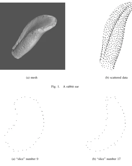
Example 4.1: As an application of this previous
interpo-lation method we were interested in a semi-implicit repre-sentation of a rabbit ear. The ear we took is illustrated by figure 1 where one can see a meshed and a scattered data representation. Late is obtained with 927 points. Cutting by horizontal planes, that is to say of equations z = c where c
is constant we formed 20 sets of 45 points, each set being include in a horizontal plane. Notice that we choose, at a first attempt to this problem, to take equally distributed planes. Now in every plane we have a “slice” of the rabbit’s ear (this is not really a slice since we have projected some points which were near this slice) which we have to interpolate. The slices number9 and 17 are showed in figure 2 below.
The next step in the previous algorithm is to approximate the 45 points in each “slice” by an algebraic curve implicitly represented. This is the more time-consuming step of the process. A way to perform it is to use a particular family of planar quartic curves called dinoid which are studied in [8] and that we are going to see in the sequel.
V. AN EXAMPLE OF SURFACE WITH SKELETON
We consider a special kind of semi-implicit surfaces which could be useful to provide simple models for compression or animation.
We choose a semi implicit surface represented by a family of planar curves whose real part is formed by a multiple point and an oval. In [8], we call such a curve a dinoid. The oval will modelize an active contour and the multiple point its skeleton following the general idea of Blum [9].
To illustrate this approach, we consider a family of quartic dinoid. First we give the equation f (x, y) = 0 of such a
curve when the singular point is at the origin.This imposes 3 conditions: the vanishing at the origin of f and of its two
partial derivatives, so f must be the sum of 3 homogeneous
polynomials of degree 2, 3 and 4. Setting y = sx, we get: g(x, s) = f (x, sx) = x2(f4(s)x2+ f3(s)x + f2(s)) = 0,
where fi are univariate polynomials of degree i. Then we
see that for each value of the slope s = y/x such that f4(s)f2(s) < 0, f (x, y), g(x, s) admits only two solutions
surrounding the origin. For instance for
f (x, y) = 16 x4+ x2y2+ y4+ 2 x3−2 xy2 +y3−10 x2−3 xy − 25 y2
we have
g(x, s) = (s4+ s2+ 16)x2−25s2+ (s3−2s2+ 2)x − 3s − 10.
In that case the curve defined byf is drawn in the following
picture. –4 –2 2 4 –1.5 –1 –0.5 0.5 1 1.5
We now consider a family of such curves, its semi-implicit equations are: L(x, y, z, t) = z − 5t + (1 + 2t)x − 1 40y, F (x, y, t) = 25 y2+ y4+ y3+ 16 x4−y2xt + 1/4 y2t2+ 2 x3 −31 4 t 3+ t4+ 1/8 t5−8 xt3+ 24 x2t2−32 x3t +63 2 xt 2 −33 x2t+y2x2−5/2 t2+10 xt−10 x2−xt4+3 x2t3−4 x3t2 +2 tx4+ y2t − 2 y2x + 3/2 yt − 3 yx.
Fort = 0 we recover the curve whose equation is f = 0.
The spanned surfaceS is drawn in the following picture.
In this case the skeleton of S is given by the parametric
equations:
x = t/2 y = 0 z = t2+11 2 t.
VI. USUAL DIFFERENTIAL GEOMETRIC INVARIANTS
Given a semi-implicitly represented surface, it is possible to compute at any regular point the usual differential geometric invariants such as :
• The equation of the tangent plane thus the normal, • The second fundamental form thus the curvatures.
Let us do it for a surface S passing by the origin and
represented by a family of plane curves parameterized by t
(the origin being obtained for t = 0). S is given by the
two equations: L(t, x, y, z) of degree one in x, y, z and of
possibly higher degree in t; F (t, x, y, z) of any degree in x, y, z, t. With our hypothesis they satisfy L(0, 0, 0, 0) = 0
, andF (0, 0, 0, 0) = 0.
The tangent space of S at the origin is generically the
projection of the tangent space at the surface defined by L
andF at (0, 0, 0, 0) in R4. So in order to compute the tangent
space we can truncate L and F and keep only their affine
Taylor expansions, that we callL1 andF1.
To be more specific let
L1:= lx + my + nz + pt, F1:= ax + by + cz + dt,
then the equation of the tangent space is:
T g := (−pa + dl)x + (−pb + dm)y + (dn − pc)z.
If p and d are both zero, then L1 and F1 should be
proportional in order that the origin is non singular on S,
in that case we keep either equation.
The 3 coefficients ofT g define the coordinates of the normal
atS at the origin.
The computation of the second fundamental form is more complicated. It amounts to compute an implicit equation ofS
near by the origin, truncated at orders greater than three. We take the Taylor expansions of L and F at order 3 in x, y, z
(a) mesh (b) scattered data
Fig. 1. A rabbit ear
(a) “slice” number 9 (b) “slice” number 17
Fig. 2. “Slices” of a rabbit ear
(we should not truncate also in t). Let us call them L2 and
F2. They are two polynomials inx, y, z, t.
We use a resultant to eliminatet between L2andF2and we
get a polynomial G(x, y, z) in x, y, z whose degree depends
on the degrees in t of L2andF2. Then we compute a Taylor
expansion at order 3 ofG at the origin and get a polynomial
of degree 2 which writes T g + Q1, withQ1 a quadratic form
inx, y, z. This provides a local equation of S at the origin.
Then it suffices to perform a change of coordinates (which preserves the metric), call X, Y, Z the new coordinates, so
that the previous local equation of S at the origin becomes Z + Q(X, Y, Z) = 0, where Q is a quadratic form. Finally
the second fundamental form for S at the origin is simply Q(X, Y, 0).
Example 6.1: Let
L = (1 + 2t)x − y + (1 + 5t)z + (−1 + 2t)t + t6x,
F = (−2 + t)x + (−3 + 4t)y + (−3 − 2t)z + (−4 + 2t)t
−2x2+ 5y2+ 2z2+ 3xy + 2xz + 5yz + t3x3.
Then the equation of the tangent plane at the origin is
6x − y + 7z = 0.
After formal computations described above we obtain the following local equation of S at the origin:
7z + 6x − y − 27yz + 12z2−23xy + 69x2+ 90xz + 3y2= 0.
We note that without the t6x term in the equation L the
local equation would have been different, namely:
6x − y + 7z + 3y2−27yz +46 3 xz −
37
3 xy + 12z
2+ 5x2.
This shows that the intermediate resultant computation was actually useful.
VII. SINGULARITIES AND SELF-INTERSECTION POINTS
An important problem in Computer Aided Geometric De-sign is the detection of singularities and self-intersection points of a 3D-surface. We describe a method to complete such a detection in case the considered surface is semi-implicitly represented.
LetS be a surface semi-implicitly represented by both
poly-nomials F (x, y, z, w; s, t) and G(x, y, z, w; s, t) of respective
bi-degree (k1, d1) and (k2, d2). A given point (x0 : y0 : z0 :
w0) of S ⊂ P3 is a self-intersection point if there exist two
distinct points(s1: t1) and (s2: t2) in P1 such that:
F (x0, y0, z0, w0; s1, t1) = G(x0, y0, z0, w0; s1, t1) = 0, and
F (x0, y0, z0, w0; s2, t2) = G(x0, y0, z0, w0; s2, t2) = 0.
By proposition 3.3 we know that an implicit equation of
S can be obtained as the determinant of the Sylvester matrix
of F and G with respect to the homogeneous variables s, t.
We denote by R(x, y, z, w) this Sylvester matrix and take
a given point p = (x0, y0, w0, z0) ∈ P3. If p is not on
S then clearly the kernel of R(p) is reduced to 0 since its
determinant is non-zero. Now if p is on S then obviously the
kernel of R(p)t (where t stands for transpose) is no reduced
to zero since it contains a multiple of the vector of monomials
(s0, t0)d1+d2−1, where (s0: t0) ∈ P1 is such that
F (x0, y0, z0, w0; s0, t0) = G(x0, y0, z0, w0; s0, t0) = 0
(observe that we can consequently compute (s0 : t0)). If
now p is a self-intersection point of S then the dimension
of the kernel of R(p)t is at least 2 since this kernel contains
both non collinear vector of monomials (s1, t1)d1+d2−1 and
(s2, t2)d1+d2−1. Thus a necessary condition for a point p to
be a self-intersection point is thatrank(R(p)) ≤ d1+ d2−3.
Similarly, if(p; s0, t0) is a singular point of the semi-implicit
representation such that
F (p; s0, t0) = G(p; s0, t0) = 0 and
∂sF (p; s0, t0) = ∂sG(p; s0, t0) = 0,
then both non-collinear monomial vectors(s0, t0)d1+d2−1and
∂s((s0, t0)d1+d2−1) and in the kernel of R(p). In other words,
singularities and self-intersection points of the semi-implicit representation of S are located on the zero locus of the (d1+ d2−2) × (d1+ d2−2) minors of the Sylvester matrix
R(x, y, z, w) in P3.
VIII. INTERSECTING A SEMI-IMPLICIT SURFACE
In this section we investigate the intersection problems between different curves and surfaces. Our aim is to show that semi-implicit representations are well adapted to these operations; being an intermediate representation between pa-rameterized and implicit representations, they gather their advantages. We illustrate it on the three main configurations, say the intersection between a semi-implicit surface and a parameterized curve, a parameterized surface a semi-implicit surface.
HereafterS denote a surface semi-implicitly represented by
both polynomials F (x, y, z, w; s, t) and G(x, y, z, w; s, t) of
respective bi-degree (k1, d1) and (k2, d2). A. With a parameterized space curve
Let g0, g1, g2, g3, be four homogeneous polynomials in
both variables s, t of the same degree d, and let C be the
parameterized curve (we write here, for simplicity, the affine version of this parameterization, i.e. sett = 1 and w = 1)
C : µ x = g1(s) g0(s) , y = g2(s) g0(s) , z = g3(s) g0(s) ¶ .
We assume w.l.o.g. that there is no base point, i.e. that
gcd(g0, g1, g2, g3) is a constant. Our goal is to compute the
intersection ofC and S. First by proposition 3.3 we know that
there exists a resultant matrixR(x, y, z) whose determinant is
an implicit representation ofS. Now substituting respectively x, y, z by g1(s) g0(s), g2(s) g0(s) and g3(s) g0(s) we obtain a matrix R(s)
depending on the alone variable s that we can decompose
as
R(s) = Rdsd+ · · · + R0,
where the coefficientsRi are numerical matrices of the same
size than R(s). Now we are looking for the values of s such
that this surface and the curve intersect at C(s), that is such
that the determinant ofR(s) vanishes. This is relate to known
methods to solve such “equation” [10], [11]. We have to compute the vectors v (indexed by monomials ins) such that R(s)tv= 0. The intersection problem can thus be transformed
into the following generalized eigenvector problem (solved by efficient and stable numerical algorithms):
0 I . .. . .. 0 I −Rt 0 . . . −R t d−1 − I . .. I Rt d w= 0,
where I is the identity matrix and w denote the vector
(v, sv, · · · , sd−1v)t.
Such a tool can be useful in ray tracing techniques which involve the intersection of a surface with a line, and similarly to inside/outside positioning of a point with respect to a semi-implicit surface.
B. With a parameterized surface
Letf0, f1, f2, f3 be four homogeneous polynomials of the
same degree d in the homogeneous variables t0, t1, t2. They
define a parameterized surface in P3 (here again we present the affine point of view, settingt0= 1 and w = 1):
S′: µ x = f1(t1, t2) f0(t1, t2) , y = f2(t1, t2) f0(t1, t2) , z = f3(t1, t2) f0(t1, t2) ¶ .
Our goal is here again to represent the intersection curve C of
S and S′. We assume for simplicity that the parameterization
of S′ is without base point (i.e. f − 0, f
1, f2, f3 have no
Bezout’s theorem we deduce that C is of degree d2(k 1d2+
k2d1).
By proposition 3.3 we know that there exists a resultant ma-trixR(x, y, z) whose determinant is an implicit representation
ofS. Substituting respectively x, y, z by f1(t1,t2)
f0(t1,t2),
f2(t1,t2)
f0(t1,t2)and
f3(t1,t2)
f0(t1,t2) we obtain a matrixR(t1, t2) depending only on both
variablest1 andt2. Its determinant define a curve (implicitly
represented) which is of degree d(k1d2+ k2d1), that is to
say of lower degree than C. This curve is a representation of the intersection curve C since every point t1, t2 such that
R(t1, t2) = 0 can be sent on C by the parameterization of S′.
This method consisting of representing an intersection space curve by a birational plane curve is very useful in practice. It has been widely studied in the works of D. Manocha [10], [11] in the context of the intersection of two parameterized surfaces. We thus show here that we can also represent in this process one of the surface semi-implicitly instead of parametrically.
C. With a semi-implicit surface
In the case of the intersection of two semi-implicit surface we can, as in the previous paragraph, obtain a plane curve which is birational to the intersection curve. To be more precise let S′ be a semi-implicit surface defined by both
polynomials F′(x, y, z, w; s′, t′) and G′(x, y, z, w; s′, t′) of
respective bi-degree (k′
1, d′1) and (k′2, d′2). We are interesting
in the intersection (space) curve of S and S′ in P3 (with
homogeneous variablesx, y, z, w).
As previously we are going to use a resultant. However we need a more general resultant that the Sylvester one. We are going to use the resultant of four homogeneous polynomials in four homogeneous variables. This resultant was introduced by Macaulay [12] and has been since widely studied [13]–[15] being very useful in a wide range of applications (see e.g. [15] for applications in Computer Aided Geometric Design). For a nice introduction to this topic we refer the reader to [2].
It appears that the resultants ofF, G, F′andG′with respect
to the homogeneous variables x, y, z, w is a polynomial in s
and s′. It vanishes at a given points
0, s′0 if and only if both
surfaces S and S′ intersect with these parameters, i.e. there
exists (at least) a point x ∈ P3 such that
F (x; s0) = G(x; s0) = F′(x; s′0) = G′(x; s′0).
Let us denote by R(s, s′) this polynomial. It defines a plane
curve in the plane of coordinates(s, s′) which is in
correspon-dence with the intersection (space) curve ofS and S′. We can
therefore, as in the previous paragraph, apply all the techniques developed by many authors on such a representation of the intersection curve.
IX. CONCLUSION
In this paper we explained how one can develop new algebraic models for representing shapes together with effi-cient algorithms to compute their local differential geometric invariants, their singularity locus and their intersections. We illustrated our approach with simple examples. To represent
a complex shape in our context we will decompose it into smaller parts. Each of these parts should be sliced in order to get a family of curves having similar shapes. Therefore there are at least two main next tasks : one is a detection/recovery problem, and the other one is to reconstruct a model from a set of such parts. In a future work we will compare our algebraic approach which is rigid by nature (this allows to handle complex shapes with few parameters) with other more flexible techniques.
REFERENCES
[1] L. Bus´e and A. Galligo, “Semi-implicit representations of surfaces inP3
, resultants and applications,” to appear in J. of Symbolic Computation. [2] D. Cox, J. Little, and D. O’Shea, Using algebraic geometry, ser.
Graduate Texts in Mathematics. Springer, 1998.
[3] D. Hansford and G. Farin, “Curve and surface constructions,” in
Hand-book of computer aided geometric design. Amsterdam: North-Holland,
2002, pp. 165–192.
[4] M. Gasca and T. Sauer, “On the history of multivariate polynomial interpolation,” J. Comput. Appl. Math., vol. 122, no. 1-2, pp. 23–35, 2000, numerical analysis 2000, Vol. II: Interpolation and extrapolation. [5] V. Pratt, “Direct least-squares fitting of algebraic surfaces,” Comput.
Graphics, vol. 21, no. 4, pp. 145–152, 1987, SIGGRAPH ’87 (Anaheim,
CA, 1987).
[6] C. L. Bajaj and I. Ihm, “Algebraic surface design with hermite inter-polation,” ACM Transactions on Graphics, vol. 11, no. 1, pp. 61–91, 1992.
[7] T. Dokken, “Approximate implicitization,” in Mathematical methods for
curves and surfaces (Oslo, 2000), ser. Innov. Appl. Math. Nashville, TN: Vanderbilt Univ. Press, 2001, pp. 81–102.
[8] A. Galligo and P. Hermunn, “Study of a family of planar quartic curves,” in preparation.
[9] H. Blum, “A transformation for extracting new descriptors of shapes,” in
Models for the Perception of Speech and Visual Form, ser. Cambridge,
vol. MIT Press, 1967, pp. 362–380.
[10] J. F. Canny and D. Manocha, “A new approach for surface intersection,”
International Journal of Computational Geometry and Applications,
vol. 1, no. 4, pp. 491–516, 1991.
[11] S. Krishnan and D. Manocha, “An efficient surface intersection algo-rithm based on lower dimensional formulation,” ACM Transactions on
Computer Graphics, vol. 16, no. 1, pp. 74–106, 1997.
[12] F. Macaulay, “Some formulae in elimination,” Proc. London Math. Soc., vol. 33, pp. 3–27, 1902.
[13] J.-P. Jouanolou, “Le formalisme du r´esultant,” Adv. in Math., vol. 90, no. 2, pp. 117–263, 1991.
[14] I. Gelfand, M. Kapranov, and A. Zelevinsky, Discriminants, Resultants
and Multidimensional Determinants. Birkh¨auser, Boston-Basel-Berlin, 1994.
[15] L. Bus´e, M. Elkadi, and B. Mourrain, “Using projection operators in computer aided geometric design,” in Topics in Algebraic Geometry and
Geometric Modeling, ser. Contemporary Mathematics, vol. 334. AMS,