Agulhas ring injection into the South Atlantic during glacials and interglacials

(1)

HAL Id: hal-00298491

https://hal.archives-ouvertes.fr/hal-00298491

Submitted on 17 Mar 2008

HAL is a multi-disciplinary open access

archive for the deposit and dissemination of sci-entific research documents, whether they are pub-lished or not. The documents may come from teaching and research institutions in France or abroad, or from public or private research centers.

L’archive ouverte pluridisciplinaire HAL, est destinée au dépôt et à la diffusion de documents scientifiques de niveau recherche, publiés ou non, émanant des établissements d’enseignement et de recherche français ou étrangers, des laboratoires publics ou privés.

Agulhas ring injection into the South Atlantic during

glacials and interglacials

V. Zharkov, D. Nof

To cite this version:

V. Zharkov, D. Nof. Agulhas ring injection into the South Atlantic during glacials and interglacials. Ocean Science Discussions, European Geosciences Union, 2008, 5 (1), pp.39-75. �hal-00298491�

(2)

OSD

5, 39–75, 2008

Agulhas ring injection into the

South Atlantic V. Zharkov and D. Nof

Title Page Abstract Introduction Conclusions References Tables Figures ◭ ◮ ◭ ◮ Back Close Full Screen / Esc

Printer-friendly Version Interactive Discussion Ocean Sci. Discuss., 5, 39–75, 2008

www.ocean-sci-discuss.net/5/39/2008/ © Author(s) 2008. This work is licensed under a Creative Commons License.

Ocean Science Discussions

Papers published in Ocean Science Discussions are under open-access review for the journal Ocean Science

Agulhas ring injection into the South

Atlantic during glacials and interglacials

V. Zharkov1and D. Nof1,2

1

Geophysical Fluid Dynamics institute, Florida State University, FL, USA

2

Department of Oceanography, Florida State University, FL, USA

Received: 22 November 2007 – Accepted: 3 December 2007 – Published: 17 March 2008 Correspondence to: D. Nof (nof@ocean.fsu.edu)

(3)

OSD

5, 39–75, 2008

Printer-friendly Version Interactive Discussion

EGU Abstract

Recent proxies analysis suggest that, at the end of the last glacial, there was a signifi-cant increase in the injection of Agulhas rings into the South Atlantic (SA). This brought about a dramatic increase in the salt-influx (from the Indian Ocean) into the SA helping re-start the then-collapsed meridional overturning cell (MOC), leading to the

termina-5

tion of the Younger Dryas (YD). Here, we propose a mechanism through which large variations in ring production take place. Using nonlinear analytical solutions for eddy shedding we show that there are restricted possibilities for ring detachment when the coast is oriented in the north-south direction. We define a critical coastline angle below which there is rings shedding and above which there is almost no shedding. In the

10

case of the Agulhas region, the particular shape of the African continent implies that rings can be produced only when the retroflection occurs beyond a specific latitude where the angle is critical. During glaciation, the wind stress curl (WSC) vanished at a latitude lower than that of the critical angle, which prohibited the retroflection from producing rings. When the latitude at which the WSC vanishes migrated poleward

to-15

wards its present day position, the corresponding coastline angle decreased below the critical angle and allowed for a vigorous production of rings. Simple process-oriented numerical simulations (using the Bleck and Boudra model) are in very good agreement with our results and enable us to affirm that, during the glacials, the behavior of the Agulhas Current (AC) was similar to that of the modern East Australian Current (EAC),

20

for which the coastline slant is supercritical.

1 Introduction

In a recent article (Zharkov and Nof, 2007, ZN, hereafter) we examined the develop-ment of a nonlinear retroflection eddy and constructed a solution describing the time-evolution of the ring and the mass flux going into it. Here, we shall consider the later

25

stages in the eddies evolution – their detachment and propagation away from their gen-40

(4)

OSD

5, 39–75, 2008

Printer-friendly Version Interactive Discussion eration area. We will focus on the angle of the coastline slant, supposing the incoming

current to be parallel to it, and show that, when this angle exceeds a critical value, the frequency of eddy detachment is severely restricted. We shall see that this may explain why very few Agulhas eddies were injected into the Atlantic during the Last Glaciation Maximum (LGM) and the Younger Dryas (YD),

5

1.1 Observational background

The Agulhas Current (AC) rings transport water from the Indian Ocean to the South Atlantic (SA) and, therefore, contribute to the near-surface return flow of the North At-lantic Deep Water (NADW) from the Pacific and Indian Oceans to the North AtAt-lantic. The rings common transport represents a significant part of the meridional overturning

10

circulation (MOC) (Gordon et al., 1987; Wejer et al., 1999; van Veldhoven, 2005; Lut-jeharms, 2006) but their most important component comes from their anomalous salt content which brings in a salt anomaly five times as large as that of the Mediterranean outflow. The shedding of Agulhas rings is not a regular event. Some rings immediately split after formation, while others are recaptured by the retroflection. Furthermore,

al-15

though the typical frequency of shedding is 4–5 times a year (Schouten et al., 2002), intervals of over half-a-year without a ring-shedding event have been observed (Goni et al., 1997; van Veldhoven, 2005).

The recent paleoceanographic proxies analysis of Rau et al. (2002) and Peeters et al. (2004), suggest that the Indian-Atlantic water exchange varied greatly throughout

20

the past 550 000 yr, having been enhanced during interglacials and strongly reduced during glacial intervals. One can tentatively suggest on the basis of Howard and Prell (1992), and Berger and Wefer (1996), that the glacial Agulhas leakage was completely shut-off due to a northward migration of the wind bands. Strictly speaking, however, this explanation is incorrect as the wind field controls the ocean interior but not the AC,

25

i.e., rings can still propagate along the coast and penetrate into the Atlantic even when the wind stress curl vanishes north of the continental southern termination.

(5)

OSD

5, 39–75, 2008

EGU

glacial Atlantic MOC could easily collapse. With a smaller input from Agulhas rings, the salt content of the Atlantic reduced and decreased the strength of the MOC. Because an increase in ring activity brings more salt to the Atlantic Ocean (Knorr and Lohmann, 2003), Peeters et al. (2004) suggestion that there was vigorous Agulhas ring activity at the end of each glacial might explain how a collapsed MOC restarted. The onset

5

of increasing Agulhas leakage during late glacial conditions took place when glacial ice volume was maximal, which suggests the crucial role of Agulhas leakage in glacial terminations, timing of inter-hemispheric climate change, and the resulting resumption of the Atlantic MOC. The question that we address here is: Why were there more rings during the end of the glacial?

10

1.2 Salt balance

The importance of the Agulhas rings salt-flux to the MOC was already established by Weijer et al. (2001) and Speich et al. (2006) but it is useful to re-capture here the main aspects of the issue. The annualized volume transport associated with an average Ag-ulhas ring is estimated to be between 0.5 and 1.5 Sv. It is not a trivial matter to estimate

15

the salt anomaly introduced by the rings. Many conventional calculations take the salt difference between each ring and its immediate environment in the Southeastern At-lantic and calculate the contributed anomaly on this basis. This grossly underestimates the true contributed anomaly because the volume flux of the rings (Q_R which is, say, 10 Sv) is so large that the whole southeastern Atlantic is full of relatively salty water

20

from old rings.

To correctly do the estimate, one needs to consider the salinity that the SA would have had in the absence of the rings. If one takes the SA salinity (S) in the absence

of Agulhas rings to be slightly higher than the AAIW salinity (say, 34.5 PSU) and the rings salinity to be one PSU higher, 35.5 PSU, then one finds that the salinity anomaly

25

(Q_R∆_{S) contributed by the rings is roughly 10 SvPSU. This is about five times the} buoyancy anomaly contributed by the Mediterranean Sea or the Bering Strait.

Taking the MOC transport to be, say, 15 Sv, and applying a simple interpolation, we 42

(6)

OSD

5, 39–75, 2008

Printer-friendly Version Interactive Discussion find that a hypothetical removal of the entire Agulhas rings influx today (10 Sv of water

1 PSU saltier) would lower the MOC salinity by 0.7 PSU. This is about half of what would be sufficient to collapse the MOC altogether under present day conditions [see Nof and Van Gorder, 2003, (their) Fig. 2] so a simple linearization suggests that the MOC transport will be reduced by 50%.

5

1.3 The glacial-interglacial hypothesis

With basic Sverdrup dynamics, the meridional velocity within the ocean interior is pro-portional to the wind stress curl (WSC), whereas the zonal velocity is propro-portional to both the meridional gradient of the WSC and the distance from the eastern boundary of the basin. This linear Sverdrup flow occupies most of the basin, and, when the

10

basin is closed, its net meridional transport is compensated for by a WBC flowing in the opposite direction. The meridional component of the Sverdrup transport vanishes at the latitudes where the WSC vanishes (∂τ_x/∂y=0). This implies that the flow at

these latitudes is purely zonal, so that, for a closed basin, the vanishing of the WSC also defines the location of the WBC separation.

15

However, most ocean basins are not closed. The Indian Ocean is wide open so sig-nificant WBC-induced meridional leakages can occur across the latitude of vanishing WSC. Having said that, we should also note that, since the vanishing curl is approxi-mately the same all around the globe, northward leakages must be compensated for by southward flow within boundary currents. Also, note that the position of zero WSC

20

in this region is roughly at the Subtropical Convergence Zone about 45◦S (de Ruijter, 1982), which is beyond the termination of the continent. In view of these, we shall take the position of vanishing WSC to be the retroflection latitude but keep in mind that there can be leakages across it near the boundary. Furthermore, we will assume that the shift in the position of retroflection roughly follows the shift in the WSC (Fig. 1).

25

The above is easier said than done, because it is difficult to determine the exact lat-itude of the zero WSC in the Western Indian Ocean during the LGM and the YD. On one hand, it could be inferred from Peeters et al. (2004) that the Subtropical

(7)

Conver-OSD

5, 39–75, 2008

EGU

gence Zone was 2–5◦ farther north during the YD. On the other hand, Gasse (2000) and Esper et al. (2004) argue that the shift of the westerly wind belt was much larger, as much as 25◦. This is supported by the analysis of proxies from the Pacific, where the shifting process was studied via the position of the (somewhat weaker) East Aus-tralian Current (EAC). Note that, although the EAC is weaker than the AC, it is the

5

Pacific analog of the AC. According to Martinez (1994), Kawagata (2001), Martinez et al. (2002), and Bostock et al. (2006), there was a large northward shift of the Tasman Front (a branch of the EAC) from its present latitude of 33◦S to about 25◦S during the last glacial. Tilburg et al. (2001) suggested that the WSC is not exactly zero at the lati-tude of the EAC separation, implying that the EAC does not separate completely from

10

the coast. However, the WSC is minimal, and its gradient is maximal at the latitude of the formation of the Tasman Front, implying that the glacial/interglacial shifts of the EAC separation occurred mainly due to the shifts of the WSC.

In view of these aspects, we shall suppose that the Agulhas retroflection latitude, during both the LGM and the YD, was between 25◦S and 31◦S (instead of its present

15

position of about 38◦S). We shall show that, with such a shift, the coastline slant in the neighborhood of the retroflection during the glacials was between 50◦ and 70◦, which severely restricted the formation of eddies. This is because the rings’ long-wall drift speed was small so that they were not removed quickly enough from their formation region to avoid being recaptured. We shall see that this slower long-wall migration rate

20

(in case of nearly meridional coastline) is due to the obvious blocking imposed by the wall.

We note here in passing that the slant of the Australian coastline at the point of the present day EAC separation is about 65◦, roughly the same as that of the glacial AC. This explains why EAC rings are not usually found around the southern tip of

25

Tasmania – the coastline slant is just too high to allow rings shedding. As in the Agulhas case, anticyclonic eddies are detached from the EAC by the pinching-off of poleward meanders. However, in contrast to the present day Agulhas case, the eddies often coalesce with the EAC again (Nilsson et al., 1977; Andrews and Scully-Power, 1976;

(8)

OSD

5, 39–75, 2008

Printer-friendly Version Interactive Discussion Nilsson and Cresswell, 1981; Sokolov and Rintoul, 2000).

The important aspect here is that none of the EAC rings (which, without the slanting coastline idea, would be the analogs of present day Agulhas rings in the Southeastern Atlantic) is found west of Tasmania.

1.4 Present approach

5

We shall begin our study by examining the condition of ring shedding due toβ (Sect. 2).

We will look at the theoretical ranges of detached eddies radii, their propagation speeds, and their periods of detachment, as well as the average amount of mass flux going into the rings. To examine our glacial-interglacial hypothesis regarding the critical slant angle, we shall analyze the dependence of the above-mentioned aspects on the

10

slant angle and other model parameters. We will also present the results obtained from numerical simulations (using a “reduced gravity” model of the Black and Boudra type), which visually elucidate two different regimes of eddy generation.

The paper is organized as follows. Section 2 is devoted to the definition of lower and upper boundaries of the ring dimensions, position and drift speed. In Sect. 3, we

15

analyze the results of our analytical modeling, and examine the critical angles of the slant. In Sect. 4, we give the results of our numerical simulations for sub-critical and supercritical slant angles, and compare them with our analytical calculations. Finally, in Sect. 5, we summarize the results and give the conclusions regarding the glacial-interglacial hypothesis.

20

2 Shedding

2.1 Governing equations and the long-wall eddy propagation rate

We begin with the nonlinear momentum-flux and mass conservation equations for the retroflection eddy [also referred to as the “basic eddy” (BE)] growth as given in ZN. The

(9)

OSD

5, 39–75, 2008

EGU

most relevant combinations of the above are (their) Eqs. (3.21) and (3.23), which are very useful but cumbersome and, therefore, are not reproduced here. All the following formulae and computations are based on solutions of these equations for,

R=R(t), Φ=Φ(t), H=H(t). (1)

Here,R is the radius of developing eddy, Φ the ratio of the mass-flux going to the BE

5

and the total incoming mass-fluxQ, and H is the thickness of the upper (moving) layer

outside the retroflection area. All depend onQ (incoming mass flux), h0(thickness of the upstream upper layer along the coast),g′(reduced gravity),f (Coriolis parameter), α (twice Rossby number), β (meridional gradient of f ) and γ (slant of the coast). We

again use the tilted coordinate system (ξ, η) adopted by ZN. (For convenience, all

10

variables are defined both in the text and the Appendix.)

Following Nof (2005), we consider ring shedding due toβ which, in the open ocean,

forces the eddies westward (Nof, 1983) according to,

Cx≈−( αβR2

12 )

α(2−α)f2R2+24g′H

α(2−α)f2_R2₊₁₆_g′_H. (2)

We then suppose that, in the case of a non-zonal wall, this velocity component along

15

the wall is simply reduced due to the geometrical blocking of the wall,

C_ξ=_C_x_cos_γ. ₍₃₎

The above is not a rigorous derivation of the long-wall drift speed but it will later be con-firmed with our numerical simulations. We also note that this assumption is supported by the numerical calculations of Arruda et al. (2004), which demonstrated that no eddy

20

detachment occurs in the case of a meridional wall (γ=90◦

). The so-called image-effect is neglected here on the ground that there is no image-effect in the limitH → 0(Shi and

Nof, 1994) andH is not very large (relative to the maximum eddy thickness) in most

of our analysis. Our numerical simulation will later support this assumption even forH

that is not small, probably because the rings are formed off the wall.

25

(10)

OSD

5, 39–75, 2008

Printer-friendly Version Interactive Discussion 2.2 Lower and upper boundaries for the radii of eddies and periods of their

detach-ment

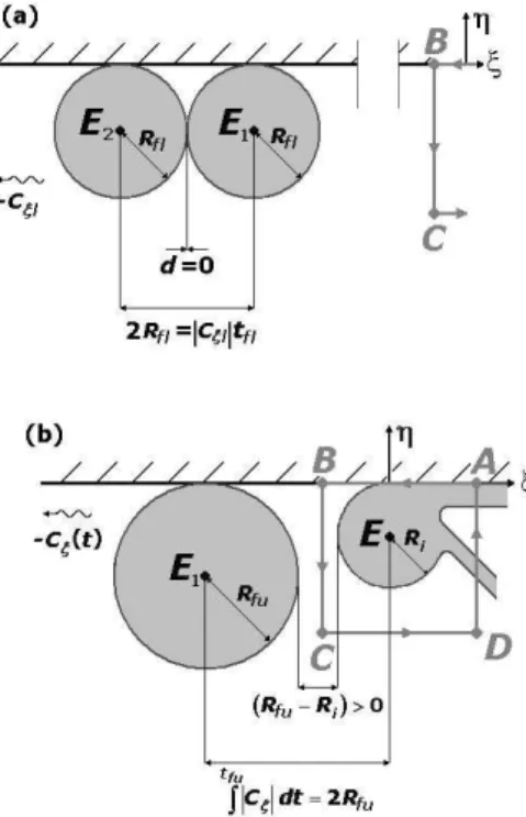
On the basis of the downstream structure (Fig. 2a), the generation period for each individual eddy is taken as,

t_f= (2R_f+_{d ) /}C_{ξ f}

, (4)

5

whered is the distance between two consecutive eddies, and the subscript f denotes

the final value. The “lower boundary” for the final eddy size (Rf l) can be obtained using

the “kissing condition” (i.e.d =0, Fig. 2a). In that case, (2), (3) and (4) give,

t_{f l}= 24 αβR_{f l}cosγ α(2 − α)f2R_{f l}2+16g′Hf l α(2−α)f2_R2 f l+24g ′_H f l . (5)

Equation (5) implies thatRf l=R (tf l) and Hf l=H (tf l) and will be solved numerically.

10

Next, we derive the intricate “upper boundary” (R_{f u}) for the final BE size (i.e., the detachment size). For this purpose, consider the configuration shown in Fig. 2b. Dur-ing the generation period, the eddy is movDur-ing along the axis ξ with the velocity Cξ,

which is a function of time and is defined by (2)–(3). The displacement of the BE from its initial position during the generation period is

t_f R 0 C_ξ

d t. We note that, when this

15

displacement equals the final diameter of the eddy (i.e., 2Rf), then it must be detached

because, at this point in time, it osculates the already generated eddy downstream (whose radius must also beR_f).

Since the distance between the centers of the two consecutive eddies may exceed the sum of their radii, we can place the segment of the integration contour surrounding

20

the area of the BE between the two eddies (Fig. 2b), indicating that the formation of the second eddy is now in progress as the first one has already been fully developed

(11)

OSD

5, 39–75, 2008

EGU

and shed. In view of this, we write the condition of “upper boundary” in the form,

t_{f u} Z 0 C_ξ d t=2R_{f u}, (6)

which is an (integral-algebraic) equation forR_{f u}.

Physically, the “upper boundary” corresponds more directly to the detachment of eddies, whereas the “lower boundary” corresponds to a condition for the formation

5

of an eddy chain. Consequently, the eddies can detach and propagate out of the retroflection area if the condition,

R_{f l}≤R_{f u} (7)

is satisfied. This condition is certainly valid for the “imbalance paradox” (Nof, 2005), for which it is easy to show that whenRf l significantly exceeds Ri (the initial radius,

10

see ZN), then R_{f u}=21/5R_{f l}. For the upper boundary case (R_f=_R

f u), one obtains d =d_u=2R_{f u}, implying that the distance between two consecutive eddies centers can-not exceed the eddy diameter.

3 Analysis

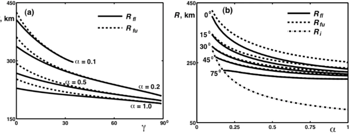
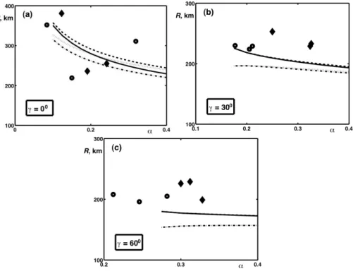
3.1 The “lower” and “upper” boundaries and the critical angle

15

We (numerically) solved the corresponding nonlinear differential equations reflecting the momentum-flux and mass conservation [given as (3.21) and (3.23) in ZN], sub-ject to conditions (1–7). For this purpose, we used: Q=70 Sv, g′

=2×10−3m s−2 and

f =8.8×10−5s−1(corresponding to 35◦of latitude). We took zero and 300 m forh0, and 2.3×10−11 and 6×10−11m−1s−1 forβ. Alpha (α) and γ varied between 0.1 and 1.0,

20

and between zero degrees and 89◦, respectively. The results, all of which satisfy our two limiting boundaries, are shown in Fig. 3, which displays the graphs ofRf l and Rf u

(12)

OSD

5, 39–75, 2008

Printer-friendly Version Interactive Discussion as functions ofγ. We see that, for each α, the radii decrease with growing γ ,

gradu-ally approaching each other, and fingradu-ally converging. This convergence occurs whenγ

exceeds 70◦ forα>0.4, and 60◦

forα≈0.2. When α is quite small (0.1 in the figure),

the curves converge very quickly and then break off. That occurs because, in this case whenγ is not very small, the β-force overwhelms the forces of the currents already at

5

the initial moment (whenR=R_i) so the BE is forced into the wall instead of growing. For these conditions,R_{f l}, andR_{f u}cannot be defined in terms of our model. To clarify this effect further, we plottedRi,Rf l, andRf u versusα (starting from α=0.1) for different

values ofγ (Fig. 3b). We see that the curves of R_{f l} andR_{f u} forγ≥45◦

start from the curveR_i, that is, they are defined forα=0.1 only when γ≤30◦

, and they are nearly

con-10

vergent. This convergence extends further with increasingα as the corresponding γ

grows. In addition, although bothR_{f l} andR_{f u}decrease withα, for γ≈75◦

this decrease becomes insignificant.

Figure 4 shows the periods of detachmenttf l andtf u(left panel) and the velocitiesCξl

andC_ξuof detached eddies whose radii areR_{f l} andR_{f u}(right panel). It is seen that the

15

detachment period decreases with growingα; however, it increases with increasing γ,

tending to infinity for the case of a nearly meridional wall (γ→90◦). This was obviously expected because in this caseCξ→0. Indeed, the curves ofCξconverge monotonically

to zero for each value ofα except 0.1. Convergence of curves corresponding to lower

and upper boundaries is seen here, too. Figures 3 and 4 suggest that eddy detachment

20

becomes restricted whenγ is sufficiently large, as well as when it is not large but α is

sufficiently small.

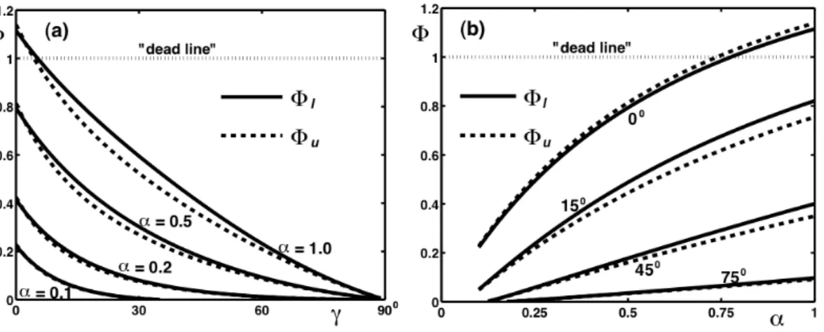
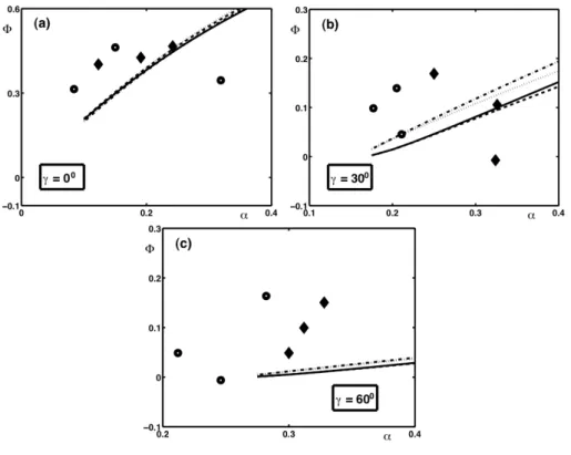
3.2 The mass flux going into the eddies

We will now estimate the ratio of the mass flux that goes into the rings and the incoming flux upstream (Φ). Because Φ depends on time, it can be obtained by averaging

25

(13)

OSD

5, 39–75, 2008

EGU

with two different values:

Φ_l=_t−1 f l t_{f l} Z 0 Φ_{d t, Φ}_u=_t−1 f u t_{f u} Z 0 Φ_{d t,}

meaning that Φ is averaged over the period of detachment.

Since Φ grows monotonically with time only whenγ=0◦and decreases for all other angles, we expect the (averaged) value for γ=0◦

to be greater for longer period of

5

formation, namely, Φ_u>Φl. Otherwise, when the wall is non-zonal, greater averaged

values are expected for shorter periods, namely, Φu<Φl. This is clearly demonstrated

in Fig. 5 showing plots of Φ versusγ for different α (left panel), and as functions of α for different γ (right panel). Here, we plotted the “deadline” in analogy with that of

Fig. 5 in ZN, meaning that the “vorticity paradox” occurs in the area above this line. As

10

expected, averaged values of Φ increase withα and decrease with γ. If the parameter

are such that the curves ofR_{f l} and R_{f u} converge, then the curves of Φ_u and Φ_l also converge (though this convergence is weaker).

The curves of Φ_u and Φ_l in Fig. 5a decrease monotonically to zero, and, when considered separately for fixedα, they intersect each other at the point corresponding

15

to γ between 1.5◦ and 2.5◦. The starting values are above the deadline for α≥0.8;

nevertheless, even the maximal values, corresponding toα=1, are considerably less

than 4/3, because the instant values of Φ are much less than unity at the beginning of the eddy development. Forγ≥6◦, all the curves are below the deadline. Note that, in the case ofα=0.1, the curves in Fig. 5a reach zero when the corresponding curves of

20

R_{f l} andR_{f u} in Fig. 3a are terminated. In Fig. 5b, Φ increases with γ. For γ=0◦ (zonal wall), the corresponding waves cross the deadline forα≈0.75, and when γ≥15◦, the corresponding waves are below the deadline everywhere. The rate of increase in Φ gradually diminishes with increasingγ. We note here that we obtained experimental

values of Φ≈0.15 every time γ exceeds 60◦, suggesting the existence of a critical angle

25

above which almost no eddies are detached. 50

(14)

OSD

5, 39–75, 2008

Printer-friendly Version Interactive Discussion 3.3 Varyingh0andβ

As mentioned, the influence of increasingh0is not significant. When we useh0=300 m instead of zero, the decrease in R_{f l} and R_{f u} with γ becomes more significant. In

the case α>0.1, the corresponding curves start from almost the same values as in

Fig. 3a, for γ=0◦

, but tend to the range between 170 and 180 km, when γ→90◦ . In

5

this connection, their converging curves ofR_{f l} andR_{f u}forα=0.2 intersect the ones for α=0.4, exhibiting smaller limiting (for γ→90◦) values. The values ofRf l andRf uat the

point of termination forα=0.1 are nearly 245 km instead of 295 km for h0=0.

The curves of R_{f l} and R_{f u} versus α become more spread out than in Fig. 3b,

es-pecially for γ≥45◦ and near the curve of Ri, where they even rise slightly and reach

10

maximal values, (240, 212, and 193 km forγ = 45◦, 60◦, and 75◦, respectively). Note thatR_i also decreases with increasingh0. The effect of increasingh0 on the period of eddy generation is less significant. The increase intf l andtf uwith increasingγ occurs

only slightly faster. Finally, the influence ofh0on the averaged values of Φ, as well as on the velocities of detached eddies, is very weak.

15

As expected, changing the parameter β leads to quantitative changes. When we

use the magnified value ofβ (i.e., 6×10−11m−1s−1), we find that the final eddy radius is reduced by about 20%. The boundary values of the detachment period are reduced approximately twice. The reduction in Φ does not exceed 10%, and the velocities of the detached eddies increase by about 60%. Since the initial eddy radius does not depend

20

on β, the decrease in final radii implies that there is a range of α and γ for which

the BE cannot grow at all. For example, when α=0.1, the considered parameters of

the detached eddies could be defined only in the case of a zonal wall (γ=0◦). When

γ=75◦

, they could be defined only whenα>0.3 (instead of α>0.17 for the natural value

ofβ). Therefore, the curves terminate when α is less then 0.3, instead of the natural β

25

termination occurring whenα=0.1 (Fig. 3a).

Despite the reduction, the final radii are still greater than the typical observational values (see ZN, Sect. 1). For example, whenγ=15◦

(15)

OSD

5, 39–75, 2008

EGU

both approximately 275 km, but they change to 170 and 180 km, respectively, when

α increases to unity. At the same time, tf l and tf u change from 135 to 20 and 25 d,

respectively. Therefore, if the potential vorticity (PV, related toα, see ZN) of the eddies

is nearly zero, the magnified value ofβ gives noticeably reduced values for the

detach-ment period, which naturally is 60–90 d (Byrne et al., 1995; Schouten et al., 2000). If

5

α is about 0.2–0.3, the agreement is better.

4 Numerical model simulations

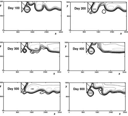
4.1 The numerical model

We used the Bleck and Boudra (1986) reduced gravity isopycnic model, the description of which was already presented in ZN and need not be repeated here. We comment

10

here only on the simulation of the detached eddies. We initialized the retroflection from a point along the wall that was about 300 km north of the termination of the continent. However, we also conducted some experiments starting with a current retroflecting shortly after its entrance into the basin. In that case, we observed that the current behaved similarly to the case where the incoming flow was zonal (though it did so after

15

a longer period of development). We did not obtain any plots of developing retroflection from a non-zonal wall. Our modeled time was long (about 210 d) so even when the eddies’ PV was initially small, it was ultimately altered significantly by the cumulative effects of friction during the experiment. Therefore, in our quantitative comparisons, we always obtained data for nonzero PV and averaged the values ofα over time.

20

4.2 Varying the slant

To accelerate the detachment of the rings and make our runs more economical we chose the magnified value ofβ for most of our experiments. In the experiments with a

naturalβ, the period of detachment usually exceeded 200 d but qualitative differences

(16)

OSD

5, 39–75, 2008

Printer-friendly Version Interactive Discussion in the evolution of the BE, caused by changingβ, were not noted. Of course, we could

not perform numerical simulations in which Φ would exceed unity.

(i) Zonal coastline: As mentioned, in the case of zonal incoming current, we were obliged to take a relatively high value for the viscosity coefficient. Although we fixed the parameters so that we can plot the thicknesses every ten days, the starting value

5

ofα=1 had already approached 0.4 by the time of fixing the parameters for the first

plot. At that point, we identified a chain of four eddies that had already partially formed and begun to move along the wall. The first eddy was separated, and the next three were almost kissing each other (though they encountered filaments resulting from the incoming and outgoing currents). Our reduction of the friction coefficient to 1000 m2s−1

10

resulted in a fewer kissing eddies with no filaments. We noticed almost no changes for the first four steps in time, from 10 to 40 d; and then the calculations became unstable. We conclude, therefore, that we approached the situation when Φ was almost unity; in this case, all the incoming mass flux was contributes to eddy formation.

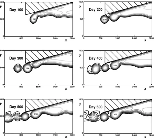
(ii) Sub-critical slant: The next angle,γ=15◦

, also proved difficult for some numerical

15

calculations. Because Φ remained close to unity for α≈1, our use of the viscosity

coefficient of 700 m2s−1led to unstable calculations. Nevertheless, for this angle, the situation was better than it was forγ=0◦

because, at least forα=1 (for which the theory

suggests a short detachment period), we saw the detachment of the first two eddies. Using a larger viscosity coefficient of 1000 m2s−1, and takeh0=0 after 200 d, we finally

20

obtained the detachment of two eddies, which formed a chain downstream (Fig. 6). Before the chain formation, however, the first detached eddy (shed after about 30 d) was absorbed by a second eddy that came from behind and propagated faster. This was followed by the splitting of the merged eddies into two.

We will see later that the absorption of the first eddy occurs whenγ is large. However,

25

in those cases, it ultimately results in a return of the first eddy into the retroflection area, which probably is connected with our hypothesis of restricted detachment. By contrast, for smallγ, the occasional capturing and splitting of eddies in the model was also found

(17)

OSD

5, 39–75, 2008

EGU

large viscosity coefficient. To check this further, we prolonged the calculation so that modeled time reached 700 d. We found that the occasional capturing and splitting of eddies continued. Nevertheless, the first two eddies ultimately left the generation area (despite the increasing effect of viscosity, which led to smoothing) and a chain of five eddies was displayed.

5

For h0=300 m, we obtained a somewhat different situation. The detached eddies formed a chain with no capturing; however, after an intense first eddy, the second one appeared to be much weaker, and sometimes it was hardly visible. This is possibly because intense (deeper) eddies are more strongly affected by frictional forces. Similar effects can be seen for lower starting values ofα, but the time of eddy development is,

10

as expected, longer. For example, whenα=0.4 and h0=0, the absorption of the first eddy by the second one occurs after about 200 d. Whenα=0.1, the first eddy is not

yet absorbed by day 200 but its development is almost over.

(iii) Near-critical slant: Simulations usingγ=30◦ and γ=45◦ gave eddies that were more variable than those in the caseγ=15◦

. This is despite the theoretical prediction

15

of a narrower range between the lower and upper boundaries. The first eddy was ab-sorbed only in our simulation forγ=45◦,α=1, and h0=0. The second one was absorbed in two simulations (with differenth0) forγ=30

◦

andα=1, when it was very weak. One

possible explanation for the variability lies in our use of the lower viscosity coefficient of 700 m2s−1(which, in that case, was sufficient to ensure stability). However, a more

20

important factor was that, despite relatively free detachment of the rings, they most often weakened gradually and, therefore, could not form a sufficiently stable chain. For a prolonged numerical simulation, the frequency of the ring capturing increased with time; as a result, after 700 d of simulation, only two rings went around the cape.

The radius of the first detached eddy increased only in our simulation for γ=30◦ ,

25

α=0.1, and h0=300 m, which could be an effect of the long period of detachment. In all other cases, the radii clearly decreased, especially forα=0.4 and α=1.0. This could

be one of the main factors responsible for maintaining the distances between the rings. It is difficult to say whether this effect was a consequence of the narrowing range of the

(18)

OSD

5, 39–75, 2008

Printer-friendly Version Interactive Discussion final radius, frictional forces, or both. In any case, we conclude that the possibility of an

eddy chain formation for such slants is questionable.

(iv) Super-critical slant: Simulations with a slant of 60◦, 75◦, and 90◦ clearly con-firmed the super-criticality because the possibility of detachment is severely limited. In some cases, such as that ofγ=60◦,α=1, and h0=300 m, we did not see a detachment

5

at all. Instead, a meander of relatively high, but variable, intensity appeared. Other simulations usingγ=75◦

,α=1, and h0=0, showed almost a complete damping of the first eddy, which remained stationary after its detachment. The most typical situation is shown in Fig. 7 (forγ=60◦

,α=1, and h0=0). After detachment, the first eddy gradually decayed before being recaptured by the meandering retroflected current behind. We

10

note that such a situation is similar to the behavior of rings detached from the retroflec-tion of the EAC, already described by Nilsson and Cresswell (1981), and Sokolov and Rintoul (2000). We can say, therefore, that, starting from γ=60◦

, the formation of a stable chain of eddies becomes impossible. To confirm this, we again extended our calculations, so that the modeled time reached 700 d. As a result, the absorbing

me-15

ander of the retroflected current was transformed into an eddy that was shed. However, later on, it was recaptured by the meander, just like the first detached eddy was. Such a process of shedding and recapturing repeated three times, and no eddies left the retroflection area. (The eddy shown in day 600 was later re-captured by day 700, but this recapturing is not displayed in Fig. 7.) In view of this, we suggest that, for such

20

values of the slant, recapturing becomes systematic and overwhelms the formation of eddies chain.

We should comment here about the situation whenα is small. Our simulations with α=0.1 and γ=60◦ and 75◦ qualitatively confirmed our theoretical prediction that the eddy cannot grow because theβ-induced force initially exceeds the combined force of

25

the currents (i.e., their long-shore momentum flux). In such cases, the plots showed the formation of a meander that was gradually forced into the wall. Its longitudinal dimension, along the wall, became much greater than the transverse one, negating our assumption of a nearly circular form. Eventually, an eddy of a smaller radius was

(19)

OSD

5, 39–75, 2008

EGU

formed from this meander. Further, the formed eddy continued decaying and exhibited almost no movement. We expected that it would finally be reabsorbed, but we did not reach that state.

4.3 Simulation-theory comparison

In addition to a qualitative analysis of ring behavior, we carried out a detailed

compar-5

ison of the theoretical modeling and the numerical simulations. (For this purpose, we used the magnified value ofβ.) The parameters that we compared are the eddy radius

at the moment of detachment,R_f, the eddy propagation velocity (C_ξ), and the ratio of the mass flux going into the eddies and the incoming flux (Φ).

Two introductory comments should be made here. First, Nof and Pichevin (2001, NP,

10

hereafter) carried out the quantitative comparison of the ratioq/Q as a function of time,

whereq is outgoing mass flux. In light of this, it was very important to take into account

the time evolution of the parameterα, which was dramatically altered by the viscosity

in the numerics. For us, it was inconvenient to conduct similar analysis because Φ was also variable in time, and we were operating mainly with its time-averaged values.

15

Therefore, we simplified our analysis by assuming that the value of Φ, averaged over the time of the numerical experiment, corresponded to the value ofα averaged in the

same way, and so did with the other parameters that we considered. Second, we also averaged the value ofC_ξ. Wherever possible, we used an averaging period between the moment of detachment and the last step in our experiment. However, in most

20

simulations with supercritical values ofγ, we were obliged to use a period between the

detachment and the re-absorption of the eddy.

According to NP, the coefficient α decreases quickly when its initial value is unity

and the outflow PV is zero. In the case of finite PV outflow,α decreases more slowly,

starting from about 0.22. Our situation was analogous when we started withα=1 and

25

α=0.4. However, in most of the experiments that started with α=0.1, we observed

a slight growth inα, especially for large γ. Most likely, this was a consequence of a

decrease in the size of the meander/eddy due to β. We only once obtained a very

(20)

OSD

5, 39–75, 2008

Printer-friendly Version Interactive Discussion slight decrease in α due to the combined effect of viscosity and a decreasing size.

Resulting from the above-mentioned behaviors ofα, its average value accumulated in

relatively narrow intervals: between 0.12 and 0.36 for h0=0, and between 0.08 and 0.33 forh0=300 m. The scattering weakened asγ was increased.

Figure 8 shows a comparison ofRf between the analytics and the numerical

simula-5

tions. Bearing in mind that the starting values ofα in the numerics were 1, 0.4, and 0.1,

we mark the numerical results for the time-averaged values ofα with circles and

dia-monds. Analyzing Fig. 8 a–c, whereγ is 0◦, 30◦and 60◦(respectively), we see that the numerical simulations confirm the theoretical tendency for the radius to decrease with growing angle. However, such a decrease is noticeably weaker than in the theoretical

10

prediction. In this connection, the scattering inRf also weakens withγ. For example, in

the caseh0=0 and starting fromα=0.1, 0.4, and 1.0, we obtained the values 381, 236, and 255 km forγ=0◦

(represented as diamonds in the upper panel) and 203, 181, and 213 km forγ=75◦(not shown). The theoretically predicted ranges, corresponding to the above-mentioned intervals, are between 240 and 350 km forγ=0◦

, and between 160

15

and 165 km forγ=75◦

. Strictly speaking, forγ=75◦

, we give here values corresponding to a greaterα. In our theory, we cannot calculate Rf corresponding to theα obtained

in the numerics whenγ is large, because under such conditions, the BE is forced into

the wall. The same situation caused the appearance of two numerical circles to the left of the theoretical curves in the lower plot (γ=60◦). We conclude that, for nonzero γ,

20

the numerical radii calculations give larger values than our theoretical model. However, the differences between the two are small. In the case of a zonal wall, the agreement is better overall, but the scattering of numerical values is significant.

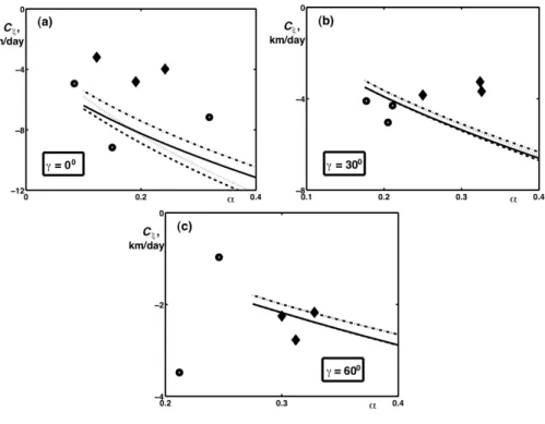
Figure 9 shows a comparison of the theoretical and numerical values ofCξforγ=0

◦ , 30◦, and 60◦ whereas Fig. 10 shows the comparison of Φ for the same angle. We

25

note that there are two circles instead of three in the lower panel of Fig. 9. This is because, as mentioned, in our simulation withγ=60◦,α=1 and h0=300 m we did not achieve detachment, so we could not compute the eddy drift velocity. On the whole, the agreement is satisfactory. Concerning Cξ, we can say that this agreement obviously

(21)

OSD

5, 39–75, 2008

EGU

improves with growing angleγ for h0=0, and in the case ofh0=300 m, it looks slightly worse because of the noticeable scattering in the numerical values. Most importantly, the agreement of the theoretical and numerical eddy drift velocity confirms (3) which was introduced without any rigorous analysis.

The agreement seems to be worse with regard to Φ, especially for nonzeroγ.

How-5

ever, it is not easy to compute the mass flux numerically because of noise (e.g., in the forms of Kelvin waves and secondary meandering of the outgoing flow, and frictional effects) leading to ambiguity in the boundaries of this flux. The scattering of the numer-ical values ranges between slightly negative and about 0.18, which is admissible when the theoretical values are between zero and 0.15 (forγ=30◦

), or even between zero and

10

0.04 (forγ=60◦). In either case, the numerics clearly confirm that Φ is considerably smaller when the coastline is highly slanted.

5 Summary and conclusions

The main aim of our theoretical and numerical analyses was to examine the hypothesis that the glacial AC was similar to the present day EAC where, due to the orientation of

15

the coastline, no mean rings shedding is usually observed. According to our hypothe-sis, the shedding of eddies is severely restricted when the slant angleγ is greater than

65◦ (the present EAC, and the glacial AC) but occurs steadily when γ is smaller than

about 20◦(present AC).

To examine this hypothesis we developed a non-linear model of retroflecting currents

20

that flow along slanted coastlines. We studied the dependence of rings diameter, speed and frequency of shedding, on the coastline slant, the PV of the formed eddies, and the thickness of the surrounding upper layer. The results are shown in Figs. 3–5 illustrating that there is significant shedding when the slant is small (sub-critical angle) but almost no shedding when the slant is large (supercritical angle).

25

Although we do not give an exact definition of the critical angle, we treated the angle of visible convergence of the lower and upper boundaries of the theoretical eddy radius

(22)

OSD

5, 39–75, 2008

Printer-friendly Version Interactive Discussion (Fig. 3) as the critical angle. Indeed, according to our definition of the lower boundary

(osculating rings), the convergence of the lower and upper boundaries means that a chain of detached rings must form downstream. This implies that, in practice, the rings are likely to hinder each other owing, for instance, to viscosity. Because for supercritical slants, small long-shore drift speeds are predicted for detached rings,

5

the slowly moving eddy will be hindered and recaptured by the one behind it or by a meander of the retroflected current. Such a scenario agrees well with the dynamics retroflected current EAC rings described by Nilsson and Cresswell (1981), and Sokolov and Rintoul (2000). These rings usually stay at the same place for a long time and may eventually re-coalesce with the EAC.

10

We used a modified version of the Bleck and Boudra (1986) reduced gravity isopycnic model and obtained plots surprisingly similar to the observed EAC dynamics when the slant was taken to be 60◦ or more (Fig. 7). Also, as expected, we obtained chains of detached eddies when the slant was 15◦ (Fig. 6) and, a less clear chain whenγ=30◦. The transition range of slant angles was between 35◦ and 55◦, which agrees with our

15

description of the critical angle that is approximately 20◦, 40◦, 60◦, and 65◦ whenα is

0.1, 0.2, 0.5, and unity (respectively). During most of our simulation,α was between

0.15 and 0.3 and the variables obtained in the theoretical modeling were in quantitative agreement with our numerical simulations (Figs. 8–10). On this basis, we suggest that the significant reduction in the exchange between the Indian and South Atlantic

20

Oceans during the glacials and the YD was due to a northward migration of the WSC. This led the AC retroflection area to shift to a latitude of a supercritical coastal slant (Fig. 1). Other important results of our study can be summarized as follows:

– An increase in γ leads to a decrease in the radii of detached rings and makes

them less sensitive to variations inα (Fig. 3). Nevertheless, even in the case of

25

supercritical slant, the theoretical values ofR_f are 200–220 km and, therefore, still noticeably greater than the observational values.

(23)

OSD

5, 39–75, 2008

EGU

(Fig. 5). When γ≥6◦, it becomes less than unity (even for eddies with zero PV, i.e., intense eddies) implying that the “vorticity paradox” discussed by ZN is cir-cumvented.

– Our assumption of a nearly circular BE fails when the PV is large (weak eddies)

andγ is not very small. In that case, the BE does not grow; rather, it is forced into

5

the wall and deforms.

Concerning the distance between two consecutive eddies, we note that the ratio

Rf u/Rf l is maximal in the case of zonal wall, when it is approximately 1.11 (i.e., less

than 21/5). Therefore, we conclude that, theoretically, the separation distance should not exceed the eddy diameter. This conclusion is not far from the observational data,

10

even though the eddy diameter is smaller than our theory yields. Indeed, if the eddies are shed on average 5 times per year, and their migration rate varies between 2 and 10 cm/s, then, during the period of generation, the eddy migrates 380 km on average, and at the most 630 km. Taking into account a typical eddy radius of 140 km, we obtain that the ratio (d /2R) is 0.36 in average, with a maximal value of 1.25.

15

As is frequently the case, our ability to compare our theoretical results with the nu-merical simulations was limited due to the effect of viscosity in the numerics, which led to a relatively narrow range ofα. In addition, the viscosity in the numerics makes

the outgoing flux appear blurry, resulting in a possibility of errors as large as 0.2 in the determination of Φ. Despite both of these aspects, our comparison is very useful.

20

Although in our numerical simulations we confirmed the observation that capturing and re-splitting of eddies can be a possible cause of non-regularity in their shedding (Veld-hoven, 2005), we find that non-regularity could also be connected with variability of the retroflection position (Lutjeharms, 2006). For example, we note that Esper et al. (2004) pointed out seasonality of its position.

25

Our results also agree with Chassignet and Boudra’s (1988) sensitivity analysis, which showed that decreasing coastal slant leads to an increase in the production of rings. On the other hand, the numerical experiments by Pichevin et al. (1999) showed

(24)

OSD

5, 39–75, 2008

Printer-friendly Version Interactive Discussion that the dependence of the periodicity of rings shedding on the slant angle could be

negligible. This might be a result of the specific geometry of coastline in their model. We leave this issue as a subject for future investigations. Finally, we note that taking into account the coastline slant could also improve understanding of other retroflecting oceanic currents such as the North Brazil Current (NBC). Unfortunately, the question

5

of a priori determination of the eddy PV remains unanswered, and this is significant particularly when the vorticity of the incoming fluid is cyclonic rather than anticyclonic.

Appendix A List of symbols

AC – Agulhas Current

BE – basic eddy

Cx – eddy velocity in the open ocean

C_ξ – eddy migration rate along the slanted coast

Cξf – eddy migration rate after detachment

Cξl, Cξu – values ofCξf for eddies with radiiRf l, Rf u, respectively d – distance between consecutive eddies

d_u – “upper” boundary ofd

EAC – East Australian Current

g′ – reduced gravity

h0 – upper layer thickness at the wall

H – upper layer thickness outside the retroflection area

Hf l, Hf u – values ofH at the moments tf l, tf u, respectively

LGM – Last Glacial Maximum

MOC – meridional overturning circulation NADW – North Atlantic Deep Water

NP – Nof and Pichevin (2001) PV – potential vorticity

(25)

OSD

5, 39–75, 2008

EGU Q – mass flux of the incoming current

q – mass flux of the retroflected current

R – radius of the eddy (a function of time)

Ri – initial radius of the eddy R_f – radius of detached eddy

R_{f l}, R_{f u} – “lower” and “upper” boundaries ofR_f

t – time

t_f – period of the eddies generation

t_{f l}, t_{f u} – “lower” and “upper” boundaries oft_f

WSC – wind stress curl

YD – Younger Dryas

ZN – Zharkov and Nof, paper submitted to “Ocean Sciences”

α – vorticity (twice the Rossby number)

β – meridional gradient of the Coriolis parameter

γ – slant of coastline

ξ,η – axes of rotated moving coordinate system

Φ _– _{ratio of mass flux going into the eddies and incoming mass flux} Φ_l_{, Φ}_u _– _{values of Φ for eddies with radii}_R_{f l}_{, R}_{f u}_{, respectively}

Acknowledgements. The study was supported by the NASA under the Earth System Science

Fellowship Grant NNG05GP65H. V. Zharkov was also funded by the J. and S. O’Brien Grad-uate Fellowship. We are grateful to S. van Gorder for helping in the numerical simulations, to D. Samaan for helping in preparation of manuscript, and to J. Beall for helping in improving the

5

style.

(26)

OSD

5, 39–75, 2008

References

Andrews, J. C. and Scully-Power, P.: The structure of an East Australian Current anticyclonic eddy, J. Phys. Oceanogr., 6, 756–765, 1976.

Arruda, W. Z., Nof,D., and O’Brien, J. J.: Does the Ulleung eddy owe its existence toβ and

nonlinearities?, Deep-Sea Res., 51, 2073–2090, 2004.

5

Bard, E.: Climate shock: abrupt changes over millennial time scales, Phys. Today, 55, 32–38, 2002.

Berger, W. H. and Wefer, G.: Expeditions into the past: paleoceanographic studies in the South Atlantic, Springer-Verlag, Berlin-Heidelberg, 35–156, 1996.

Bleck, R. and Boudra, D.: Wind-driven spin-up in eddy resolving ocean models formulated in

10

isopycnic and isobaric coordinates, J. Geophys. Res., 91, 7611–7621, 1986.

Bostock, H. C., Opdyke, B. N., Gagan, M. K., Kiss, A. E., and Fifield, L. K.: Glacial/interglacial changes in the East Australian current, Clim. Dynam., 26, 645–659, 2006.

Burne, A. D., Gordon, A. L., and Haxby, W. F.: Agulhas eddies: A synoptic view using geosat ERM data, J. Phys. Oceanogr., 25, 902–917, 1995.

15

Chassignet, E. P. and Boudra, D. B.: Dynamics of the Agulhas retroflection and ring formation in a numerical model, II. Energetics and ring formation, J. Phys. Oceanogr., 18, 304–319, 1988.

de Ruijter, W. P. M.: Asymptotic analysis of the Agulhas and Brazil Current systems, J. Phys. Oceanogr., 12, 361–373, 1982.

20

de Ruijter, W. P. M., Biastoch, A., Drijfhout, S. S., Lutjeharms, J. R. E., Matano, R. P., Pichevin, T., van Leeuwen, P. J., and Wejer, W.: Indian-Atlantic interocean exchange: Dynamics, esti-mation and impact, J. Geophys. Res., 104, 20 885–20 910, 1999.

Esper, O., Versteegh, G. J. M., Zonneveld, K. A. F., and Willems, H.: A palynological recon-struction of the Agulhas Retroflection (South Atlantic Ocean) during the Late Quaternary,

25

Global Planet. Change, 41, 31–62, 2004.

Gasse, F.: Hydrological changes in the African tropics since the Last Glacial Maximum, Qua-ternary Sci. Rev., 19, 189–211, 2000.

Goni, G. J., Garzoli, S. L., Roubicek, A. J., Olson, D. B., and Brown, O. B.: Agulhas ring dynamics from TOPEX/POSEIDON satellite altimeter data, J. Mar. Res., 55, 861–883, 1997.

30

Gordon, A. L., Lutjeharms, J. R. E., and Gr ¨undlingh, M. L.: Stratification and circulation at the Agulhas Retroflection, Deep-Sea Res., 34, 565–599, 1987.

(27)

OSD

5, 39–75, 2008

EGU

Howard, W. R. and Prell, W. L.: Late quaternary surface circulation of the southern Indian Ocean and its relationship to orbital variation, Paleoceanography, 7, 79–117, 1992.

Kawagata, S.: Tasman front shifts and associated paleoceanographic changes during the last 250 000 years: foraminiferal evidence from the Lord Howe Rise, Mar. Micropaleontol, 41, 167–191, 2001.

5

Knorr, G. and Lohmann, G.: Southern Ocean origin for the resumption of the Atlantic overturn-ing circulation duroverturn-ing deglaciation, Nature, 424, 532–536, 2003.

Lutjeharms, J. R. E.: The exchange of water between the South Indian and South Atlantic Oceans, in: The South Atlantic: Present and Past Circulation, edited by: Wefer, G., Berger, W., and Sielder, G., Springer-Verlag, Berlin-Heidelberg, 125–162, 1996.

10

Lutjeharms, J. R. E.: The Agulhas Current, Sprinter-Verlag, Berlin-Heidelberg-New York, XIV, 330 pp., 2006.

Martinez, J. I.: Late Pleistocene palaeoceanography of the Tasman Sea: implications for the dynamics of the warm pool in the western Pacific, Palaeogreogr. Palaeoecl., 112, 19–62, 1994.

15

Martinez, J. I., de Deckker, P., and Barrows, T.T.: Palaeoceanography of the western Pacific warm pool during the last glacial maximum: long-term climatic monitoring of the maritime continent, in: Bridging Wallace’s line, edited by: Kershaw, P., Bruno, D., Tapper, N., Penny, D., and Brown, J., Adv. Geoecol., 34, 147–172, 2002.

Nilsson, C. S., Andrews, J.C., and Scully-Power, P.: Observation of eddy formation off East

20

Australia, J. Phys. Oceanogr., 7, 659–669, 1977.

Nilsson, C. S. and Cresswell, G. R.: The formation and evolution of East Australian Current warm-core eddies, Prog. Oceanogr., 9, 133–183., 1981.

Nof, D.: On the migration of isolated eddies with application to Gulf Stream rings, J. Mar. Res., 41, 399–425, 1983.

25

Nof, D.: The momentum imbalance paradox revisited, J. Phys. Oceanogr., 35, 1928–1939, 2005.

Nof, D. and Pichevin, T.: The ballooning of outflows, J. Phys. Oceanogr., 31, 3045–3058, 2001. Nof, D. and van Gorder, S.: Did an open Panama Isthmus correspond to an invasion of Pacific

water into the Atlantic, J. Phys. Oceanogr., 33, 1324–1336, 2003.

30

Peeters, F. J. C., Acheson, R., Brummer, G. J. A., de Ruijter, W. P. M., Schneider, R. R., Ganssen, G. M., Ufkes, E., and Kroon, D.: Vigorous exchange between the Indian and Atlantic oceans at the end of the past five glacial periods, Nature, 430, 661–665, 2004.

(28)

OSD

5, 39–75, 2008

Pichevin, T., Nof, D., and Lutjeharms, J. R. E.: Why are there Agulhas Rings?, J. Phys. Oceanogr., 29, 693–707, 1999.

Rau, A. G., Rogers, J., Lutjeharms, J.R.E., Giraudeau, J., Lee-Thorp, J. A., Chen, M.-T., and Waelbroeck, C.: A 450-ky records of hydrological conditions on the western Agulhas Bank Slope, south of Africa, Mar. Geol., 180, 183–201, 2002.

5

Schouten, M. W., de Ruijter, W. P. M., van Leeuwen, P. J., and Lutjeharms, J. R. E.: Translation, decay and splitting of Agulhas rings in the south-eastern Atlantic ocean, J. Geophys. Res., 105, 21 913–21 925, 2000.

Schouten, M. W., de Ruijter, W. P. M., and van Leeuwen, P. J.: Upstream control of the Agulhas ring shedding, J. Geophys. Res., 107(C8), 10.1029/2001JC000804, 2002.

10

Shi, C. and Nof, D.: The destruction of lenses and generation of wodons, J. Phys. Oceanogr., 24, 1120–1136, 1994.

Sokolov, S. and Rintoul, S.: Circulation and water masses of the southwest Pacific: WOCE Section P11, Papua New Guinea to Tasmania, J. Mar. Res., 58, 223–268, 2000.

Speich, S., Lutjeharms, J. R. E., Penven, P., and Blanke, B.: Role of bathymetry

15

in Agulhas Current configuration and behavior, Geophys. Res. Lett., 33, L23611, doi:10.1029/2006GL027157, 2006.

Tilburg, C. E., Hulburt, H. E., O’Brien, J. J., and Shriver, J. F.: The dynamics of the east Australian current system: the Tasman front, the east Auckland current and the East Cape current, J. Phys. Oceanogr., 31, 2917–2943, 2001.

20

van Veldhoven, A. K.: Observations of the evolution of Agulhas Rings. Proefschrift ter verkri-jging van de graad van doctor aan de Universiteit Utrecht op gezag van de Rector Magnificus Prof. Dr. W.H. Gispen, Nederlands, 166 pp., 2005.

Weijer, W., de Ruijter, W. P. M., and Dijkstra, H. A.: Stability of the Atlantic overturning circula-tion: Competition between Bering Strait freshwater flux and Agulhas heat and salt sources,

25

J. Phys. Oceanogr., 31, 2385–2402, 2001.

Weijer, W., de Ruijter, W. P. M., Dijkstra, H. A., and van Leeuwen, P. J.: Impact of interbasin exchange on the Atlantic Overturning Circulation, J. Phys. Oceanogr., 29, 2266–2284, 1999. Zharkov, V. and Nof, D.: Retroflection from slanted coastlines–circumventing the “vorticity

para-dox”, Ocean Sci. Discuss., 5, 1–37, 2008,

30

(29)

OSD

5, 39–75, 2008

EGU

Fig. 1. Schematic diagram of the Agulhas retroflection and the detached rings. Note that

the slant of the coastline relative to the meridional direction varies dramatically as one moves northward along the coast. Box I displays glacial conditions: wind stress curl vanished at the lower latitudes where the coastal slant is about 60◦. Ring shedding was rare because the translation velocity of the detached rings along the wall was small. Some rings could be dissipated or reabsorbed by the meandering current. Box II displays post-glacial conditions: wind stress curl vanishes at higher latitudes where the coastal slant is about 20◦. A chain of rings is regularly shed because the migration speed along the wall is high.

(30)

OSD

5, 39–75, 2008

Printer-friendly Version Interactive Discussion EGU = t R t

)

Fig. 2. Geometries associated with the lower and upper boundaries of the final eddy radius.

The upper panel (a) shows two consecutive osculating eddies (d =0) away from the

retroflec-tion. The detachment periodt_{f l} is obtained by a division of the doubled-finaleddy- radius, 2R_{f l}, by the modulus of the final eddy migration rate. The segment BC corresponds to the western boundary of the integration area (see ZN). The lower panel (b) shows the already detached eddy (centered in E₁) migrating at the rate −C_ξ(t) , and an incipient basic eddy (BE) centered

in E. At the moment t_{f u}, the distance between the two eddies is (R_{f u}−R_i), which is positive because the incipient BE is less developed. Therefore, our ABCD contour encloses only the incipient BE.

(31)

OSD

5, 39–75, 2008

Printer-friendly Version Interactive Discussion EGU 5 6 R 450 _R ₇₅0 0 1

Fig. 3. The theoretical solutions. (a)R_{f l} (solid lines) and R_{f u} (dashed lines) plotted against the angleγ. Each pair of convergent curves is marked by a corresponding value of α. (b) R_{f l} (solid lines), R_{f u} (dashed lines), and R_i (dash-and-dotted line) plotted against α. Each

pair of divergent curves is marked by a corresponding value ofγ. It is seen that the curves

corresponding toγ≥45◦

start from the curve of R_i . Note that lines depictingR_{f l} andR_{f u} for

γ=75◦

almost coincide. Also, note that, as should be the case, the upper boundary is always above the lower boundary. In both plots:h0=0,β=2.3×10

−11

m−1s−1.