en fr

HAL Id: tel-00069125

https://tel.archives-ouvertes.fr/tel-00069125

Submitted on 16 May 2006

HAL is a multi-disciplinary open access archive for the deposit and dissemination of sci-entific research documents, whether they are pub-lished or not. The documents may come from teaching and research institutions in France or abroad, or from public or private research centers.

L’archive ouverte pluridisciplinaire HAL, est destinée au dépôt et à la diffusion de documents scientifiques de niveau recherche, publiés ou non, émanant des établissements d’enseignement et de recherche français ou étrangers, des laboratoires publics ou privés.

phenomena in neuronal networks

Roberta Sirovich

To cite this version:

Roberta Sirovich. Mathematical models for the study of synchronization phenomena in neuronal networks. Neurons and Cognition [q-bio.NC]. Université Joseph-Fourier - Grenoble I, 2006. English. �tel-00069125�

Mathematical models

for the study of synchronization phenomena

in neuronal networks

Mod`eles math´ematiques

pour l’ ´etude des ph´enom`enes de synchronisation dans les r´eseaux neuronaux

Th`

ese de doctorat

pr´esent´ee `a

l’ Universit`a degli Studi di Torino et l’ Universit´e Grenoble I Joseph Fourier par

Roberta Sirovich

Jury

Prof. Ferdinando Arzarello, Pr´esident Prof. Petr L´ansk´y, Rapporteur Prof. Jean-Pierre Rospars, Rapporteur Prof. Laura Sacerdote, Codirecteur de th`ese Prof. Alessandro E. P. Villa, Codirecteur de th`ese

Dr. Patricia Duchamp-Viret, Expert

Mathematical models

for the study of synchronization phenomena

in neuronal networks

Roberta Sirovich

Dipartimento di Matematica, Universit`a degli Studi di Torino

Laboratoire de Neurosciences Pr´ecliniques – INSERM U318, Universit´e Grenoble 1

The spike train, i.e. the sequence of the action potential timings of a single unit (i.e. a single neuron in most cases), is the usual data that is analyzed in electrophysiological record-ings for the description of the firing pattern which is supposed to characterize a certain type of cell. The statistical distribution of the interspike intervals (ISI) is a first order statistics that is often provided in experimental studies. However, its interpretation is far from being trivial and could reveal interesting phenomena associated to the underlying network activity. We present the results obtained describing the firing activity of a small network of neurons with a mathematical jump diffusion model. That is the membrane potential as a function of time is given by the sum of a stochastic diffusion process and two counting processes that provoke jumps of constant sizes at discrete random times. Different distributions are consid-ered for such processes: jump processes with inter-events Exponentially and Inverse Gaussian distributed, Wiener and Ornstein Uhlenbeck diffusion processes. Moreover we consider two configuration of the small network: open circuit and close circuit. Two main results emerge. The first one is that interspike intervals (ISI) histograms show more than one peak (multi-modality) and exhibit a resonant like behavior. This fact suggests that in correspondence of each mode (i.e. the lag of the maxima) the cell has a higher probability of firing such that the the lags become characteristic times of the cell which could be modulated under physiological conditions. The second main result concerns the role of inhibition in neuronal coding. Indeed we show that the inhibitory inputs may facilitate the transmission of the spikes generated by the excitatory unit. This fact suggests that inhibitory cells are not only involved in keeping balanced the excitability of the cell but that they may also play a key role in the information process.

The simulation of such kind of models requires to evaluate the first passage time through a threshold of a stochastic process. In this framework arises the necessity to improve classical algorithms with the evaluation of bridge process crossing probabilities. So that the second

processes associated to a regular diffusion process. The SDE fulfilled by the conditioned process is written, starting from the SDE giving the process on which the bridge is built. Two methods to have a version of the solution of the SDE giving the bridge are explored, i.e. the space time transformations and the conditioning of the solution of a suitable second order SDE with Dirichlet boundary conditions.

Mod`

eles math´

ematiques

pour l’ ´

etude des ph´

enom`

enes de synchronisation

dans les r´

eseaux neuronaux

Roberta Sirovich

Dipartimento di Matematica, Universit`a degli Studi di Torino

Laboratoire de Neurosciences Pr´ecliniques – INSERM U318, Universit´e Grenoble 1

Les enregistrements ´electrophysiologiques extracellulaires permettent d’obtenir le soi-disant “train de spikes”, c’est `a dire la s´erie temporelle des potentiels d’action d’un neurone, qui est suppos´ee ˆetre l’une des caract´eristiques fonctionnelles de l’activit´e neuronale. La dis-tribution des intervalles entre deux d´echarges neuronales successives (ISI) est une statistique du premier ordre couramment utilis´ee dans les ´etudes exp´erimentales ´electrophysiologiques. Cependant, son interpr´etation est loin d’ˆetre banale et pourrait indiquer des ph´enom`enes int´eressants associ´es `a l’activit´e fondamentale du r´eseau. Afin de mieux comprendre cette statistique, ce travail pr´esente les r´esultats obtenus par l’´etude de l’activit´e d’un micro r´eseau neuronal d´ecrit par des ´equations math´ematiques du type “saut-diffusion”. La variation du potentiel membranaire du neurone en fonction du temps est donn´e par la somme d’un processus stochastique de diffusion et de deux processus de point, qui provoquent des sauts d’amplitude constante `a des temps al´eatoires discrets. Diff´erentes distributions sont con-sid´er´ees pour ces processus: processus de saut avec inter-´ev´enements distribu´es exponentielle-ment ou par une fonction gaussienne inverse, processus de diffusion de Wiener ou d’Ornstein Uhlenbeck. Nous consid´erons aussi deux configurations de micro r´eseau: r´eseau ouvert ou r´eseau ferm´e, c’est `a dire avec r´etroaction du processus r´esultant sur les processus g´en´erateurs. Ce travail fait ressortir deux r´esultats principaux. Le premier est que les histogrammes des ISI montrent plusieurs maxima et un comportement de type r´esonnant. En correspondance de chaque maximum la cellule a une probabilit´e plus ´elev´ee de se d´echarger, de mani`ere que les latences des pics d’histogrammes repr´esentent des temps caract´eristiques de la cellule pouvant ˆetre modul´es par diverses conditions physiologiques. Le deuxi`eme r´esultat principal concerne le rˆole de l’inhibition dans le codage neuronal. Nous avons d´emontr´e que, sous certaines conditions, les aff´erences inhibitrices peuvent faciliter la transmission des potentiels d’action propag´es par les connexions excitatrices. De ce fait l’on d´eduit que les cellules inhibitrices ne doivent pas seulement ˆetre consid´er´ees pour leur rˆole ´equilibreur vis-`a-vis de l’excitabilit´e

et le codage de l’information neuronale.

La simulation de ce type de mod`eles exige l’´evaluation du temps de premier passage par le seuil d’un processus stochastique. Dans ce cadre surgit la n´ecessit´e d’am´eliorer les algorithmes classiques avec l’´evaluation des probabilit´es de croisement du seuil par un processus “bridge”, correspondant au processus de diffusion simul´e. La deuxi`eme partie de ce manuscrit est d´edi´ee `

a une ´etude purement th´eorique sur les processus bridge multidimensionnels associ´es `a un processus de diffusion r´egulier. Nous ´ecrivons l’´equation stochastique diff´erentielle satisfaite par le processus bridge et proposons deux m´ethodes alternatives pour trouver une version de la solution dans le cas bidimensionnel. Toutes les m´ethodes pr´esent´ees sont illustr´ees avec l’exemple du processus du mouvement brownien int´egr´e.

Publications

[1 ] M. T. Giraudo, L. Sacerdote and R. Sirovich Effects of random jumps on a very simple neuronal diffusion model. BioSystems, 67 (2002), pp. 74-83.

[2 ] L. Sacerdote and R. Sirovich A Wiener process with Inverse Gaussian time distributed jumps as a model for neuronal activity. Proceedings of the 5th ESMTB Conference 2002, V.Capasso Editor.

[3 ] L. Sacerdote and R. Sirovich Multimodality of the Interspike Interval Dis-tribution in a simple jump-diffusion model. Scientiae Mathematicae Japonicae, 8 (2003), pp. 359-374.

[4 ] R. Sirovich and L. Sacerdote Noise induced phenomena in jump diffusion models for single neuron spike activity. IJCNN2004 CD-ROM Conference Proceed-ings, IEEE Catalog Number 04CH37541C, ISBN: 0-7803-8360-5.

[5 ] R. Sirovich, L. Sacerdote and A.E.P. Villa Multimodal inter-spike interval distribution in a jump-diffusion neuronal model. Submitted for publication.

[6 ] R. Sirovich and C. Zucca Multidimensional Bridges with application to the Integrated Brownian Motion. Preprint.

Adresses

Pr´esident

Prof. Ferdinando Arzarello

Dipartimento di Matematica, Universit`a degli studi di Torino Via Carlo Alberto 10

10128 Torino, Italia. Rapporteur Prof. Petr L´ansk´y

Institute of Physiology, Academy of Sciences of the Czech Republic Videnska 1083

142 20 Prague 4, Czech Republic. Rapporteur

Prof. Jean-Pierre Rospars

INRA - Unit`e de Phytopharmacie et M´ediateurs Chimiques Route de St-Cyr

F-78026 Versailles cedex, France. Codirecteur de Th`ese

Prof. ssa Laura Sacerdote

Dipartimento di Matematica, Universit`a degli studi di Torino Via Carlo Alberto 10

10128 Torino, Italia. Codirecteur de Th`ese Prof. Alessandro E. P. Villa

Inserm U318, Laboratoire de Neurosciences Pr´ecliniques Universit`e Joseph Fourier

BP 217 38043 Grenoble cedex 9, France. Expert

Dr. ssa Patricia Duchamp-Viret

Laboratoire de Neurosciences et Syst´emes Sensoriels Universit`e Claude Bernard

50, avenue Tony Garnier F-69366 Lyon cedex 07.

R´

ESUM´

E

Comprendre le fonctionnement du cerveau est l’un des d´efis scientifiques les plus importants. Jusqu’`a la fin du XIX`eme si`ecle, et au d´ebut du XX`eme, les scientifiques n’´etaient pas encore persuad´es que le tissu c´er´ebral ´etait compos´es par des cellules. C’est le scientifique espag-nol Santiago Ram´on y Cajal, avec son remarquable travail histologique, qui convainquit la communaut´e scientifique que le cerveau ´etait constitu´e par des cellules, les neurones, qui sont de v´eritables ´el´ements unitaires et qui agissent l’un sur l’autre par des contacts sp´ecialis´es appel´es synapses. Aujourd’hui nous savons que le tissu du cerveau se compose de deux types principaux de cellules, les cellules nerveuses, appel´ees neurones, et les cellules neurogliales, appel´ees g´en´eralement glie. La glie joue un rˆole important, pas encore compl`etement com-pris, mais qui ne fait pas l’objet de cette ´etude. L’unit´e qui nous int´eresse et qui traite principalement la transmission du signal, est le neurone. Mais qu’est-ce que c’est un signal?

Dynamique de la membrane neuronale

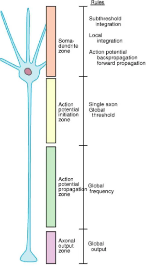
Dans le syst`eme nerveux humain il est possible de trouver pr`es de 1012 neurones car-act´eris´es par une diversit´e morphologique et fonctionnelle extraordinaire. Cependant, comme point de d´epart, nous allons d´ecrire une cellule neuronale typique, et simplifi´ee, (cf. Figure 0.1), avec trois ´el´ements fondamentaux: le corps de la cellule, appel´e soma, qui est la partie de la cellule o`u se trouve le noyau; les dendrites, qui sont des appendices ramifi´ees donnant lieu `a l’arbre dendritique, et o`u se produisent les contacts avec les autres cellules aux emplacements sp´ecialis´es appel´es synapses; l’axone qui est une appendice particuli`ere et unique, avec des branchements terminaux, par laquelle se propage le potentiel d’action. Il y a une diff´erence de potentiel entre l’int´erieur et l’ext´erieur de la cellule neuronale, mais ce qui caract´erise un neurone est son excitabilit´e. Le courant ´electrique est port´e par des ions, principalement le

sodium (Na), le potassium (K), le calcium (Ca) et le chlorure (Cl), qui traversent la mem-brane cellulaire dans certaines conditions. Mˆeme si les lois de la physique qui r`eglent les mouvements ioniques sont simples, les propri´et´es ´electrophysiologiques caract´eristiques d’une cellule neuronale sont tr`es complexes. La description analytique de la d´echarge d’une

cel-Figure 0.1. Repr´esentation sch´ematique d’une cellule neuronale typique.

lule neuronale porta A. L. Hodgkin et A. F. Huxley [24] `a formuler les premi`eres ´equations en fonction de la concentration diff´erentielle des conductances ioniques et des concentrations des ions. La membrane du neurone peut ˆetre vue comme une s´erie de capacit´es ´electriques (dues `a la double couche lipidique de la membrane cellulaire) et de r´esistances variables (dues aux canaux ioniques). Une interpr´etation simplifi´ee de cette vue porta `a la formulation des mod`eles stochastiques `a partir du mod`ele de Lapique et qui seront trait´es en d´etail dans le chapitre 2. Dans ce type de mod`eles, `a chaque fois que le potentiel de membrane atteint un ´etat particulier, le neurone produit un potentiel d’action, appel´e spike. Cet ´etat particulier

CONNECTIVIT´E NEURONALE xiii est souvent repr´esent´e par un seuil du potentiel de membrane: c’est une mani`ere tr`es prag-matique et pratique de traiter le probl`eme mais ce n’est pas une description physiologique des processus biophysiques qui r`eglent la g´en´eration d’un spike.

Une autre approche du probl`eme consiste en une approche ph´enom´enologique qui est trait´ee computationellement par des mod`eles num´eriques digitaux, plutˆot que analytique-ment. Cette approche s’appuie sur des mod`eles neuronaux simplifi´es appel´es int´egrateurs tout-ou-rien (en anglais: integrate-and-fire) est s’est d´evelopp´ee `a partir du travail de Mc Cullock et Pitts (1943) pour la simulation de r´eseaux neuronaux de grande taille.

Les deux approches ont chacune le pour et le contre et nous pr´esentons dans cette th`ese quelques id´ees qui pourraient repr´esenter un compromis dans le sens que les formulations discr´etis´ees des mod`eles analytiques pourraient ˆetre employ´ees pour des simulations digitales intensives.

Connectivit´e neuronale

Le potentiel d’action est produit dans une zone particuli`ere de la membrane cellulaire, la partie initiale de l’axone (cf. Fig. 0.1), et il est transmis dans toutes les branches de l’axone. Les points d’interaction entre deux neurones, les synapses, sont orient´es de sorte que l’on diff´erencie le neurone pr´esynaptique (en anglais: le neurone trigger) et le neurone postsy-naptique (en anglais: le neurone follower). Quand le potentiel d’action atteint la synapse, le neurone pr´esynaptique lib`ere un neurotransmetteur chimique qui traverse la fente synaptique et atteint la membrane du neurone postsynaptique o`u il se lie avec des r´ecepteurs sp´ecifiques. Il y a plusieurs genres de r´ecepteurs (ionique, metabotropique, etc...) qui sont caract´eris´es par des temps d’activation allant de la milliseconde jusqu’`a plusieurs secondes, par divers niveaux de plasticit´e et par divers effets de polarisation sur la membrane postsynaptique. L’effet de polarisation permet de distinguer les neurones en deux cat´egories principales: ex-citateur (si un courant de d´epolarisation, EPSP, est produit) et inhibiteur (si un courant d’hyperpolarisation, IPSP, est produit).

Train de spikes

Ce travail aborde l’´etude du syst`eme nerveux par le biais de mod`eles qui g´en`erent des trains de spike. Le train de spike est la sequence temporelle des potentiels d’action produits par une seule unit´e, habituellement un neurone. Les techniques exp´erimentales r´ecentes ont ´evolu´e vers l’enregistrement de l’activit´e neuronale par des ´electrodes multiples permettant d’obtenir des s´eries temporelles multivari´ees correspondant aux trains de spike provenants de plusieurs cellules enregistr´ees simultan´ement. La r´ep´etition de ISI particuliers, au del`a de la chance estim´ee du hasard, observ´ee dans les trains de spike [3], [6], [63], [64] soul`eve plusieurs questions sur la signification que pourraient avoir de tels motifs temporels (en anglais: pattern) soit en rapport avec des motifs sp´ecifiques d’activit´e neuronale au sein d’un r´eseau soit avec des propri´et´es intrins`eques propres `a la membrane des cellules analys´ees.

Cadre du mod`ele adopt´e

Une sous-classe de pattern temporels, indiqu´ee par les histogrammes multimodaux de la distribution des ISI, peut ˆetre ´etudi´ee en d´etail avec l’aide de mod`eles math´ematiques de la dynamique neuronale. C’est l’approche que nous avons adopt´e dans cette ´etude. Le point de d´epart ont ´et´e les mod`eles stochastiques de saut-diffusion. Ce type de mod`eles d´ecrit le potentiel de membrane `a l’aide d’un processus de diffusion et de la somme de deux processus de point qui provoquent des sauts d’amplitude constante `a des temps al´eatoires discrets. En particulier nous avons ´etudi´e les deux mod`eles suivants (illustr´es en d´etail dans le chapitre 2):

1. processus de diffusion de Wiener avec sauts;

2. processus de diffusion d’Ornstein Uhlenbeck avec sauts. Structure de la dissertation

Le chapitre 1 introduit ce document, qui est divis´e en deux sections. La premi`ere section (qui comprend les chapitres de 2 `a 5) d´efinit les fondements math´ematiques des mod`eles neuromim´etiques ainsi que les algorithmes utilis´es pour leur simulation et pour les analyses des r´esultats computationnels. La deuxi`eme section (chapitre 6) introduit et d´ecrit en d´etail les r´esultats originaux obtenus dans la recherche purement math´ematique des processus de

STRUCTURE DE LA DISSERTATION xv type “bridge”. Une conclusion g´en´erale (chapitre 7) reprend les r´esultats principaux et permet de comprendre les liens entre ces deux sections et les perspectives futures de ce travail.

Le chapitre 2 pr´esente les ´equations math´ematiques qui permettent d’analyser l’activit´e d’un neurone simplifi´e (appel´e aussi neuromime) en fonction de certains param`etres car-act´eristiques. Ces param`etres d´ecrivent l’´evolution du potentiel membranaire du neurone `

a partir de deux hypoth`eses fondamentales. La premi`ere hypoth`ese est que le potentiel de membrane fluctue en suivant une trajectoire assimil´ee `a celle d’un processus de diffusion. La deuxi`eme hypoth`ese est qu’un certain nombre d’aff´erences neuronales influencent la fluctu-ation de cette trajectoire de mani`ere tr`es importante de sorte `a lui imposer des sauts. La combinaison de ces deux hypoth`eses am`ene `a la formulation du mod`ele “jump diffusion” (saut-diffusion). La variation du potentiel de membrane, dˆu `a la combinaison de ces proces-sus provoque la d´echarge du neurone au del`a d’un certain seuil. La fin de ce chapitre est d´edi´ee `a l’interpr´etation biologique de ce mod`ele en particulier par rapport `a la localisation proximale ou distale des aff´erences neuronales.

Le chapitre 3 introduit l’algorithme de simulation ´etudi´e pour approcher la discr´etisation du processus “jump diffusion” (saut-diffusion) introduit dans le chapitre pr´ec´edent. Cet algorithme se base sur les techniques connues pour simuler les processus de diffusion `a partir de l’´equation stochastique differentielle qu’ils v´erifient. La pr´esence des processus de saut et les probl`emes li´es `a la surestimation du temps de premier passage requient l’utilisation de nouvelles techniques ici d´ecrites.

Le chapitre 4 ´etudie le mod`ele neuronal de saut-diffusion dans lequel la diffusion est donn´ee par un processus de Wiener. Nous consid´erons les intervalles successifs (“ISI”) entre plusieurs d´echarges neuronales (“spike”). La distribution de ces intervalles est caract´eristique de la dynamique neuronale. En fonction de plusieurs param`etres du processus de Wiener nous observons diff´erentes classes de distributions ISI. Nous sommes particuli`erment interess´es aux distributions multimodales, qui peuvent ˆetre rapproch´ees `a des observations exp´erimentales ou neurophysiologiques. Du point de vue du mod`ele nous analysons les cons´equences des sauts dont la distribution des ISI suit une distribution exponentielle ou une distribution gaussienne inverse.

Le chapitre 5 ´etudie le mod`ele de saut-diffusion dans lequel la diffusion est donn´ee par un processus d’Ornstein Uhlenbeck. De mani`ere similaire au chapitre prec´edent nous analysons

ici les effets des processus de sauts dont la distribution temporelle suit une distribution ex-ponentielle ou une distribution gaussienne inverse. Dans les deux cas nous observons des distributions multimodales. Dans une marge restreinte de l’espace des param`etres nous ob-servons la pr´esence d’un ph´enom`ene nouveau, d´ecrit ici pour la premi`ere fois. Il s’agit d’un ph´enom`ene de type r´esonnant (“resonant like”) dˆu `a la composition du processus diffusif et des processus de saut correspondant aux aff´erences excitatrices et aff´erences inhibitrices. Cette observation sugg´ere que pour certaines intensit´es des processus de saut aff´erents (“bruit de fond”) un neurone puisse participer `a plusieurs assembl´ees de cellules (“cell assemblies”). Le chapitre 6 ´etudie les processus “bridge” associ´es `a un processus de diffusion g´en´erique. L’analyse du temps de premier passage d’un processus de diffusion, approch´e par le temps de premier sortie d’un processus discretis´e, laisse une ambigu¨ıt´e sur la trajectoire exacte entre deux instants de la discr´etisation. Le probl`eme peut avoir de tr`es graves cons´equences dans l’´evaluation de la solution. Pour r´esoudre ce probl`eme on ´ecrit l’´equation stochastique differentielle satisfaite par le processus bridge. On propose deux m´ethodes alternatives pour trouver une version de la solution dans le cas bidimensionnel. Les m´ethodes pr´esent´ees sont illustr´ees avec l’exemple du processus “Integrated Brownian Motion”. Une g´en´eralisation de cette approche est indispensable `a l’analyse des mod`eles neuronaux dans une simulation de r´eseaux de grand taille.

Le chapitre 7 rappelle le cheminement qui nous a permis de passer des mod`eles math´ema-tiques simples aux mod`eles de plus en plus compliqu´es pour la simulation de la dynamique neuronale. Les principaux r´esultats obtenus sont rappel´es sourtout `a la lumi`ere de leur in-terpr´etation neurobiologique: premi`erement, l’observation qu’une aff´erence inhibitrice peut renforcer l’efficacit´e des aff´erences excitatrices sous certaines conditions; deuxi`emement, l’ob-servation des distributions ISI multimodales en l’absence d’aff´erences p´eriodiques est parti-culi`erment importante dans la perspective des synchronisations de l’activit´e cerebrale. Le d´evelopement ult´erieur des r´esultats de cette th`ese, aussi bien dans le domaine des neuro-sciences computationelles que dans les applications informatiques, est d´ecrit avec quelques exemples.

CONCLUSIONS xvii Conclusions

Nous avons d´evelopp´e ce travail dans deux directions principales. D’une part, nous avons ´etudi´e les mod`eles neuronaux stochastiques o`u le potentiel membranaire est d´ecrit par un processus de saut-diffusion. Nous avons prouv´e que, bien que simples, de tels mod`eles peuvent produire des dynamiques complexes et int´eressantes. Nous avons concentr´e notre attention sur les propri´et´es des patterns de d´echarge d’un petit r´eseau compos´e par un neurone simple et par deux unit´es (cellules) aff´erentes. Les caract´eristiques ´etudi´ees (plusieurs maxima dans les histogrammes d’ISIs, comportement r´esonnant, corr´elations, rˆole des aff´erences inhibitrices) permettent d’´elargir la perspective et placer le micro r´eseau dans un environnement plus grand. D’autre part, d’un point de vue purement th´eorique, nous avons ´etudi´e les processus bridge multidimensionnels associ´es `a un processus de diffusion.

L’´etude du processus de diffusion de Wiener avec sauts est essentiellement pr´eliminaire et nous a permis de pr´esenter et focaliser les probl`emes que nous avons d´evelopp´e plus en d´etail avec le processus d’Ornstein Uhlenbeck avec sauts. Les r´esultats que nous avons obtenu montrent que la superposition de sauts change consid´erablement la dynamique du potentiel membranaire. Quand les sauts sont distribu´es selon une distribution gaussienne inverse, les processus de saut forcent le potentiel membranaire ´a des fluctuations r´egulieres (cf. Fig. 5.3, panneaux a–b). Avec une distribution exponentielle des ´ev´enements, les processus de saut n’ont aucune composante ni r´eguli`ere ni oscillante (cf. Fig. 5.6, panneaux a–b), mais n´eanmoins la composition des sauts avec le processus de diffusion, pour certaines valeurs des param`etres, provoque des histogrammes d’ISI multimodaux. Ce r´esultat est particuli`erement int´eressant. En correspondance de chaque maximum de l’histogramme, la cellule a une prob-abilit´e plus ´elev´ee de d´echarger, de mani`ere ´a ce que les latences des pics repr´esentent des valeurs caract´eristiques de la cellule. Ces temps peuvent repr´esenter la “signature” de la par-ticipation d’un neurone `a plusieurs circuits neuronaux. Ces temps pourraient ˆetre modul´es par diverses conditions physiologiques et donner lieu `a des ph´enom`enes r´esonnants que nous avons mis en ´evidence avec les simulations.

Les autres r´esultats que nous avons obtenu sur l’´etude du mod`ele neuromim´etique mettent en ´evidence le rˆole de l’inhibition dans le codage neuronal. En effet nous prouvons que l’inhibition peut aider `a la transmission du signal excitateur (cf. Fig. 5.6, panneau d). Ce fait sugg`ere que les cellules inhibitrices ne sont pas seulement impliqu´ees dans la conservation

de l’´equilibre entre excitation et inhibition mais qu’elles peuvent aussi ´egalement jouer un rˆole important dans le traitement de l’information.

Nous avons aussi travaill´e au traitement math´ematique des processus bridge associ´es `a un processus de diffusion. Nous avons obtenu des r´esultats purement th´eoriques que nous voudri-ons appliquer aux probl`emes de simulation de temps de premier passage. Les algorithmes utilis´es pour simuler le premier passage d’un processus stochastique (c’est `a dire la formula-tion math´ematique que nous avons adopt´e pour trouver les temps de d´echarge d’un neurone avec le potentiel membranaire model´e par un processus stochastique) permettent d’obtenir des approximations discr`etes des trajectoires du processus simul´e; `a chaque ´etape les algo-rithmes ´evaluent si le nouveau point se trouve au del`a du seuil. Cette proc´edure provoque le manque de d´etection des croisements possibles entre deux points successifs simul´es. Nous ne pouvons pas observer de telles occurrences puisque nous ignorons la trajectoire exacte entre deux noeuds de l’approximation discr`ete de la trajectoire. Ainsi, l’erreur qui peut affecter l’estimation du temps de passage est tr`es forte (cf. [19]). Notre travail sugg`ere une correction de l’algorithme en ajoutant, `a chaque ´etape, l’´evaluation de la probabilit´e que le processus de bridge correspondant croise le seuil. Il faut noter que si nous traitons de grands r´eseaux de neurones et sommes int´eress´es par leur simulation, la pr´esence d’une erreur `a chaque ´evaluation du temps de premier passage pourrait provoquer une erreur im-portante sur l’activit´e d’une cellule qui se propagera et induirait une mauvaise interpr´etation des r´esultats.

Contents

R´ESUM´E xi

Dynamique de la membrane neuronale xi

Connectivit´e neuronale xiii

Train de spikes xiv

Cadre du mod`ele adopt´e xiv

Structure de la dissertation xiv

Conclusions xvii

List of Figures xxi

Chapter 1. Introduction 1

1.1. Membrane dynamics 2

1.2. Neuronal connectivity 4

1.3. Spike trains 4

1.4. Framework of the adopted model 5

1.5. Structure of the dissertation 5

Chapter 2. Neuronal models 7

2.1. Stochastic Neuronal models 8

2.2. Biological interpretation of the models 16

Chapter 3. Simulation Algorithms 21

3.1. The algorithm 21

Part 1. Neuro-modelling 25

Chapter 4. A Wiener process with jumps as a simple neuronal model 27

4.1. Results 29

4.2. Discussion 33

Chapter 5. An Ornstein Uhlenbeck process with jumps as a neuronal model 37

5.1. Results 38

5.2. Discussion 47

Part 2. Bridge Processes 53

Chapter 6. Multidimensional bridges with application to the integrated brownian

motion 55

6.1. Mathematical Background and Notations 58

6.2. Multidimensional bridges 59

6.3. Two methods to find a version of the bridge process in the bidimensional case 63

6.4. Discussion 71

Chapter 7. Conclusions 73

List of Figures

0.1 Le neurone xii

1.1 The neuron 3

2.1 First passage time random variable 9

2.2 O.U. process with jumps: sample path 15

2.3 Distal and proximal apical dendritic stem regions. 17

2.4 Small network of neurons described by the jump diffusion model 19

4.1 Jump diffusion and periodically modulated models 28

4.2 Wiener process with Poisson jump processes: dependency on a+= a− 30

4.3 Wiener process with Poisson jump processes: dependency on λ+_{= λ}− ₃₁

4.4 Wiener process with Poisson jump processes: dependency on µ 32

4.5 Wiener process with Poisson jump processes: dependency on σ2 33

4.6 Wiener process with Poisson inhibitory jump process 34

4.7 Wiener process with IG jump processes: dependency on µ+= µ− 35

4.8 Wiener process with IG jump processes: dependency on σ+= σ− 35

4.9 Wiener process with IG jump processes: dependency on σ2 36

4.10 Wiener process with IG inhibitory jump processes 36

5.1 OU process with IG jump processes: dependency on µ+= µ−and σ+ = σ− 40

5.2 OU process with IG jump processes: dependency on θ and µ 41

5.3 OU process with IG jump processes: dependency on θ – correlation analysis 43

5.4 OU process with IG jump processes: dependency on σ2 45

5.5 OU process with Poisson jump processes: dependency on λ+ and λ− 46 5.6 OU process with Poisson jump processes: dependency on λ+ _{and λ}− _–

correlation analysis 48

6.1 Lost first passage time 57

CHAPTER 1

Introduction

R´esum´eLe chapitre 1 introduit le pr´esent document divis´e en deux sections: la premi`ere section (qui comprend les chapitres de 2 `a 5) d´efinit les fonde-mentes math´ematiques des mod`eles neuromim´etiques ansi que les algorithmes utilis´es pour leur simulation et pour les analyses des r´esultats computation-nels. La seconde section (chapitre 6) introduit et d´ecrit en d´etail les resultats originaux obtenus dans la recherche purement mathematique des processus de type “bridge”. Une conclusion g´en´erale (chapitre 7) reprend les resultats et permet de comprendre les liens entre ces deux sections et les perspectives futures de ce travail.

Contents

1.1. Membrane dynamics 2

1.2. Neuronal connectivity 4

1.3. Spike trains 4

1.4. Framework of the adopted model 5

1.5. Structure of the dissertation 5

To understand the functioning of brain functions is one of the major scientific challenges. Until the end of the nineteenth century, beginning of the twentieth, scientists were still not convinced that the brain tissue was made by cells. Santiago Ram´on y Cajal, with his wonderful and massive histological work, convinced the scientific community that the brain was constituted by cells, the neurons, that are closed units interacting each other at specialized contacts called synapses. Nowadays we know that brain tissue is made up by two main kind of cells, the nervous cells, called neurons, and the neuroglial cells, called glia. Glia play important roles, not yet completely understood, which are not the goal of this study. The

unit we are interested in and that mainly deals with transmission of the signal is the neuron. When talking about nervous system often the term signal is used. But what is a signal?

1.1. Membrane dynamics

In the human nervous system it is possible to find about 1012 neurons, that exhibit ex-traordinary morphological and functional diversities. The number of different morphological classes of neurons in the vertebrate brain is estimated to be near 103_{. And that’s a lot.}

However, as a starting point, we are going to describe a typical, and simplified, nerve cell (cf. Fig 1.1), with three basic components: the cell body, usually called soma, that is the part of the cell where the nucleus lies; the dendrites that branch several times and form treelike structures, the dendritic tree, and where, at specialized sites called synapses, the contact with other cells occur and the inputs arrive; the axon through which the output signal, action po-tential, propagates to reach other cells. There’s a difference of potential between the inside and the outside of the neuronal cell, but what characterizes a neuron is that it is excitable, i.e. it can generate a neuronal signal both electrical and chemical. The electrical signal is carried through the membrane by ions, mainly sodium (Na+), potassium (K+), calcium (Ca2+) and chloride (Cl−). Even if the laws of the physics that regulate their movements are quite simple, the whole electrophysiological properties that characterize a neuronal cell are very complex.

The differential concentration of ions lead A. L. Hodgkin and A. F. Huxley [24] to for-mulate the first analytical description of the discharge of a nerve cell. They give differential equations for the membrane potential as a function of the conductances of the ions and get to the description of successive action potentials. Moreover the neuron membrane can be viewed as a series of capacitancies (due to the lipidic bilayer) and variable resistances (due to the ionic channels). A simplified interpretation of this view let to formulate the stochastic models that arise from the seminal Lapique’s model and that are treated more in details in Chapter 2. With this kind of models, whenever the membrane dynamics reaches a particular state, the neuron generates an action potential, called spike. It is often considered that this particular state is represented by a threshold in the level of the membrane potential. This is a very pragmatic and practical way to treat the problem but it is not a physiological description of the biophysical processes that regulate the generation of a spike.

1.1. MEMBRANE DYNAMICS 3

Figure 1.1. Schematic representation of a typical nerve cell.

Another approach to the problem is to consider simplified integrate and fire (IF) neurons, characterized by a phenomenological approach that is treated computationally rather that analytically. This alternative approach started to develop from the seminal work from Mc Cullock and Pitts (1943) and is the preferred approach (with refinements of the original formulation) of large scale neuronal networks simulations.

Both approaches have pros and cons and we introduce in this thesis some ideas that could represent a kind of compromise in the sense that discretized formulations of the analytical models might be used for computationally intensive simulations.

1.2. Neuronal connectivity

The action potential is generated in a particular area of the cell membrane, the initial part of the axon (cf. Fig. 1.1), and is transmitted throughout all the branches of the axon by means of electrotonic currents. The contact point between two neurons, called synapses, are oriented in the way that one neuron, the trigger, acts on another neuron, the follower. The trigger neuron is often called pre-synaptic neuron and the follower neuron is often calle post-synaptic neuron. When the action potential reaches the synapse the pre-post-synaptic neuron releases a chemical neurotransmitter that crosses the synaptic cleft and reaches the mem-brane of the post-synaptic terminal where it binds with receptors that are specific to the released neurotransmitter. There are many kind of receptors (ionic, metabotropic) which are characterized by time courses from milliseconds to seconds, by various levels of plasticity and by the polarizing effects on the post-synaptic membrane. This polarizing effect divides nerve cells into two main categories: excitatory (if a depolarizing current, EPSP, is generated after the neurotransmitter binds with the receptor) and inhibitory (if an hyperpolarizing current, IPSP, is generated after the neurotransmitter binds with the receptor).

1.3. Spike trains

We face the study of the nervous system, from a modelling point of view, through the analysis of the so called spike trains. The spike train is the time series corresponding to the times of occurrence of the action potentials generated by a single unit, that usually corre-sponds to one neuron. Experimental setups are often aimed to record single unit activity from one electrode such that the statistics of spike trains analysis is usually limited to descriptive values such as the mean firing rate. Most recent experimental techniques evolved towards the recording of neuronal activity by means of multiple electrodes that yields multivariate time series of simultaneously recorded spike trains. Particular attention has been given to recurrence of preferred time intervals above chance expectancy observed in spike trains under various experimental conditions [3], [6], [63], [64]. This observation raises several questions about the significance of such temporal patterns which may reflect either the existence of spe-cific activity patterns sustained by spespe-cific neural connectivity or intrinsic activity patterns of the cell membrane. In order to understand the relation between the inputs to a neuron and the spike train it generates it would be idea to record from the axon of one neuron the

1.5. STRUCTURE OF THE DISSERTATION 5 succession of action potential elicited by the cell and to know as well all the inputs incoming to the cell body. Actually this is not an achievable task and spike trains can be obtained from experimental extracellular recordings of neurons activity. But also from artificial neuromimes either modelled by mathematical functions or from electronic artifacts.

1.4. Framework of the adopted model

A subclass of temporal patterns, revealed by multimodal inter-spike interval (ISI) dis-tribution histograms, can be investigated in detail by mathematical modelling of neuronal dynamics. This is the approach we adopted in the study here presented. The starting point has been the jump diffusion type stochastic models. Such kind of models describe the mem-brane potential in time as a diffusion process (continuous in time and in the state space) with the sum of two counting processes that provoke jumps of constant sizes at random times. In particular we studied the two following models (illustrated in detail in Chapter 2):

1. Wiener process with jumps, i.e. a stochastic perfect integrator with jumps model;

2. Ornstein Uhlenbeck process with jumps, i.e. a stochastic leaky integrator with jumps model.

The study of the first model (1) begins with paper [20]. There we investigated on the peculiarities of the model through the output frequency (f ) and the coefficient of variation (CV), considered representative statistics of the ISI distribution. From this first work we realized that we could proceed in the analysis of the model considering histograms of the ISIs generated by the model. And successively with a generalization to the stochastic leaky integrator model with jumps (2).

1.5. Structure of the dissertation

The present manuscript is divided into two parts. The first one, called Neuro-modelling, collects the studies on neuronal models above mentioned. In Chapter 2 the stochastic perfect and leaky integrator with jumps models are introduced and discussed in their biological framework and Chapter 3 is devoted to the discussion of the simulation algorithms used to write the simulative programs. The results obtained on the first model are illustrated and discussed in Chapter 4. The results obtained on the second model are illustrated and discussed

in Chapter 5. The second part, called Bridge Processes, collects results on a mathematical investigation we developed and that has been inspired by simulative difficulties. This is a fully mathematical problem we faced while working on models. As will be mentioned in Chapters 3 and 6, bridge processes find a fundamental application in simulations of first passage times of diffusion processes through a threshold. The work presented in Chapter 6 is a study on multidimensional bridge processes through the construction of the stochastic differential equation (SDE) fulfilled by the bridge. Two methods to characterize the bridge process are given. The first one looks for time-space transformations that give a version of the solution of the SDE fulfilled by the bridge process, while the second one is based on a suitable conditioning of the solution of the second order SDE with Dirichlet type boundary condition appropriately written. The aim of this study is to develop methods to find analytical results on general bridge process with the intent to apply them to first passage time simulation problems. We give a final discussion and conclusion in Chapter 7. We decided not to write a Chapter dedicated to the mathematical background necessary to develop the works here presented. We will give references to the books and articles that hold the widenings and prerequisites useful for a better readability.

The work illustrated in this manuscript has been developed in strict collaboration be-tween the Department of Mathematics of the University of Torino (Italy) and the Laboratoty of Preclinic Neurosciences of the University Joseph Fourier, Grenoble (France). The cooper-ation between mathematicians, electrophysiologists and computer scientists as well, lead to approach to the problem from different points of view. The exchange of knowledge and the necessity to find a common statement of the problem, made the study particularly stimulat-ing. The biological interpretation of the models and the reinterpretation of the results in a suitable biological framework are the outcome of a in-depth study, a continuous dialog and edifying discussions between all the parts. And the analysis of the stochastic leaky integrator with jumps model illustrated in Chapter 5 is representative of this effort.

CHAPTER 2

Neuronal models

R´esum´e Le chapitre 2 pr´esente les ´equations math´ematiques qui permet-tent d’analyser l’activit´e d’un neurone simplifi´e (appel´e aussi neuromime) en fonction de certains param`etres caract´eristiques. Ces param`etres d´ecrivent l’evolution du potentiel membranaire du neurone `a partir de deux hypoth`eses fondamentales. La premi`ere hypoth`ese est que le potentiel de membrane fluctue en suivant une trajectoire assimil´ee `a celle d’un processus de diffu-sion. La deuxi`eme hypoth`ese est qu’un certain nombre d’aff´erences neuronales influencent la fluctuation de cette trajectoire de mani`ere tr`es importante de sorte `a lui imposer des sauts. La combinaison de ces deux hypoth`eses am`ene `

a la formulation du mod`ele “jump diffusion” (saut-diffusion). La variation du potentiel de membrane, dˆu `a la combinaison de ces processus provoque la d´echarge du neurone au del`a d’un certain seuil. La fin de ce chapitre est d´edi´ee `a l’interpr´etation biologique de ce mod`ele en particulier par rapport `a la localisation proximale ou distale des aff´erences neuronales.

Contents

2.1. Stochastic Neuronal models 8

2.1.1. The early models 9

2.1.2. Jump diffusion models 13

2.2. Biological interpretation of the models 16

In this Chapter we introduce the two neuronal models we studied during this Ph. D. thesis. After a brief introduction to stochastic neuro-models, we will derive the equations of the two jump-diffusion models we analyzed. Next we discuss the model from a biological point of view, to underline the motivations that lead us to study such kind of models and to introduce the framework in which the results will be interpreted and discussed.

2.1. Stochastic Neuronal models

There are two main classes of neuronal models. Deterministic models and stochastic models. The first ones make use of differential equations (with a threshold condition), or systems of differential equations, to describe the answer of the neuronal cell given an input current (cf. [66] and [67] for a review). For example, one of the simplest deterministic models is the so called Lapique model, that represents the single neuron as an equivalent electrical circuit made up by a resistance R and a capacitance C in parallel. Thus the evolution in time of the difference of potential across the cell membrane, V = V (t), satisfies the following equation

CdV (t)

dt +

V (t)

R = I(t), (2.1.1)

where t ≥ 0, V (0) = v0, I = I(t) is the input current and V < S with S the threshold.

An action potential is generated when V (t) reaches the threshold S. Given the functional expression of the current I the sequence of times of occurrence of the spikes is uniquely determined and always the same. This is a deterministic model.

Beside this family of models, the stochastic models have been introduced. There are many and different reasons that may lead to conclude that deterministic models could be inadequate to describe the neuronal activity. First of all let us remark that usually the input current to the cell is not known. It is the (non linear) sum of all the inputs coming from the other neurons that have synapses on the dendritic tree of the considered cell. It seems difficult to give a mathematical expression of such a complex phenomena with a deterministic function of the time. We have to consider as well that many cells produce spontaneous activity, i.e. in absence of a stimulation coming from other cells. In the early ’50s Fatt and Katz observed small random depolarizing potentials in the end-plate region of frog muscle fibers [16], [14]. They called them miniature end-plate potentials (m.e.p.p.) and showed that they occurred with “quantal” behavior, i.e. as multiples of a “quantum” quantity, and as random release of packets of neurotransmitters from synaptic vesicles, with mean rate from 1 to 100 per second. Moreover even in steady conditions small fluctuations in the membrane potential have been observed. These fluctuations are attributed to the continuous movement of the ions across the cellular membrane, due to the Brownian motion of the particles and to the changes in the conductance of the membrane as a consequence of the opening and closing of the ion channels. All the above described evidences of random behaviors cannot be properly described by a

2.1. STOCHASTIC NEURONAL MODELS 9 deterministic mathematical function and drove mathematical neuronal modelling to make use of probabilistic tools. That is the membrane potential is described by means of a probabilistic law that allows to calculate the probability that at time t it attains a value in a given interval. In a stochastic model the membrane potential at time t, Vt, will be a random variable and

the evolution of the membrane potential in time will be a stochastic process V = {Vt, t ≥ 0}.

The mathematical description of the firing times of a neuron takes the form of a first passage time problem. That is we suppose that when the potential crosses a fixed threshold level above the resting potential the neuron fires and gives an output spike. After an action potential is emitted, the cell comes back to its resting potential and only when the membrane potential will reach again the threshold another action potential will be fired. The output of a neuron is the sequence of firings and the time of occurrence of an spike is given by the random variable

T = inf{t ≥ 0 | Vt≥ S}, V0 < S, (2.1.2)

that is the so called first passage time (FPT) of the stochastic process V across the threshold S. When the process V is not continuous in time, we will call T first exit time (FET) from the strip (−∞, S). -4 -2 0 2 time [ms] S X [mV]t T

Figure 2.1. First passage time T (cf. eq. (2.1.2)) through the constant threshold S of a sample path of a general diffusion process X = {Xt, t≥ 0}.

2.1.1. The early models. The starting point of the stochastic modelling of neuronal cells is the assumption that the difference of potential across the cell membrane varies accord-ing to the inputs the cell receives from its dendritic tree. Thus an excitatory post synaptic

potential (EPSP) induces a depolarization of the membrane potential and an inhibitory post synaptic potential (IPSP) causes an hyperpolarization of the membrane potential. Moreover let us suppose that EPSPs and IPSPs arriving to the neuron are instantaneous and that they provoke a constant jump (positive or negative) in the membrane potential. So that EPSPs and IPSPs result completely determined by the time they occur and by the amplitude of the jump they provoke in the trajectory of the process describing the evolution of the membrane potential. It means that their occurrences can be described mathematically via two counting processes. Considering that the cell receives many inputs coming from all the neurons that have a synapse on its dendritic tree, the simplest equation we can write is the following:

V_t(1) = Vrest+ X j V_t+,j+X k V_t+,k, (2.1.3)

where V(1) _{= {Vt}(1)_{, t ≥ 0}, the membrane potential at time t, is a stochastic process} contin-uous in time, Vrest is the resting potential, V+,j = {Vt+,j, t ≥ 0} and V−,k = {Vt−,k, t ≥ 0}

∀j, k ∈ N are counting processes that at time t give the number of events (EPSPs and IPSPs respectively) occurred in the depolarization and hyperpolarization procesesses. Note that, for the sake of simplicity, in eq. (2.1.3) the amplitude of the jumps in the trajectory of the membrane potential due to incoming EPSPs and IPSPs is considered unitary.

If the number of superimposed counting processes is sufficiently large, use can be made of results (cf. [54] and [29]) stating that, under suitable assumptions (like the stationarity of the superimposed sequences and bounded spike rate of the pooled sequence), it is possible to approximate the sum of such processes with a Poisson process. That is it is possible to approximate process V(1) with process V(2)_{= {Vt}(2)_{, t ≥ 0} given by}

V_t(2) = Vrest+ a+Nt++ a−Nt−, (2.1.4)

where the processes N+ _{= {N}+

t , t ≥ 0}, N− = {Nt−, t ≥ 0} are two independent Poisson

processes of parameters λ+ and λ− respectively and with N₀+ = N₀− = 0 that approximate the sums in eq. (2.1.3) and a+ > 0 and a− < 0 are the amplitudes of the change of the

membrane potential due to an incoming EPSP or IPSP respectively.

If the following hypothesis are introduced, a+, a−→ 0 and λ+, λ−→ ∞ such that

a+λ++ a−λ− → µ

2.1. STOCHASTIC NEURONAL MODELS 11 eq. (2.1.4) can be approximated with a Wiener process with drift (cf. [67]). That is process V(2)_{can be approximated by the diffusion process V}B _{= {V}B

t , t ≥ 0} solution of the following

stochastic differential equation (SDE)

dV_tB = µdt + σdWt

V₀B = Vrest, (2.1.6)

where µ is the drift coefficient, σ > 0 is the diffusion coefficient and W = {Wt, t ≥ 0}

is a standard Brownian motion. Process VB _{is continuous in time with trajectories that}

are continuous functions of the time, thus possible to study analytically, since the difference equations that arise when handling discrete time process are here substituted with differential equations that are easier to solve. This model has been introduced at first by Gerstein and Mandelbrot in [18]. They studied the statistical properties of spontaneously occurring spike trains from single neurons, such as the inter-spike interval (ISI) distribution and the joint distribution of successive ISIs, with the intention to give a mathematical model with first passage time distributions well fitting with recorded data. They introduced the random walk model, i.e. a standard Brownian motion. To obtain a better agreement between data and model they corrected it with the random walk model with drift, i.e. the Brownian motion with drift given by eq. (2.1.6). This way they obtained a good fit of a wide variety of neurophysiological observations. The main advantage gained using the random walk model with drift is that the distribution of the first passage time through a constant threshold is analytically calculated. Named g the probability density function of the random variable first passage time (2.1.2) of the process (2.1.6) through the constant threshold S, it is given by

g(x; a, b) =r b 2π x −3/2_exp · −b(x − a) 2 2a2_x ¸ , x > 0, (2.1.7)

where a = |S − Vrest|/µ and b = (S − Vrest)2/σ2, i.e. it is Inverse Gaussian distributed

IG(a, b). However the model can be improved. As Gerstein and Mandelbrot remarked in their paper, this model is “a gross oversimplification that does not take into account the complex geometry of the neuron membrane and the complicated distribution of synaptic knobs [45]”. Such complexity can be partially recovered in the discrete model (2.1.4) considering that both EPSPs and IPSPs incoming to the cell provoke different jumps in the membrane potential according to the strength of the synapse connecting the two neurons, so that the membrane

potential is described by the process V(3) _{= {Vt}(3)_{, t ≥ 0} defined by} V_t(3) = Vrest+ X j aj₊N_t+,j+X k ak₋N_t−,k, (2.1.8)

where N+,j and N−,j_{, ∀j, k ∈ N are independent Poisson process with parameters λ}+,j and λ−,krespectively and aj₊and ak_{−, ∀j, k ∈ N are the amplitudes of the jumps in the membrane} potential due to EPSPs and IPSPs reaching the cell.

In 1965 Stein [62] introduced a further improvement in the discrete model of a single neuron (2.1.8), saying that the underthreshold membrane potential could be modelled with the stochastic process V(4) _{= {V}(4)

t , t ≥ 0} given by dV_t(4) _{= −}1 θV (4) t dt + X j aj₊dN_t+,j+X k ak₋dN_t−,k V₀(4) = Vrest (2.1.9)

where N+,j, N−,j, aj₊ and ak₋ are as in equation (2.1.8) and θ is the so called time constant of the membrane. This model assumes that in between two successive inputs, the membrane potential decays exponentially to its resting value. That is an electrophysiological property of the neuron observed in recorded data [15] due to the resistive and capacitative properties of the biological membrane (cf. eq. (2.1.1)). Model (2.1.9) is not easy to handle analyti-cally. Methods to approximate such equation with a diffusion process have been proposed by Kallianpur, Capocelli and Ricciardi and L´ansk´y [25], [26], [49], [46], [12] and [33]. They state that for aj₊, ak

−→ 0 and λ+,j, λ−,k→ ∞ such that

X j aj₊λ+,j+X k ak₋λ−,k _{→ µ} X j (aj₊)2λ+,j+X k (ak₋)2λ−,k _{→ σ}2 (2.1.10)

the process V(4) solution of the SDE (2.1.9) converges in distribution to the process VOU = {VOU

t , t ≥ 0} solution of the following SDE

dV_tOU = µ −1_θV_tOU + µ ¶ dt + σdWt V₀OU = Vrest (2.1.11)

2.1. STOCHASTIC NEURONAL MODELS 13 where W = {Wt, t ≥ 0} is a standard Brownian motion, µ and σ > 0 are the infinitesimal

moments of the process and θ keeps the same meaning as in eq. (2.1.9). Process VOU _{is the}

so called Ornstein Uhlenbeck (OU) process, a Gaussian Markov diffusion process.

2.1.2. Jump diffusion models. Models (2.1.6) and (2.1.11) obtained as continuous approximations of discrete models (2.1.4) and (2.1.9) allow, from a mathematical point of view, to obtain more analytical results in their analysis. But it is worth to remember that their discrete versions better describe, from a biological point of view, the neurophysiological characteristics of the neuron. In particular Stein’s model (2.1.9) is accepted as a good descrip-tion of the membrane potential behavior. It is important not to forget that the procedure to approximate the discrete model with the continuous one needs the hypothesis (2.1.5) and (2.1.10). That is it is necessary to hypothesize that the frequencies of the incoming inputs tends to infinity, i.e. at least very very big, and that the amplitudes of the EPSPs and IPSPs go to zero, i.e. at least very very small. Since the involved quantities have a direct biological meaning, we cannot ignore that conditions (2.1.5) and (2.1.10) may have a consequence in the validity and goodness of the model itself. To reach a better physiological likelihood mixed models have been introduced, i.e. models with a part that is continuous and a part that is discrete and that are called jump diffusion models [40].

Let us consider Stein’s model (2.1.9) and let us separate the synaptic inputs in two groups. The first one is referred to as the strong inputs, i.e. the inputs with strong impact on the membrane potential (a+ and a−) interpreted as a strong synaptic weight. Let us distinguish

them from all the weak inputs, i.e. with weak synaptic weight, labelled with superscript W W . Then isolating the strong inputs from the sum of the weak inputs eq. (2.1.9) can be rewritten as dV_t(5) _{= −}1 θV (5) t dt + X j aW W,j₊ dN_t+,W W,j +X k aW W,k₋ dN_t−,W W,k+ a+dNt++ a−dNt− V₀(5) = Vrest, (2.1.12)

where ∀j, k ∈ N, N+,W W,j and N−,W W,k are independent homogeneous Poisson processes of intensities λ−,j_{W W} and λ+,k_{W W} respectively. Applying the procedure we explained for eq. (2.1.9)

with X j aW W,j₊ λ+,j_{W W} +X k aW W,k₋ λ−,k_{W W → µ} X j (aW W,j₊ )2λ+,j_{W W} +X k (aW W,k₋ )2λ−,k_{W W → σ}2 (2.1.13)

we obtain the following equation describing the membrane potential evolution according to the jump diffusion process VOU J _{= {Vt}OU J_{, t ≥ 0}}

dV_tOU J = µ −1 θV OU J t + µ ¶ dt + σdWt+ a+dNt++ a−dNt− V₀OU J = Vrest, (2.1.14)

where µ and σ > 0 are the infinitesimal moments called drift (with no direct biological interpretation) and diffusion coefficient (the intensity of the Brownian motion), a+ > 0

and a− < 0 are the amplitudes of the jumps in the membrane potential due to strong

excitatory (inhibitory) post-synaptic potential reaching the cell, N+and N−are independent homogeneous Poisson processes with N₀+= N₀−= 0 and θ keeps the same meaning as in eq. (2.1.9). Eq. (2.1.14) can be rewritten in integral form as

V_tOU J = Vrest+ Z t 0 µ −1_θV_sOU J + µ ¶ ds + σWt+ a+Nt++ a−Nt−. (2.1.15)

The process VOU J _{is a jump diffusion process whose trajectories present discontinuities at}

discrete times (determined by processes N+_{and N}−_{) and evolve as trajectories of an Ornstein}

Uhlenbeck process in the time intervals where the process is continuous.

It is possible to apply the same arguments to model (2.1.8) as well, that corresponds to Stein’s model with θ → ∞. Separating strong inputs from weak inputs and approximating with a Wiener process with drift we obtain the following equation for the membrane potential VW J _{= {V}W J

t , t ≥ 0}

dV_tW J = µdt + σdWt+ a+dNt++ a−dNt−

V₀W J = Vrest, (2.1.16)

where µ and σ > 0 are the drift and the diffusion coefficient, a+ > 0, a− < 0, N+ and N−

are as in eq. (2.1.14). Written in integral form eq. (2.1.16) becomes

2.1. STOCHASTIC NEURONAL MODELS 15 0 30 60 90 0 5 10 15 time [ms] t₁ t = T₂ V t OUJ S

Figure 2.2. First passage time through the constant threshold S = 10 mV of a sample path of the jump diffusion process VOU J

t in (2.1.15) with µ = 0.98 mVms−1, θ = 10 ms,

σ2 _{= 0.05 mV}2_ms−1_{, λ}+_{= 30 and λ}−_{= 20 [ev/s], a}

+ = −a−= 5 mV. Here t1 and t2 are

times of occurrence of a downward jump (in the process N−_{) and of an upward jump (in}

the process N+) respectively and T is the first passage time defined in (2.1.2).

Process VW J is a jump diffusion process whose trajectories show discontinuities at discrete times (determined by processes N+ and N−) and evolve as trajectories of a Wiener process with drift in the points of continuity.

We will refer to such models as OU process with jumps (2.1.14) and Wiener process with jumps (2.1.16), naming “diffusive” the continuous parts of the processes and “discrete” the jump processes. Furthermore we will consider as well some generalizations of equation (2.1.17). For both the models we will examine the following modification. Besides the instance with processes N+and N− that are Poisson processes, we will consider that N+ and N−are counting processes with inter events distributed according to IG distributions with parameters (|S+|/µ+, S+2/σ+2) and (|S−|/µ−, S−2/σ−2) respectively. This way the jump processes may be

interpreted as coming from pools of neurons firing following an IG distribution (2.1.7), i.e. whose membrane potential is modelled with a random walk model (2.1.6) as pointed out in the previous Section. The further generalization we will study only involves model (2.1.14). After an action potential is generated the membrane potential is reset to its resting state value Vrest, i.e. the diffusion process VOU and the two counting processes N+ and N− are

all reset to their initial values V₀OU = Vrest and N0+ = N0− = 0. The sequence (Ti)+∞i=1

FETs T1, T2, ..., Tngive us a sample of n independent identically distributed random variables

representing the ISI of a single neuron. However, we consider as well the case where after a spike the counting processes N+ and N− are not reset to their initial values N₀+ = N₀−= 0. Let us define Tk the k-th FET from the strip. In order to evaluate the next FET, Tk+1, the

jump processes are set to the values N₀+ = N_T+_k and N₀− = N_T−_k while the diffusion process is reset to its initial value VOU

0 = Vrest. In this case n repeated simulations of the FETs

T1, T2, ..., Tn give us a discrete time serie that is no longer a renewal process.

To summarize, in the next Chapters we will explain the results we obtained analyzing the following models:

- Wiener process with jumps (2.1.16):

- N+ _{and N}− _{Poisson processes}

- N+ and N− with inter events IG distributed

- Ornstein Uhlenbeck process with jumps (2.1.14):

- with reset to V₀OU = Vrest and N0+ = N0−= 0: - N+ _{and N}− _{Poisson processes}

- N+ and N− with inter events IG distributed

- with reset to V₀OU = Vrest and N0+ = NT+k and N

−

0 = NT−k:

- N+ and N− Poisson processes

- N+ _{and N}− _{with inter events IG distributed}

2.2. Biological interpretation of the models

Models (2.1.16) and (2.1.14) describe the evolution in time of the membrane potential (the difference of potential between inside and outside the cell body) by means of two jump diffusion processes. That is, they include a diffusive part of the equation that defines a diffusion process continuous in time with continuous state space and a discrete part that is the sum of two counting processes (N_t+ and N_t−), that provokes discontinuities (i.e. jumps) in the trajectories of the process Vt at randomly distributed times.

In this Section we try to give the motivations that lead us to study such models in order to introduce the biological framework in which we will discuss the results. We would like to point out that model (2.1.16) may be considered as a particular case of model (2.1.14),

2.2. BIOLOGICAL INTERPRETATION OF THE MODELS 17 i.e. for θ → +∞. It has been for us a “simplification” and a “preliminary” study to better approach to model (2.1.14). From a modelling point of view as well it has been recognized that the Wiener process with drift, the so called random walk model with drift, is an excessive simplification of neurophysiological characteristics of neurons. So that the starting point should be Stein’s model (2.1.9), or at least its continuous counterpart, the OU process (2.1.11). But we believe that the main limitation of such model is in the unrealistic assumptions that have to be done to substitute eq. (2.1.9) with eq. (2.1.11). So we introduce model (2.1.14) that considers both EPSPs and IPSPs that may have a stronger impact on the membrane potential and a frequency that falls into biological ranges. The inputs we call weak are summed together and approximated with the diffusion process (2.1.11), and the ones we call strong that cannot be approximated because they not fulfil conditions (2.1.13), are treated separately by means of the two counting processes N_t+ and N_t−.

From a biological point of view the question is: where do strong inputs come from? To explain the phenomenon let us treat separately EPSPs from IPSPs.

Figure 2.3. Distal and proximal apical dendritic stem regions. (Modified from [55]).

The strong IPSPs introduced in the model are suggested by the so called shunting inhi-bition phenomenon (cf. [56] and [65]). Such term refers to the activation of an inhibitory synapse that prevents coincident EPSPs to depolarize the trigger zone of the axon. As a con-sequence of such temporal summation of the two kind of stimuli, the neuron does not generate

an action potential. Such phenomenon is included into the model by means of strong IPSPs provoking an abrupt hyperpolarization of the membrane potential and a consequent inability of the cell to elicit an action potential.

As far as excitation is concerned, the stimuli we introduce into the model represent EPSPs coming to the soma through particularly strong synapses. About the reason of such strength we restrict here ourselves to only sketch the phenomena that can give as a result more effective synapses. Actually, how it happens that some stimuli are stronger than others, it’s a question that still has not a unique answer. Even more, the way a nerve cell transforms thousands of incoming synaptic inputs into a specific pattern of action potential output still is a non answered question. Possible biological explanations of such differences in synaptic strength have been searched in more directions and we sketch here some of them. First of all more realistic assumptions should separate the inputs occurring on distal dendrites, which represent the vast majority, from the inputs on proximal dendrites or on the cell body. Distal inputs occur on membrane sites characterized by passive conductance properties well described by the cable theory of dendrites (cf. [45] and [51]). According to this theory the farther from the cell body the more attenuated and slowed down will be the effects of the post-synaptic potentials. Proximal inputs occur on membrane sites characterized by active conductance properties. Non linear active membrane properties of proximal excitatory inputs may produce a strong depolarization of the cell membrane either after a single large EPSP or after temporal summation (the non linear sum of two or more EPSPs very near in time) or spatial summation (the nonlinear sum of EPSPs very near in space) [36], [69]. In the present study the distal inputs are labelled weak and approximated by the diffusion process (2.1.11). The proximal inputs are labelled strong, described by the counting processes N_t+ and N_t− at frequencies that fall in the biological ranges. But recent experiments and multi-site patch-clamp recordings from the soma and the apical dendrites of pyramidal neurons let emerge contrasting results. In [37] it is shown that in CA1 hippocampal pyramidal neurons the average somatic amplitude of EPSPs is independent from the apical dendrite site of generation, whereas in [68] it is said that in layer 5 neocortical pyramidal neurons the average somatic amplitude of EPSPs decreases as the synapse location in the apical dendritic tree is farther. So that the question remains, in a certain sense, open and feed a heated scientific debate [34].

2.2. BIOLOGICAL INTERPRETATION OF THE MODELS 19 Furthermore we would like to recall the Hebbian learning theories that suggest that the strength of a synapse is the result of the “history” of the synapse, how much and in coincidence of which stimuli it has been activated. In particular Hebb suggested that synapses in the brain become stronger if there is a correlation between the presynaptic and postsynaptic activities [23]. He spoke of strengthening synapses in which the presynaptic activity slightly preceded the postsynaptic activity. In accordance with those theories, the strong EPSP incoming to the cell can be attributed to a synapse that, independently on its position in the dendritic tree, increased its strength as a consequence of a learning phenomenon.

Open circuit Closed circuit E I A E I A time [ms] time [ms]

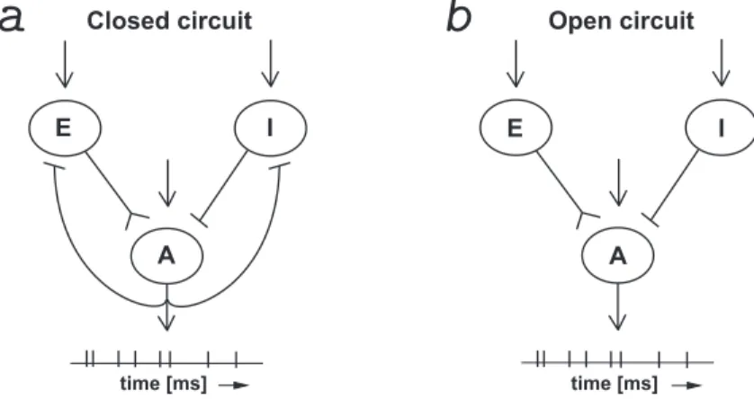
Figure 2.4. The model (2.1.14) describes a small networks of neurons with a reference unit A that receives a pool of excitatory inputs from unit E and inhibitory inputs from unit I. (a) The circuit is closed, characterized by a feedback of A on E and I that provokes a reset of the diffusion process and of the two jump process after each spike of unit A. (b) The circuit is open, with no reset of the two jump processes.

Figure 2.4 illustrates the model assuming the strong inputs project on a reference unit A from pools of excitatory E and inhibitory I units. Notice that in model (2.1.14) the process VOU J _{is reset to its initial value V}

rest after each crossing of the threshold S. It means that

also the processes N_t+ and N_t− are reset to their initial values N₀+ and N₀− after each FET. Such hypothesis is very helpful from a mathematical point of view because the sequence of FET generated by process VOU J is a renewal process, but it implies that neuron A has an inhibitory feedback on units E and I and makes the circuit closed (cf. Fig. 2.4a). The removal of the inhibitory feedback from unit A to units E and I implies that after each crossing of the threshold, processes N+ and N− are not reset to their initial values and only the diffusion process (2.1.11) is reset (cf. Fig. 2.4b). Under such assumptions the modelled

circuit can be considered an open circuit, but for a mathematical treatment of the serie of the FETs generated by the process VOU J _{it is necessary to remember that it is no more a}

renewal process.

To conclude we would like to remark that we are interested in the impact of strong postsynaptic potentials on the generation of action potentials. That is to say that we believe that there exists biological evidence of different synaptic weights and we would like to study how the sequence of action potentials elicited by the cell is affected by that. As long as the biological mechanism that leads to the generation of such strength, we consider the debate open.