Journal Pre-proof
Inclusion of water temperature in a fuzzy logic Atlantic salmon (Salmo salar) parr habitat model
J. Beaupré, J. Boudreault, N.E. Bergeron, A. St-Hilaire PII: S0306-4565(19)30401-2
DOI: https://doi.org/10.1016/j.jtherbio.2019.102471
Reference: TB 102471
To appear in: Journal of Thermal Biology
Received Date: 25 July 2019 Revised Date: 6 November 2019 Accepted Date: 24 November 2019
Please cite this article as: Beaupré, J., Boudreault, J., Bergeron, N.E., St-Hilaire, A., Inclusion of water temperature in a fuzzy logic Atlantic salmon (Salmo salar) parr habitat model, Journal of Thermal Biology (2019), doi: https://doi.org/10.1016/j.jtherbio.2019.102471.
This is a PDF file of an article that has undergone enhancements after acceptance, such as the addition of a cover page and metadata, and formatting for readability, but it is not yet the definitive version of record. This version will undergo additional copyediting, typesetting and review before it is published in its final form, but we are providing this version to give early visibility of the article. Please note that, during the production process, errors may be discovered which could affect the content, and all legal disclaimers that apply to the journal pertain.
Inclusion of water temperature in a fuzzy logic Atlantic salmon
1
(Salmo salar) parr habitat model
2
J. Beaupré1, J. Boudreault1, N. E. Bergeron1and A. St-Hilaire1, 2,* 3
4
5
1
Institut National de la recherche scientifique – Centre Eau Terre Environnement, Québec, 6
Canada 7
2
Canadian River Institute, University of New Brunswick, Fredericton, NB 8 9 10 *Corresponding author 11 Email: andre.st-hilaire@ete.inrs.ca 12
National Institute of Scientific Research 13
490 De la Couronne Street, Quebec city, QC G1K 9A9 14 Desk 2411 15 Tel: +1 418 952 5710 16 17 18
Submitted to the Journal of Thermal Biology 19
25 July 2019 20
Declarations of interest: none
21Abstract
22As water temperature is projected to increase in the next decades and its rise is clearly identified 23
as a threat for cold water fish species, it is necessary to adapt and optimize the tools allowing to 24
assess the quantity and quality of habitats with the inclusion of temperature. In this paper, a fuzzy 25
logic habitat model was improved by adding water temperature as a key determinant of juvenile 26
Atlantic salmon parr habitat quality. First, salmon experts were consulted to gather their 27
knowledge of salmon parr habitat, then the model was validated with juvenile salmon 28
electrofishing data collected on the Sainte-Marguerite, Matapedia and Petite-Cascapedia rivers 29
(Québec, Canada). The model indicates that when thermal contrasts exist at a site, cooler 30
temperature offered better quality of habitat. Our field data show that when offered the choice, 31
salmon parr significantly preferred to avoid both cold areas (<15 °C) and warm areas (> 20.5 °C). 32
Because such thermal contrasts were not consistently present among the sites sampled, the model 33
was only validated for less than 60% of the sites. The results nevertheless indicate a significant 34
correlation between median Habitat Quality Index and parr density for the Sainte-Marguerite 35
River (R2 = 0.38). A less important, albeit significant (F-test; p=0.036) relationship was observed 36
for the Petite-Cascapedia river (R2 = 0.14). In all instances, the four-variable (depth, velocity, 37
substrate size and temperature) model provided a better explanation of parr density than a similar 38
model excluding water temperature. 39
40
Keywords: Fuzzy logic, Habitat quality model, Atlantic salmon, parr, water temperature 41
42
44
1. INTRODUCTION
45
Anticipated water temperature increase in rivers linked to climatic and anthropic changes is a 46
threat to aquatic ecosystems (Isaak et al., 2018). In the recent past summers, water temperature in 47
many Eastern Canadian rivers exceeded critical thermal thresholds for many cold water fish 48
species, such as Atlantic salmon (Salmo salar) (i.e. >27.8°C; Gendron, 2013; Jeong et al., 2013). 49
Even if Atlantic salmon is commonly recognized as a relatively thermally tolerant species 50
(Garside, 1973; Jonsson et al., 2009), it is known that juvenile salmon parr become thermally 51
stressed when water temperature exceeds 23°C (Breau et al., 2011; Elliott, 1991). A continuous 52
exposure to extreme temperatures can cause massive mortalities or alter considerably the health 53
of ectotherm fishes (Garside, 1973; McCullough, 1999). Despite the relative paucity of river 54
thermal information available for North America, predictions suggest a general increase of river 55
temperature, which depends in part on latitudinal position (Morrill et al., 2005; van Vliet et al., 56
2013). 57
58
In this context, habitat models are key tools to optimize management and conservation programs. 59
In habitat modelling, classical approaches determine the quantity and quality of area potentially 60
useful for a species’ life stage or guild based either on expert knowledge or on observed habitat 61
use and physical data (Yi et al., 2017). Classical variables used in habitat model for juvenile 62
Atlantic salmon include flow velocity, water depth and substrate size (Table 1). When the model 63
is based on habitat use solely (i.e. not taking into account habitat availability), univariate Habitat 64
Suitability Indices (HSI) are defined from field measurements of presence-absence or 65
abundance/density of fish in sampling parcels. A composite HSI is calculated by combining the 66
univariate HSIs, using different methods (additive function, arithmetic mean, lowest HSI, etc.). 67
The most commonly used method thus far has been the geometric mean. A HSI of 0 describes a 68
poor habitat, while a HSI of 1 describes an optimal habitat. Multiplying the composite HSI by the 69
surface area on which it applies provides a Weighted Usable Area (WUA). This approach is often 70
used in combination with hydraulic models to provide estimates of usable areas at difference 71
river discharges (e.g. Instream Flow Incremental Methodology Bovee et al., 1998; DeGraaf et al., 72
1986; Morantz et al., 1987). 73
Combining univariate HSIs usually rely on two assumptions. First, that habitat variables are 74
independent, and second, that they exert an equal influence on habitat selection (Ahmadi‐ 75
Nedushan et al., 2008). However, those assumptions cannot be validated in most cases, as some 76
habitat variables (e.g. depth and velocity) are clearly interdependent, and some variables are more 77
important than others in the habitat selection decision. Furthermore, classical methods based on 78
field data typically require large amounts of data that are costly to acquire. They are also 79
generally obtained from a relatively small area (e.g. a single river or catchment), which makes the 80
model poorly transferable to rivers other than the one which served for calibration (Guay et al., 81
2003; Millidine et al., 2016). 82
83
To overcome these gaps, Ahmadi‐Nedushan et al. (2008) and Mocq et al. (2013) worked with 84
fuzzy systems inspired by the work of Jorde et al. (2001) who developed the Computer Aided 85
Simulation Model for Instream Flow Requirements (CASIMIR) habitat model. Those authors 86
developed salmonids fuzzy habitat models considering the classical habitat variables of water 87
depth, flow velocity and substrate size. Ahmadi‐Nedushan et al. (2008) tested the models for two 88
Atlantic salmon life stages - spawning adults and parr - and conducted a sensitivity analysis of 89
the fuzzy rules of the system based on six expert opinions. Their suggestion was to further 90
validate the model, increase the number of experts and add other habitat variables. Mocq et al. 91
(2013) improved the model by adding a life stage (young of the year) and a considerable amount 92
of experts (30 experts in total) with European and North American experience. The authors 93
partially validated their model and compared the output to a classical habitat model (Ayllón et al., 94
2012; Bourgeois et al., 1996; Gibbins and Acornley, 2000) based on Weighted Usable Areas. 95
Both models were used to assess the variation of WUA as a function of discharge and uncertainty 96
around the relations were estimated using a bootstrap method. The results indicated that relations 97
of WUA as a function of discharge were similar on both instances, even though the fuzzy model 98
was based on expert knowledge only. Mocq et al. (2015) also showed that the geographical 99
origin of the experts influenced the uncertainty associated with the delimitation of the categories 100
and they hypothesized that experts from different countries were mostly drawing their knowledge 101
from their experience from local rivers. The fuzzy logic approach also offers other advantages: 102
1) it helps describe imprecise processes through qualitative knowledge and human interpretation, 103
2) it is unimpaired by dependence between variables, and 3) it allows the easy addition of new 104
predictors or expert knowledge to the model. 105
106
Beyond the shortcomings of classical habitat models that could be addressed by fuzzy logic, there 107
are other deficiencies in current Atlantic salmon habitat models. One such deficiency is that 108
models generally neglect water temperature despite its importance for the physiology and 109
phenology of the salmon. Indeed, water temperature has rarely been included in habitat models 110
of this species (but see Stanley et al., 1995) and when it was included, it was through 111
approximation from air temperature (Caron et al., 1999). Although this deficiency was probably 112
due in the past to the lack of suitable water temperature data, there are now monitoring networks 113
of river temperature existing in the Pacific Northwest and in Eastern Canada (RivTemp, 114
www.rivtemp.ca; Boyer et al., 2016), which offer the opportunity to improve salmon habitat 115
models by adding water temperature. 116
117
The aim of this paper is to improve Atlantic salmon parr habitat modelling in Eastern Canada 118
using a fuzzy logic approach. First, a multi-expert model that includes water temperature is 119
developed to infer juvenile salmon parr habitat quality. The model is then partially validated by 120
comparing values of habitat suitability obtained from the model with parr density data collected 121
in thermally contrasted river reaches. 122 123
2. METHODOLOGY
1242.1 Multi-experts model
1252.1.1 Fuzzy sets and rules
126In the context of juvenile salmon habitat modelling, fuzzy logic is used to codify 127
experts' knowledge regarding the role of flow velocity, water depth, substrate size and water 128
temperature salmon parr habitat quality. 129
130
The first step in designing a fuzzy model is called “fuzzification”. The purpose of this step is to 131
divide each input variable into categories. In this case, input and output variables were classified 132
as “low”, “medium” or “high”. As an example, flow velocity was categorized as either “slow”, 133
“medium” or “fast”. The fuzzyfication was completed by interviewing experts on the selected 134
habitat variables and their impact on the suitability of parr habitat. The experts were ask to divide 135
the range of possible values of each variable into three categories using more or less precise 136
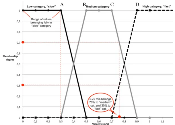
ranges of values. The separation of variables into categories is done by assigning a membership 137
degree to the values, thereby creating a membership function (Figure 1). A habitat variable (e.g. 138
velocity) value with a membership degree of 0 means that it does not belong to the category. 139
Conversely, a membership degree of 1 means that this habitat variable value belongs totally to 140
the category. For each variable, the experts targeted ranges of values for which they were certain 141
of full membership (i.e., membership degree =1) in the categories. 142
143
As working with nominal categories leads to uncertainties, the experts were given the opportunity 144
to leave a range of values that can belong to two categories, thereby representing the uncertainty 145
(or fuzziness) of the expert on the definition of boundaries between categories (e.g. for velocity, 146
0.3-0.5 m/s; 0.7-0.9 m/s; Figure 1). The uncertain intervals are called the “fuzzy zones”. It is 147
possible to model a value in a fuzzy zone by attributing it proportionally to two categories at the 148
same time. To help the expert delineate the categories, we asked them to think about parr habitat 149
in a context of survival. We did not predetermine upper boundary values for the variables. The 150
experts had to fix them themselves according to their experience. 151
152
Once the categories were delimited, the experts had to qualify the habitat resulting from the 153
combination of each category of variables. The fuzzy rules are all constructed using the following 154
format: IF the substrate size is large, AND IF velocity is medium AND IF depth is low AND 155
temperature is warm THEN habitat suitability is... either "poor", "medium" or "high" according 156
to experts. Considering three categories for each of the four variables, there are a total of 81 157
combinations and their consequences (habitat suitability) are defined based on the experience of 158
the respondent. Some habitat variables combinations are not found or are very rare in nature and 159
therefore, are rarely used in the model. For example, if an expert determined that a fast velocity is 160
greater than 2 m/s and a small substrate is less than 2mm. All the rules involving a fast velocity 161
and a small substrate would be unrealistic because in rivers, the water flowing at such high 162
velocity would most likely flush out such fine substrate. 163
164
2.1.2 Experts selection
165From April to October 2017, we interviewed experts with a concrete knowledge of Atlantic 166
salmon parr habitat in order to gather and codify this knowledge (Mocq et al., 2015). We 167
gathered the opinions of 22 experts through meetings of which 18 answered the questions on 168
their own. Two teams of two were also counted as one expert each. Among the participants, 17 169
work in the public sector, while five are in the private sector. Public organizations include 170
teaching and research institutions (8), government departments (5) and non-profit organizations 171
(5). There were eight technicians, three professors, eleven managers and three graduate students. 172
Some of them occupied more than one position. Our primary criterion for selecting an expert was 173
that the person had at least one year of hands-on experience with Atlantic salmon parr in Eastern 174
Canada to optimize the model for this region, as the origin of the expert has been shown to 175
influence the model outcome (Mocq et al., 2015). The geographic origin of the expert's 176
experience has been separated into seven different groups: Saguenay (15 experts; Qc), North 177
Shore (10 experts; Qc), Ungava (3 experts; Qc) and Québec City area (1 expert; Qc) which are 178
located on the north shore of the St. Lawrence River. Lower-St.Lawrence (6 experts; Qc), 179
Gaspésie (10 experts; Qc) and New-Brunswick (3 experts; NB) are located south of the St. 180
Lawrence River. Their knowledge about habitat preferences could come either from literature or 181
field experience. We did not measure their level of expertise, however experts were asked to rate 182
their level of confidence in their response from 1 (low confidence) to 10 (high confidence). We 183
also contacted some of the experts who had already done a similar exercise with Mocq et al. 184 (2013). 185 186
2.2 Field sampling
1872.2.1 Sites selection and description
188The second specific objective of the project was to validate whether the experts’ opinion was 189
consistent with what we could observe in the river. Site selection was based on three main 190
criteria. The first was presence of parr in the site area. The second criterion refers to the initial 191
hypothesis of the study, i.e. that water temperature influences the quality of parr habitat as 192
defined by the expert and that it influences habitat selection. Thus, we looked for sites where 193
there was a potential thermal contrast such as a confluence of a river with a colder or warmer 194
tributary. Since the hypothesis guiding the study was temperature-related, we defined the two 195
compared areas as the “warm area” and the “cold area”. To better understand the sampling 196
protocol, Figure 2 illustrates the definition of what is considered in this project as a site, an area 197
(cold or warm) and a patch. The last criterion to choose the site was that similar habitats (depth, 198
velocity and substrate size) exist in the warm and the cold areas. Comparing similar habitat types 199
in both areas is an attempt to isolate the effect of water temperature.
200 201
The warm and the cold areas had to be more than two meters wide and no less than 40 m2 each. 202
The sampled area could be located directly in the tributary, in the tributary plume downstream of 203
the confluence, upstream or downstream in the main channel, as long as the temperature was 204
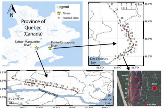
different and the other variables were comparable. According to those criteria, four sites were 205
selected. The A and B sites are in the Sainte-Marguerite River (SMA). This 100 km long river is 206
in a mainly forested area between Chicoutimi and Sacré-Coeur on the Quebec North shore, 207
Canada. The salmon population for this river was about 360 spawning adults in 2016 (MFFP, 208
2017) and the regional average summer air temperature for the last ten years is about 20.8 °C. 209
The C and D sites are in the Matapedia River catchment on the Quebec South shore, Canada. 210
Mean summer air temperature is about 21.6 °C. Spawning adult population on this river was 211
about 1940 in 2016 (MFFP, 2017). Figure 3 gives more details about the geographic position of 212
the sites. In total 12 surveys were completed, which consist of electrofishing and habitat 213 characterization. 214 215
2.2.2 Electrofishing protocol
216A field campaign was undertaken from July 20th to September 26th 2017. We sampled five times 217
site A, three times site B, three times site C and one time site D to compare parr densities in two 218
thermally contrasted areas (see Figure 3). Only a partial validation was performed since, as 219
previously explained, it is not the full suite of 81 fuzzy rules that were found to apply when using 220
variable values measured in the field during the sampling campaign. Furthermore, the 221
electrofishing method restricted the sampling areas to relatively shallow reaches with relatively 222
slow flowing water. We could not fish in an area deeper than hip height or when the water 223
velocity was greater than 1.5 m/s with water depth higher than the knees. 224
225
When arriving at a fishing site, the area was scanned using the Seek Thermal Compact XR device 226
to visualize water temperature spatial variability. Figure 4 shows a typical site picture taken with 227
the thermal camera. This infrared camera picture was assessed against spot measurements of 228
temperature using a digital thermometer. Depending on the availability of contrasted habitat 229
observed by thermal camera, warm and cold areas were delimited to form fishing zones, each 230
with an area between 50 and 150 m2 (Figure 2). In a designated site, we tried to compare areas 231
with roughly the same surface area. Habitat use was evaluate by electrofishing in groups of three 232
people. The team included one person handling the electrofisher (Smith-Root LR-42 model) 233
accompanied with two catchers holding a net. The electrofisher parameters (voltage, frequency, 234
duty cycle) were programmed in “Direct Current” and according to water conductivity with the 235
automatic “Quick set-up” option in the menu. The voltage was adjusted in increments of 20 V 236
until the optimum fish response was achieved, that is, galvanotaxi (e.g. 237
involuntary swimming towards the anode) followed by a vigorous recovery in the following 20 238
seconds. The electrofisher holder was placed upstream and perpendicular to the catchers to 239
perform a large sweeping gesture with the anode (“M” shaped motion) in front of them, shocking 240
an area of approximately 0.80 m2. The electrofishing was repeated and carried out to cover the 241
entire delimited area. 242
243
When a parr was caught, its location was identified with a tag, the temperature was measured and 244
the fish was placed in a container. The captured specimens were all weighed and measured. If 245
two individuals were captured in the same 0.5 m radius patch (Keeley et al., 1995; Lindeman et 246
al., 2015), they were associated with the same habitat measurements. Once the measurements 247
were made, fish were returned to the river, downstream of the sampling area. The electrofishing 248
was made from downstream to upstream while taking care never to trample the patches before 249
fishing. The same exercise was performed in the cold and the warm area. We noted the total 250
fishing time in each thermally contrasted area to ensure a constant fishing effort and the number 251
of parr caught in each area have been used to calculate a density over a surface of 100 m2. 252
253
2.2.3 Habitat
254In the sampling areas, habitat variables were also surveyed in at least ten patches where no fish 255
was caught or observed. While performing the electrofishing, patches were selected in a stratified 256
random manner, so that the range of available velocities, depth and substrate were covered in the 257
samples. The selected patches for characterization were also identified with tags. Temperature 258
was measured instantly because it is a variable that can change over the fishing period. Once 259
electrofishing was completed in the areas, the other habitat variables were measured at each 260
location. The diameter (B-axis) of the dominant substrate was evaluate out of the 0.79 m2 261
window around the tag. Depth and velocity at 40% of the total depth of the water column from 262
the bed (Marsh McBirney flowmeter) was taken at the focal location of the tag. Sampling tags 263
(placed for fishing and/or characterisations) were never located in the same 0.79 m2 habitat patch. 264
At every site, two temperatures sensors (Hobo Pendant Temperature/Light Data Logger) were 265
also placed, one in the main channel and one in the tributary. Water temperature ± 0.5 °C was 266
recorded every 15 minutes from July 4th to September 20th 2017 to characterize the plume at sites 267
A and B and to assess the thermal contrast between the receiving river and the tributary at sites C 268 and D. 269 270
2.3 Model application
271All field measurements were used as inputs in the fuzzy logic model to calculate Habitat 272
Suitability Indices (HSI) using the Fuzzy logic toolbox in Matlab R2016b software. The toolbox 273
is used for the construction of fuzzy sets using linear functions defined by the experts. The rules 274
defining how each combination of habitat variables lead to different HIS categories are also 275
entered. Like Mocq et al. (2013) and Ahmadi‐Nedushan et al. (2008), the Mamdani inference 276
was used to calculate HSI of patches sampled in the summer of 2017. This implies that when two 277
fuzzy sets are combined in a rule, with specific membership function values, the minimum is 278
used to quantify the membership function value of the HSI. When more than one rule is needed 279
to describe the combination of habitat variables, the resulting fuzzy set is a sum of the HSI 280
membership functions. 281
282
The two main steps in the fuzzy inference used to calculate HSI are called the implication and the 283
defuzzification. This latter step allows to convert a fuzzy HSI set to a real HSI value. Those 284
operations were completed for all sampled habitat patches, considering individual expert fuzzy 285
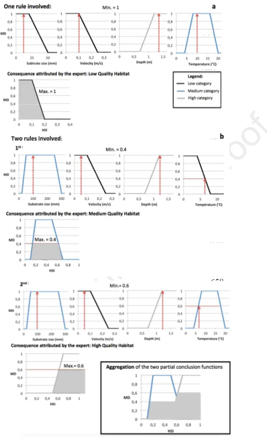
sets and rules separately. When the values of all the habitat variables in the patch have a full 286
membership to their respective category (membership degree of 1), a single fuzzy rule is 287
involved. In this case, the conclusion function is defined by the full range of the consequence of 288
the rule determined by the expert (low, medium or high habitat quality). As illustrated in 289
Figure 5, considering a substrate of 12 mm, a velocity of 0.1 m/s, depth: 1.4 m and a temperature 290
of 10°C, an expert model would considerer that his patch has a small substrate, low velocity, high 291
depth, medium temperature and the consequence of this combination is low HSI. Since all the 292
variables in the parcel have a membership degree (MD) of 1, the minimum of the conclusion 293
function (implication) is also 1 or 100%. The numerical HSI of the patch will be determined by 294
defuzzifying using the center of gravity of the area under the curve of the conclusion function. 295
296
Sometimes, many rules are necessary to describe a patch. Depending on the expert, the number of 297
fuzzy rules applying to a habitat patch can vary between one to a maximum of 16. For instance, if 298
the values of three variables (out of four) in the patch are in a fuzzy zone (i.e. having membership 299
in two categories), eight rules will be needed to describe the patch. As seen on Figure 5, when 300
one value is in the fuzzy zone, two rules are necessary to describe the patch. Supposing a patch 301
with a median substrate diameter of 100 mm, a velocity of 0.5 m/s, a depth of 1.2 m and a 302
temperature of 6 °C (in the fuzzy zone). According to this expert this patch has a small substrate, 303
low velocity, high depth. Temperature belongs partly to the medium and partly to the high 304
categories and the consequence of this combination is an aggregation of medium and high habitat 305
quality. As the minimum membership degree (MD) among the variables for the first rule is 0.4, 306
the membership of the partial conclusion function is also 0.4 and it is 0.6 for the second rule. 307
Making an aggregation, by combining the fuzzy sets representing the conclusion functions of 308
each rule, provides the total conclusion set. The center of gravity of the area under the curve of 309
this resulting aggregated fuzzy set becomes the numerical value of the HSI. 310
311
2.4 Model validation
3122.4.1 Validation in a thermal contrast 313
The partial validation of the model was completed for every electrofishing and habitat survey 314
(one day, one site), considering all experts’ fuzzy models separately. A HSI was calculated for 315
each sampled habitat patch, in presence and in absence of parr. Then, a non-parametric Kruskal-316
Wallis test was used to verify the null hypothesis that the median HSI of the warm and cold areas 317
of a fishing survey were equal with a confidence level α=0.05. To facilitate the description of the 318
results, we identified so-called “significant experts” when the experts’ model rejected the null 319
hypothesis for an electrofishing survey, i.e. the model showed a significant difference in HSI 320
values between thermally contrasted habitats. The global model was considered validated when 321
the majority of the significant experts express a higher HSI in the area where higher parr density 322
was measured. 323
324
2.4.2 Validation of observed densities 325
326
A second partial model validation was conducted using a different data set from field surveys 327
undertaken during summer 2017 between July 27th and September 16th on the Sainte-Marguerite 328
(previously described in Section 2.2.1) and the Petite-Cascapedia rivers located in the Gaspésie 329
region (Eastern Québec). See Figure 6 for rivers location. On these rivers, various sites were 330
surveyed to cover a wide heterogeneity of salmon habitat. In total, 30 sites were surveyed on the 331
Petite-Cascapedia River whereas 27 sites were surveyed on the Sainte-Marguerite River. These 332
sites were at least separated by 500 m along watercourse to ensure independence between sites. 333
At each site, 30 equally spaced 4 m2 patches along 5 transects (6 patches per transect) were 334
electrofished and physically characterized as illustrated on Figure 6. The same physical habitat 335
variables were measured at each of those patches (depth, velocity, substrate size and water 336
temperature). The only difference is that the velocity and temperature were measured using an 337
acoustic velocity meter (Sontek Flow Tracker 2) on the Petite-Cascapedia River. After all 338
measurements were completed in all patches, the mean value of these measurements was used as 339
an input for the expert’s models to obtain a HSI value for each of the sites. Finally, electrofishing 340
was conducted using also the Smith-Root LR24 Electrofisher at each of these 30 patches. The 341
parr density for a site was then obtained by summing the individual parr densities at each patch 342
within the site. Hence, the relation between the HSI given by the experts and the relative parr 343
density at each site can be investigated as another validation of the developed expert model. 344
3. RESULTS
346
3.1 Experts based model
347All 20 experts had to design fuzzy sets for each of the four input variables (temperature, velocity, 348
depth and substrate) with three categories (low, medium, high). Table 2 shows the medians and 349
ranges (maximum and minimum) of selected limits for fuzzy sets defining the categories of 350
habitat variables. It can be seen that typically the variability (median/range) is between 0.2 and 351
2 %. For instance, experts defined roughly the “low” category for temperatures between 0 and 8 352
°C, “medium” category between 12 and 18 °C and “high” category over 22 °C. 353
354
The 20 experts had to assign a consequent Habitat Suitability (poor, medium or high) for each 355
combination of velocity, depth, substrate and temperature categories. Like Mocq et al. (2013), we 356
identified the most frequently selected consequent HSI category as the “consensus” response and 357
we calculated how many experts were part of this consensus. Considering the 81 rules, experts 358
have a mean consensus of 63.7 %. In others words, about 13 experts out of 20 generally agree on 359
rules consequence. Experts attributed a poor habitat for 64% of the rules, with a consensus of 360
68%. For half of those rules, there is about 11% of the experts that conclude, conversely, that 361
these same rules lead to a high habitat quality. About 25 % of the rules have “medium” HSI as 362
consequence, with a consensus of 53%. Only 9% of the rules have been associated with a “high” 363
HSI and about 56% of experts were part of this consensus. For 71 % of the rules with a high HSI 364
consequence, a minority (2.8 %) of the experts concluded the opposite, i.e. that habitat was of 365
poor quality. Two rules have no consensus, i.e. different consequent categories were selected by 366
an equal number of experts. 367
368
3.2 Habitat characterization
369During the summer, water temperature was measured every 15 minutes for July 7th to September 370
20th. The average summer water temperature in the main channel and in the tributary as well as 371
the maximum temperature reached for study sites are compiled in Table 3. For all surveys, 372
physical habitat variables measurements were taken. Median values measured for the velocity 373
ranged from 0.11 to 0.76 m/s, depths ranged from 0.11 to 0.38 m and substrate sizes ranged from 374
85 to 190 mm. Median temperatures ranged from 13.1 °C to 19.5 °C in the cold areas and from 375
16.1 °C to 21.8 °C in the warm areas. The thermal contrasts (median temperature differences) 376
between cold and warm areas varied from 1.4 °C to 6.0 °C. For all electrofishing surveys 377
completed, this thermal difference was statistically significant (Kruskal-Wallis; p < 0.05). 378
Despite efforts to sample areas with similar values for habitat variables other than temperature, 379
for four electrofishing surveys, there were two significantly different habitat variables including 380
water temperature and three surveys had three significantly different variables between cold and 381
warm areas, when the Kruskall-Wallis test was applied. Table 4 gives more details about the 382
median values of the variables sampled for each electrofishing survey.. 383
We characterized a total of 451 patches. From these measurements, a HSI value was calculated 384
for each of the 20 experts. The analysis of the 451 patches also generated 21 031 applications of 385
66 different rules. The other 15 rules were never used. The most frequently used rule (3 798 386
times) is when the values of the four variables belong the medium category, represents 18% of 387
uses and 80% of experts agree on the consequent HSI for this rule (high HSI). The seven most 388
frequently used rules are shown in Table 5. They represent 63% of rule applications, with a mean 389
expert consensus of 60%. 390
As already stated, HSI for each of the 20 experts were calculated for each sampled habitat patch. 391
The mean standard deviation for HSI was 0.18 (HSI varies between 0 and 1). Only expert models 392
that expressed a significant difference between median habitat quality in the colder and the 393
warmer area were considered to partially validate the model. As shown in Table 6, four experts 394
expressed significant differences for more than 90% of the fishing surveys, two experts never 395
expressed significant differences and two other expressed differences for less than 10 % of 396
fishing surveys. For 50% of the surveys, experts that concluded to significant differences were 397
unanimous to determine that the colder area had the highest habitat quality. For 17% of the 398
surveys, opinions were more split. Respectively for site A day 269 and site B day 201 (Table 5), 399
56% and 57% of the significant experts agreed that the cold area was of better quality compared 400
to 44% and 43% who said the opposite. For the other surveys, over 70% of the experts agreed on 401
the model conclusion. 402
403
3.3 Electrofishing
404For our analysis, we considered only the specimens with fork length >55 mm as parr. A total of 405
226 parr (1+ and 2+), in 201 different patches were captured or clearly observed during the 406
summer. For all the electrofishing surveys, we standardized the number of fish that we caught in 407
each area (colder vs warmer) by prorating densities for an area of 100 m2. As seen in Table 4, 408
among all the electrofishing surveys, the highest density of fish was found in median temperature 409
ranges of 15.2 to 20.2 °C, which is in agreement with the known temperature optimum for parr 410
feeding (15 to 19 °C according to the literature; DeCola, 1970; Elliott, 1991; Elson, 1969; Stanley 411
et al., 1983). We did not find any fish in the warmest area (21.8°C). Moreover, when the warm 412
areas exceeded 20.9 °C, 42% more fish were caught in the colder area. We also saw that when 413
the colder area offers temperatures lower than the feeding optimum range (<15.0 °C), parr were 414
mostly found (48% more) in the warm area. 415
416
3.4 Model application and validation
4173.4.1 Validation in a thermal contrast 418
419
As indicated in Table 4, the model was partially validated seven times and was shown to be 420
inconclusive five times. As already explained, validation was conclusive when the highest fish 421
density was found in the area with the highest modelled HSI values for a majority of experts. 422
Every time the model was not validated, most of experts predicted a better quality of habitat in 423
the cooler area while the highest parr density was in the warmer area. For site A, the model was 424
validated three times out of five surveys. When the model was not validated for this site (day 214 425
and 229; table 4), the temperatures of the cold area were respectively 14.2 and 13.1 °C. For 426
day 214, we note that the velocity and the substrate size were also significantly different between 427
the two areas (lower velocity and larger substrate in the warm area). For site B, the model was 428
always validated. At that site, temperature values were always in a range that is adequate for parr 429
(15.2-20.9 °C). For day 201, depth was significantly higher in the warm area (0.21 vs 0.33 m) 430
than in the colder area and for day 209, the substrate was significantly larger in the colder area 431
(100 vs 140 mm) than in the warmer area. At site C, the model was invalidated for the first two 432
electrofishing surveys. In the first case, the temperature of the cold area was 13.9 °C while 433
temperature in the warm area was 19.2 °C. Also, the velocity and the substrate size were 434
significantly higher in the cold area than in the warm area. In the second case, the temperature of 435
the cold area was 16.1 °C while the temperature of the warm area was only 19.3 °C. The velocity 436
was also significantly faster in the cold area. The model was validated for the third electrofishing 437
survey at this site while the temperature in the warm area was 21.1 °C and 16.2 °C in the cold 438
area. The depth was also significantly greater in the warm area (0.11 vs 0.17 m) and the substrate 439
was larger in the cold area (90 vs 105 mm). Finally, for site D, the model has not been validated 440
for the only electrofishing survey that was completed at that site. The temperatures in the warm 441
and cold areas were respectively 18.3 °C and 16.5 °C. 442
3.4.2 Validation of observed densities 443
444
Validation of the model with the additional dataset collected on Sainte-Marguerite and Petite-445
Cascapedia River is shown in Figure 7. This figure illustrates the link between the logarithmic 446
transformation of parr density (1+ and 2+) at each site and predicted HSI from the model 447
considering only depth, velocity and substrate size (a) vs our expert’s model including the same 448
three variable and water temperature (b). Our model explains respectively 37% and 15 % of the 449
parr density for Sainte-Marguerite and Petite-Cascapedia rivers while the model without water 450
temperature explains respectively 18% and 1%. Based on a F-test comparing the model that
451
includes HSI to explain log density to a simpler model that includes only an intercept, the p-value of
452
0.036 means that the model that includes HSI is significantly different than an intercept-only model.
4. DISCUSSION
454
The main objective of this project was to include water temperature in an expert based model to 455
better quantify and qualify habitat preferences for Atlantic salmon parr. This main objective was 456
achieved by completing two steps. The first one was to codify the knowledge of selected experts 457
on four habitat variables: water temperature, depth, velocity and substrate size. These experts also 458
had to qualify the Habitat Suitability Index resulting from the different combinations of these 459
variables. The second step was to perform a partial validation of the model by putting field data 460
into the model in order to obtain a numerical HSI, and compare it against parr density with and 461
without a thermal contrast at different sites. This work therefore presents an improvement from 462
the models developed by Ahmadi‐Nedushan et al. (2008) and Mocq et al. (2013). 463
464
We selected 20 professionals with an Eastern Canadian experience to optimise the model for this 465
region. The model has been validated for 58 % of the surveys. Considering that it is the first 466
fuzzy model that includes water temperature for Atlantic salmon parr, and considering that 467
sampling was completed in a summer with relatively low temperature contrasts (i.e. no heat 468
waves or sustained warm periods) this result is promising and constitutes an important 469
advancement. 470
471
The first validation method aimed to compare habitat quality between cold and warm areas. 472
When the model was not validated, it predicted that higher quality habitat would be in a cold 473
area, whereas parr were mostly in warm areas. We suspect that the main cause explaining why 474
42% of the electrofishing surveys did not agree with the model is that the summer 2017 in 475
Quebec was not particularly warm and hence, cold water temperature refuges in the sampled 476
rivers were often not necessary for parr. The temperature sensors placed at the sites under study 477
revealed that the hottest temperature of the water during the summer period, all sites combined, 478
was 25.8°C which is not close to the upper incipient lethal temperature for parr (27.8 °C; death of 479
50% of fish after 7 days). When this temperature was reached, it generally lasted for less than two 480
hours. For sites A, B and C there was respectively 19, 7 and 18 days where temperature exceeded 481
22 °C. This temperature represents the upper critical range where normal metabolic functions 482
cease, but parr can still survive for a long period of time at that temperature (Jonsson and 483
Jonsson, 2009). However, 22 °C exceedances never persisted for more than 12 hours. At night, 484
the temperature generally decreased below 20 °C. This might give a respite to fish by recreating 485
the effect of a thermal refuge. Nonetheless, at site D, there were 31 days where temperature 486
exceeded 23 °C and rarely cooled down below 20 °C. There was a particular warm period 487
between day 195 and day 207 (from July 17 to July 23) where the average daily water 488
temperature remained above 22 °C. The maximum temperature reached during this period was 489
25.8 °C while the minimum never went below 20.6 °C, which is considerably high for a 490
prolonged period. Even if Site D was the warmest, our only electrofishing survey at this site was 491
completed during a cooler period and we suspect that is the reason why the model was not 492
validated for this survey. Furthermore, among all the surveys, it was common to compare two 493
areas whose average temperatures were both in the tolerable, almost optimal range for parr. Such 494
ranges generally do not trigger movement to cold refugia (Breau et al., 2011). 495
496
We also attempted to test and compare the proposed model on a different, larger dataset, which is 497
an approach suggested by many authors (Fukuda, 2009; Kampichler et al., 2000; Mouton et al., 498
2008). We can see on Figure 7 that in both cases, our four-variable model explains better parr 499
densities then the three-variable model, and this, for every site. This suggests that adding a 500
variable such as water temperature improves the predictability of the model. The correlation 501
between the median HSI and the density of parr is weaker for Petite-Cascapedia (R2 = 0.15) than 502
for Sainte-Marguerite data (R2 = 0.37). This could be explained by the low heterogeneity of the 503
habitats studied on the former river. In fact, the lowest HSI model assigned in the Petite-504
Cascapedia River was 0.4, which is generally considered an average value, according to most 505
experts. Thus, the patches sampled were all of considerable interest for parr and relatively 506
similar. It goes without saying that all the parcels cannot be occupied, thus leaving several 507
interesting habitat patches vacant. Although the concept of transferability is not accepted by all 508
(Groshens and Orth, 1993; Leftwich et al., 1997; Strakosh et al., 2003), the correlations revealed 509
by these linear regressions allow us to be enthusiastic about the possibility of transferring this 510
model to several rivers. Although some authors have tested the transferability of regional models, 511
the correlation that we obtained on the Sainte-Marguerite River has not, to our knowledge, been 512
previously equaled (e.g. R2 = 0.02 to 0.31; Guay et al., 2003, Hedger et al., 2004). The fact that 513
the correlation is considerably higher for the Sainte-Marguerite River raises new questions about 514
the possible bias of the experts, some of whom may have never seen rivers such as the Petite-515
Cascapédia. In fact, it is possible to note that the expertise of our respondents comes mainly from 516
the north shore of Quebec (60%). Thus, perhaps the model could be better optimized for cooler 517
rivers considering that the specific adaptations of juveniles in the north and south may be 518
different (Glozier et al., 1997, Hedger et al., 2004). 519
520
Even if the proposed model is less parsimonious than its predecessors, it is still a simplification 521
of a complex system that influences parr habitat selection. It includes only four physical 522
variables, but excludes many important ones for habitat selection such as habitat connectivity 523
(Bardonnet et al., 2000), biomass cover and food abundance (Wilzbach, 1985), circadian and 524
seasonal cycle (Cunjak, 1996; Mäki-Petäys et al., 2004), density dependent relationship (Jonsson 525
et al., 1998; Lindeman et al., 2015), etc. As habitat selection by parr is based on many biotic and 526
abiotic factors (Armstrong et al., 2003; Klemetsen et al., 2003), it has been shown many times 527
that HSI and WUA are ambiguous concepts because it is often hard to link them to fish 528
abundance and density (Bourgeois et al., 1996; Milhous et al., 1989). Even in the case where a 529
large number of good habitat patches exist on a river, parr could actually use few of them. 530
Conversely, it is also possible to find parr in habitats of poor quality with little or no explanation 531
for their presence. 532
533
Globally, our expert models suggest that a cooler temperature would offer a better habitat quality, 534
which is probably more exact during warmer periods but less accurate when both sections offer a 535
tolerable range of temperature or a contrast that is not optimal, e.g. an area that is too cold vs a 536
tolerable warm area. We did see that when the warm area was hotter than 20.8 °C, the model is 537
always validated and parr were mostly in the cold area as predicted by the experts. This 538
systematic validation for higher temperatures suggests that the model is adequate when limiting 539
temperatures are reached (Breau et al., 2007; Elliott and Elliot, 2010; Jonsson et al., 2009). 540
541
On the other hand, even if parr can survive near 0° C and still feed at 3.8 °C (Elliott, 1991), 542
growth is largely linked to feeding (Storebakken et al., 1987) and it starts being suboptimal 543
below 15 °C (DeCola, 1970). Despite this, for some electrofishing surveys, the majority of 544
significant experts indicated that 14.2 °C, 13.1 °C and 13.9 °C would offer respectively better 545
habitat quality than 20.2 °C, 16.1 °C and 19.5 °C. Our electrofishing results suggest that this may 546
not be accurate. In that context, it would be beneficial to review with the experts, the parameters 547
assigned for the temperature categories, and the consequent HSI category (de Little et al., 2018). 548
Especially considering that a part of the model bias could come from an incomplete 549
understanding of the instructions to prepare the fuzzy model for the expert or from a 550
misinterpretation between the interlocutors. For this model, we suspect that questioning the 551
expert in a feeding context rather than in a survival context would provide a better setting when 552
discussing parr preferences. 553
554
Also, several experts verbally testified during the exercise that having four categories instead of 555
three for the output variable (habitat quality) would facilitate the attribution of consequences to 556
the rules. These categories could be poor, medium, high and very high HSI. Unlike adding a 557
category to input variables, adding an output category would not affect the number of rules to 558
answer by experts. This modification could be done during a new consultation with the experts. 559
560
As many other studies on habitat model there is still a need for further validation to prove that 561
this model could be an effective management tool (Ahmadi‐Nedushan et al., 2008; Bargain et al., 562
2018; Guay et al., 2000; Lamouroux et al., 2002; Mocq et al., 2013). Even if multiple-experts 563
based model have been identified as potentially highly exportable (Annear et al., 2002) It would 564
be important to gather data from other studies on parr from different river types and different 565
thermal regimes for further validation. Additional validation should include sites within a river 566
that are separated by a distance that is sufficient to minimize the risk of movement of individual 567
fish from the warm to the cold area during sampling. 568
Acknowledgments
570The authors would like to thank the partners and the funding organizations: Mitacs Accelerate, 571
the Atlantic Salmon Conservation Foundation as well as la Fondation Saumon for their 572
generosity. We also want to thank all the technicians, colleagues and interns who help 573
accomplish fieldwork as well as the scientific support provided by members of the research 574
groups of A. St-Hilaire and N. Bergeron. Warm thanks to all the experts who participated in 575
building the model. 576
Tables
577
Table 1: Preferred parr physical habitat variables ranges found in the literature
578 579
Depth (m) Velocity (m/s) Substrate (mm) Reference 1+ parr*
0.10-0.40 0.00-0.20 16-256 Heggenes et al., 1999 0.16-0.28 0.10-0.30 - Gibson, 1993 0.10-0.35 0.15-0.60 25-125 Scruton and Gibson,
1993 0.1-0.50 0.00-0.60 Gravel-pebbles Jonsson and
Jonsson, 2011 0.20-0.40 0.20-0.60 20-200 Finstad et al., 2011 2+ parr**
0.17-0.76 0.35-0.80 200-300 Armstrong et al., 2003 < 0.50 0.0-0.25 Small gravel and
cobble
Gibson, 1993 0.20-0.60 0.03-0.25 64-512 Heggenes et al.,
1999 0.19-0.31 0.11-0.29 Gibson, 1993 0.10-0.55 0.10-0.70 30-200 Scruton and Gibson,
1993 0.10-0.80 0.0-0.80 Gravel, pebble, cobble Jonsson and Jonsson, 2011 0.20-0.70 0.00-0.90 25-450 Finstad et al., 2011 * Second summer of growth in river
580
**Third summer of growth in river
581
Table 21: Medians and ranges (maximum and minimum) of selected limits for fuzzy sets defining the categories of habitat variables.
582 Substrate size (mm) Velocity (m/s) Depth (m) Temperature (°C) A B C D A B C D A B C D A B C D Minimum 5 10 45 64 0.05 0.2 0.45 0.55 0.02 0.15 0.35 0.4 4 8 16 19
Median 20 50 240 300 0.15 0.28 0.6 1 0.15 0.3 0.73 1 8 12 18 22
Maximum 100 200 700 1000 0.6 0.8 1.3 1.8 0.3 0.5 2 5 19 22 25 30
Where A represents the upper limit values fully belonging to the low category, B and C the limits of the values fully belonging to the medium category and D the
583
lower limit of the values fully belonging to the high category. See Figure 1
584 585
Table 3: Average summer water temperature in the main stem and in the tributary for study sites from July 4th to September 20th 2017
586 Main stem temperature Tributary temperature Maximum temperature* (°C) Site A 17.3 10.7 25.2 Site B 16.5 14.8 23.5 Site C 17.7 15.4 25.3 Site D 14.8* 20.7* 25.8
*experienced at the site
587 588 589 590 591 592
Table 4: Median values for each sampled variable and parr density (standardized on 100m2) in the different areas (warm and cold) for each electrofishing
593 survey. 594 Day of the year Depth (m) Velocity (m/s) Substrate size (mm) Temperature (°C ) Fish density Model validation
Cold Warm Cold Warm Cold Warm Cold Warm Cold Warm
A 201 0.29 0.38* 0.29 0.42 110 145 17.6 21.8* 14 0 Yes
214 0.23 0.20 0.24* 0.13 115 175* 14.2 20.2* 9 28 No 229 0.22 0.26 0.20 0.11 150 140 13.1 16.1* 7 11 No 269 0.24 0.28 0.27 0.40 85 88 17.1 20.1* 7 6 Yes B 201 0.21 0.33* 0.48 0.71 90 120 19.5 20.9* 5 3 Yes 209 0.28 0.34 0.76 0.74 140* 100 15.2 18.1* 13 1 Yes 215 0.27 0.29 0.68 0.63 120 120 17.0 19.2* 7 0 Yes C 206 0.32* 0.20 0.52* 0.42 165 190 13.9 19.5* 4 22 No 212 0.19 0.22 0.33* 0.24 110 130 16.1 19.3* 9 20 No 234 0.11 0.17* 0.26 0.36 105* 90 16.2 21.1* 16 13 Yes D 206 0.22 0.25 0.43 0.52 100 95 16.5* 18.3* 6 14 No
(*) indicates that the median was significantly higher.
595
Table 5: The most frequently used fuzzy rules
596
Rule Substrate Velocity Depth Temperature
Number of applications
41 Medium Medium Medium Medium 3798
42 Medium Medium Medium Warm 2047
29 Medium Slow Low Medium 1927
32 Medium Slow Medium Medium 1789
68 large Medium Medium Medium 1379
50 Medium Fast Medium Medium 1162
33 Medium Slow Medium Warm 1074
Table 6 : Median HSI for both warm and cold areas of each site, according to the 20 experts
597
Experts Sites
Day of
the year Sections 1 2 3 4 5 6 7 8 9 10 11 12 13 14 15 16 17 18 19 20
A
201 cold 0.57 0.68 0.59 0.64 0.33 0.54 0.64 0.65 0.53 0.77 0.56 0.53 0.81 0.86 0.48 0.72 0.70 0.37 0.52 0.43
warm 0.38 0.34 0.29 0.80 0.30 0.63 0.78 0.87 0.55 0.80 0.33 0.59 0.36 0.29 0.50 0.55 0.73 0.13 0.54 0.48
208 cold 0.60 0.64 0.69 0.56 0.31 0.54 0.51 0.57 0.38 0.49 0.67 0.51 0.61 0.88 0.50 0.60 0.62 0.47 0.29 0.20
214 cold 0.66 0.70 0.69 0.55 0.30 0.54 0.43 0.53 0.40 0.54 0.68 0.51 0.64 0.87 0.50 0.60 0.59 0.48 0.24 0.26 warm 0.38 0.62 0.46 0.52 0.30 0.53 0.44 0.49 0.18 0.46 0.33 0.50 0.42 0.87 0.50 0.61 0.59 0.12 0.17 0.17 229 cold 0.79 0.75 0.69 0.61 0.30 0.56 0.41 0.58 0.55 0.63 0.68 0.51 0.75 0.87 0.50 0.64 0.64 0.48 0.23 0.27 warm 0.77 0.62 0.69 0.53 0.35 0.56 0.35 0.57 0.54 0.41 0.68 0.52 0.54 0.87 0.50 0.67 0.69 0.47 0.15 0.17 269 cold 0.61 0.63 0.50 0.49 0.32 0.54 0.47 0.60 0.52 0.68 0.59 0.51 0.73 0.86 0.50 0.68 0.64 0.38 0.37 0.43 warm 0.38 0.66 0.40 0.80 0.31 0.53 0.70 0.78 0.52 0.80 0.33 0.63 0.52 0.86 0.31 0.70 0.68 0.13 0.52 0.52 B 201 cold 0.42 0.64 0.43 0.58 0.29 0.53 0.60 0.65 0.52 0.77 0.42 0.52 0.59 0.63 0.40 0.79 0.59 0.12 0.52 0.47 warm 0.38 0.88 0.40 0.38 0.31 0.53 0.78 0.56 0.55 0.80 0.33 0.58 0.45 0.50 0.50 0.67 0.63 0.13 0.65 0.52 209 cold 0.80 0.88 0.69 0.38 0.35 0.54 0.76 0.57 0.88 0.80 0.85 0.70 0.85 0.49 0.75 0.82 0.63 0.68 0.56 0.58 warm 0.56 0.88 0.61 0.39 0.36 0.52 0.73 0.57 0.66 0.78 0.52 0.88 0.81 0.50 0.35 0.82 0.67 0.34 0.74 0.63 215 cold 0.66 0.88 0.69 0.49 0.35 0.54 0.73 0.59 0.74 0.78 0.63 0.67 0.84 0.50 0.69 0.82 0.63 0.44 0.52 0.58 warm 0.46 0.88 0.51 0.59 0.32 0.53 0.78 0.59 0.59 0.78 0.44 0.81 0.65 0.50 0.50 0.81 0.64 0.13 0.52 0.58 C 206 cold 0.80 0.88 0.69 0.63 0.33 0.54 0.52 0.60 0.88 0.80 0.85 0.57 0.85 0.55 0.59 0.78 0.64 0.49 0.52 0.54 warm 0.42 0.72 0.49 0.55 0.29 0.53 0.54 0.57 0.27 0.58 0.40 0.52 0.61 0.87 0.50 0.76 0.59 0.12 0.52 0.46 212 cold 0.75 0.80 0.69 0.72 0.32 0.54 0.70 0.74 0.55 0.76 0.80 0.51 0.85 0.87 0.50 0.73 0.62 0.47 0.52 0.47 warm 0.44 0.73 0.52 0.63 0.30 0.53 0.71 0.59 0.26 0.62 0.43 0.52 0.62 0.87 0.50 0.69 0.61 0.13 0.37 0.34 234 cold 0.49 0.71 0.69 0.60 0.27 0.54 0.52 0.51 0.33 0.50 0.72 0.51 0.83 0.87 0.50 0.63 0.53 0.46 0.30 0.34 warm 0.36 0.53 0.36 0.61 0.28 0.53 0.58 0.56 0.36 0.66 0.33 0.46 0.43 0.61 0.40 0.55 0.58 0.12 0.44 0.46 D 206 cold 0.69 0.88 0.69 0.58 0.33 0.54 0.69 0.60 0.76 0.78 0.68 0.52 0.85 0.86 0.50 0.76 0.61 0.46 0.52 0.49 warm 0.52 0.74 0.50 0.48 0.31 0.53 0.58 0.57 0.58 0.72 0.50 0.51 0.76 0.50 0.43 0.81 0.62 0.31 0.52 0.47
The boxes in gray indicate a significant difference between cold and warm areas. The light gray boxes indicate that a majority of significant experts who
598
established that habitat quality was better in the cold area than in the warm area for this electrofishing survey. In dark grey boxes, the experts established that
599
habitat quality was significantly better in the warm area.
Figures 602
603
604
Figure 1 : Example of fuzzy sets defined by an expert for the velocity.
605 606 607 608 609 610 611 612 613 614 615 616 617 618 619 620 621 622
Figure 2 : Fictitious site to represent the sampling model. A site is composed of a cooler area usually generated by
623
the inflow of a tributary and a corresponding warmer area, with roughly the same size. In both areas, several
624
patches with an area of 0.79 m2 are sampled for depth, velocity, substrate size and temperature, in presence and
625
absence of fish.
626
Figure 3 : Sites map 627 628 629 630 631 632 633 634 635 636
Figure 4 : Site A Infrared picture taken from upstream of the confluence of a cold tributary and the
Sainte-637
Marguerite river with the Seek thermal XR© device. Left of the dotted line is the river bank. The purple area is the
638
cold water plume caused by the tributary water emptying in the main stem, while warmer main stem water is shown
639
in orange: warm area.
640 641
642 643 644 645 646 647 648 649 650 651 652 653 654 655 656 657 658 659 660 661 662 663 664 665 666
Figure 5 : a) Application of a unique fuzzy rule. Fuzzy sets are shown for all four habitat variables. Arrows indicated
667
the value of each habitat variable. Grey area show the fuzzy set of the associated HSI b) Implication and
668
aggregation of two conclusion functions associated with two rules.
670
671
Figure 6 : Sites map for the second data set on Sainte-Marguerite and Petite-Cascapedia Rivers. Red dots on transects
672
indicate the typical distribution of points where physical habitat variables were measured within a site.
674
675
Figure 7 : : Link between density and HSI for the model with temperature (blue) and without temperature (orange) for the
Sainte-676
Marguerite River (a) and the Petite-Cascapédia River (b)
References 678
679
Ahmadi‐Nedushan B, St‐Hilaire A, Berube M, Ouarda T & Robichaud E (2008). Instream flow 680
determination using a multiple input fuzzy‐based rule system: A case study. River 681
Research and Applications 24(3):279‐292. 682
Annear T, Chisholm I, Beecher H, Locke A, Aarrestad P, Burkardt N, Coomer C, Estes C, Hunt J & 683
Jacobson R (2002). Instream flows for riverine resource stewardship. 684
Armstrong J, Kemp P, Kennedy G, Ladle M & Milner N (2003). Habitat requirements of Atlantic 685
salmon and brown trout in rivers and streams. Fisheries research 62(2):143‐170. 686
Ayllón D, Almodóvar A, Nicola G & Elvira B (2012). The influence of variable habitat suitability 687
criteria on PHABSIM habitat index results. River Research and Applications 28(8):1179‐ 688
1188. 689
Baglinière J, Prouzet P, Porcher J, Nihouarn A & Maisse G (1987). Caractéristiques générales des 690
populations de saumon atlantique (Salmo salar L.) des rivières du Massif armoricain. La 691
restauration des rivières à saumons, INRA, Paris :23‐37. 692
Bardonnet A & Baglinière J‐L (2000). Freshwater habitat of Atlantic salmon (Salmo salar). 693
Canadian Journal of Fisheries and Aquatic Sciences 57(2):497‐506. 694
Bargain A, Foglini F, Pairaud I, Bonaldo D, Carniel S, Angeletti L, Taviani M, Rochette S & Fabri M 695
(2018). Predictive habitat modeling in two Mediterranean canyons including 696
hydrodynamic variables. Progress in Oceanography. 697
Bourgeois G, Cunjak RA, Caissie D & El‐Jabi N (1996). A spatial and temporal evaluation of 698
PHABSIM in relation to measured density of juvenile Atlantic salmon in a small stream. 699
North American Journal of Fisheries Management 16(1):154‐166. 700
Bovee KD, Lamb BL, Bartholow JM, Stalnaker CB & Taylor J (1998). Stream habitat analysis using 701
the instream flow incremental methodology. (DTIC Document). 702
Boyer C, St‐Hilaire A, Bergeron N, Curry RA, Caissie D & Gillis C‐A (2016). Technical Report: 703
RivTemp: A Water Temperature Network for Atlantic salmon rivers in Eastern Canada. 704
Water News, Canada Water Association Newsletter (Spring Edition). 705
Breau C, Cunjak R & Bremset G (2007). Age‐specific aggregation of wild juvenile Atlantic salmon 706
(Salmo salar) at cool water sources during high temperature events. Journal of Fish 707
Biology 71(4):1179‐1191. 708
Breau C, Cunjak RA & Peake SJ (2011). Behaviour during elevated water temperatures: can 709
physiology explain movement of juvenile Atlantic salmon to cool water? Journal of 710
Animal Ecology 80(4):844‐853. 711
Caissie D (2006). The thermal regime of rivers: a review. Freshwater Biology 51(8):1389‐1406. 712
Caron F, Fontaine P‐M & habitats SdlfedpdQDdlfed (1999). Seuil de conservation et cible de 713
gestion pour les rivières à saumon (Salmo salar) du Québec. [Québec]: Faune et parcs 714
Québec, 715
Cunjak RA (1996). Winter habitat of selected stream fishes and potential impacts from land‐use 716
activity. Canadian Journal of Fisheries and Aquatic Sciences 53(S1):267‐282. 717
de Little SC, Casas‐Mulet R, Patulny L, Wand J, Miller KA, Fidler F, Stewardson MJ & Webb JA 718
(2018). Minimising biases in expert elicitations to inform environmental management: 719
Case studies from environmental flows in Australia. Environmental Modelling & Software 720
100:146‐158. 721