Computational imaging with small numbers of photons

Computational Imaging with

Small Numbers of Photons

by

Dongeek Shin

MA$MA HUSE INSTITUTE

ONNOSSLOGY STECH LOG

APR 152016

LIBRARIES

ARCHIVES

Submitted to the Department of Electrical Engineering and Computer

Science

in partial fulfillment of the requirements for the degree of

Doctor of Philosophy in Electrical Engineering and Computer Science

at the

MASSACHUSETTS INSTITUTE OF TECHNOLOGY

February 2016

@

Massachusetts Institute of Technology 2016. All rights reserved.

Signature redacted

A uthor ...

...

Department of Electrical 'Lngneering and Computer Science

Certified by..

Signature redacted

V

/e/V

0

January

29, 2016

Jeffrey H. Shapiro

Julius A. Stratton Professor, Massachusetts Institute of Technology

Certified by...

Signatu re redacted

Thesis Supervisor

I

_{Vivek K Goyal}

Associate Professor, Boston University

Accepted by ...

Signature redacted

Thesis Supervisor

%

V/

U

Leslie A. Kolodziejski

Chair, Department Committee on Graduate Theses

77 Massachusetts Avenue

Cambridge, MA 02139 http://Iibraries.mit.edu/ask

DISCLAIMER NOTICE

Due to the condition of the original material, there are unavoidable

flaws in this reproduction. We have made every effort possible to

provide you with the best copy available.

Thank you.

The images contained in this document are of the

,best

quality available.

Computational Imaging with

Small Numbers of Photons

by

Dongeek Shin

Submitted to the Department of Electrical Engineering and Computer Science on January 29, 2016, in partial fulfillment of the

requirements for the degree of

Doctor of Philosophy in Electrical Engineering and Computer Science

Abstract

The ability of an active imaging system to accurately reconstruct scene properties in low light-level conditions has wide-ranging applications, spanning biological imaging of delicate samples to long-range remote sensing. Conventionally, even with time-resolved detectors that are sensitive to individual photons, obtaining accurate images requires hundreds of photon detections at each pixel to mitigate the shot noise inher-ent in photon-counting optical sensors.

In this thesis, we develop computational imaging frameworks that allow accurate reconstruction of scene properties using small numbers of photons. These frameworks first model the statistics of individual photon detections, which are observations of an inhomogeneous Poisson process, and express a priori scene constraints for the specific imaging problem. Each yields an inverse problem that can be accurately solved using novel variations on sparse signal pursuit methods and regularized convex optimiza-tion techniques. We demonstrate our frameworks' photon efficiencies in six imaging scenarios that have been well-studied in the classical settings with large numbers of photon detections: single-depth imaging, multi-depth imaging, array-based time-resolved imaging, super-resolution imaging, single-pixel imaging, and fluorescence imaging. Using simulations and experimental datasets, we show that our frameworks outperform conventional imagers that use more naive observation models based on high light-level assumptions. For example, when imaging depth, reflectivity, or fluo-rescence lifetime, our implementation gives accurate reconstruction results even when the average number of detected signal photons at a pixel is less than 1, in the presence of extraneous background light.

Thesis Supervisor: Jeffrey H. Shapiro

Title: Julius A. Stratton Professor, Massachusetts Institute of Technology

Thesis Supervisor: Vivek K Goyal

Acknowledgments

I would like to first thank my advisors Jeffrey Shapiro and Vivek Goyal for giving me opportunites to grow as an independent researcher during my doctoral program years. They both were extremely supportive of me exploring dark places, handing me the light only when it seemed necessary, and gave me time toindependently come up with interesting research ideas. From many discussions I had with Jeff, I learned the process of shaping rough research ideas to a well-defined interesting problem that can be worked on. Vivek gave me the insight on how to classify good research problems and really going for the ones with high positive impact in the community. Jeff and Vivek both were always open to hearing and talking about any type of excitement, doubt, or concern I bring, related to academics or not, and I thank them again for that support. I thank my committee members Franco Wong and Bill Freeman for appreciating the thesis material and for their valuable feedback that improved the thesis as a whole.

I thank the past and present members of Signal Transformation and Information Representation Group and the Optical and Quantum Communications Group at the Research Laboratory of Electronics for creating a friendly environment and for always allowing me to discuss very rough research ideas with them. Especially, I would like to thank Feihu Xu and Dheera Venkatraman for leading the experimental side of the low-light imaging projects, and Ahmed Kirmani and Andrea Colago for their work on the fundamental aspects of low-light imaging that I built my thesis work upon.

I also thank Rudi Lussana, Federica Villa, and Franco Zappa at the Polytechnic University of Milan for providing the MIT team with the single-photon camera equip-ment and Rudi for being at MIT to help us with the initial setup. I would like to thank the Bawendi Group as well for providing us with the samples that were used to generate preliminary fluorescence imaging results.

I thank Greg Wornell, for giving me the opportunity to be a teaching assistant for his inference course and letting me learn how teaching can inspire one in many other ways that working on a research problem cannot. I also would like to thank the

members of his Signals, Inference, and Algorithms Group for many valuable feedback. Finally, I would like to dedicate this thesis to my family for their never-ending love and support.

This research was supported in part by NSF grant No. 1422034, 1161413, and a Samsung Scholarship.

Contents

1 Introduction 27

1.1 A Unifying Viewpoint ... 29

2 Single-Reflector Depth Imaging 33 2.1 Overview of Problem ... ... 33

2.2 Single-Photon Imaging Setup . . . . 35

2.3 Forward Imaging Model . . . . 36

2.4 Solving the Inverse Problem . . . . 39

2.5 R esults . . . . 42

2.6 Summary and Discussion . . . . 47

3 Multi-Depth Imaging 49 3.1 Overview of Problem . . . . 49

3.2 Single-Photon Imaging Setup . . . . 52

3.3 Forward Imaging Model . . . . 52

3.4 Solving the Inverse Problem . . . . 56

3.5 R esults . . . . 58

3.6 Summary and Discussion . . . . 69

4 Array-Based Time-Resolved Imaging 73 4.1 Overview of Problem . . . . 73

4.2 Single-Photon Imaging Setup . . . . 74

4.4 Solving the Inverse Problem . . . . 78

4.5 R esults . . . . 83

4.6 Summary and Discussion . . . . 93

5 Super-Resolution Imaging 97 5.1 Overview of Problem . . . . 97

5.2 Single-Photon Imaging Setup . . . . 100

5.3 Forward Imaging Model . . . . 100

5.4 Solving the Inverse Problem . . . . 103

5.5 Results . . . 111

5.6 Summary and Discussion . . . . 122

6 Single-Pixel Imaging 123 6.1 Overview of Problem . . . . 123

6.2 Single-Photon Imaging Setup . . . . 125

6.3 Forward Imaging Model . . . . 125

6.4 Solving the Inverse Problem . . . . 126

6.5 R esults . . . . 132

6.6 Summary and Discussion . . . . 135

7 Fluorescence Imaging 141 7.1 Overview of Problem . . . . 141

7.2 Single-Photon Imaging Setup . . . . 143

7.3 Forward Imaging Model . . . . 145

7.4 Solving the Inverse Problem . . . . 147

7.5 R esults . . . . 151

7.6 Summary and Discussion . . . . 152

8 Conclusions and Final Remarks 155

A Table of Notations 159

C Convexity of Negative Log Poisson Likelihood 169 D Approximation of Poisson Likelihood for Single-Photon Depth

Imag-ing 171

E Operation of SPAD Detector Array 173

F SNR of the Histogram Sum Variable 181

List of Figures

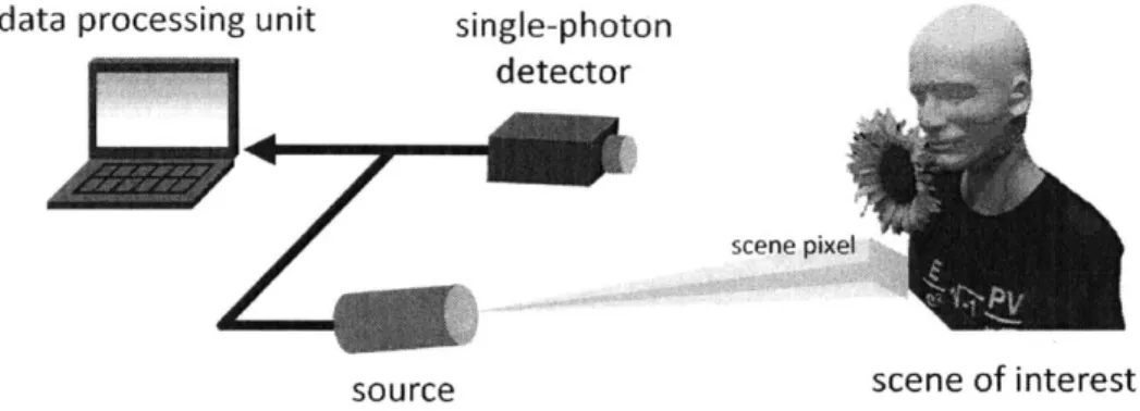
1-1 Single-photon active imaging setup with common components. The figure specifically depicts a setup with scanning source and a single-pixel detector. . . . . 30

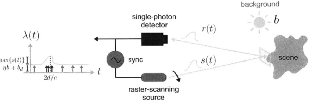
,2-1 An illustration of the data acquisition procedure for one illumina-tion pulse. A pulsed optical source illuminates a scene pixel with photon-flux waveform s(t). The flux waveform r(t) that is incident on the detector consists of the pixel return as(t - 2d/c)-where a is the pixel reflectivity, d is the pixel depth, and c is light speed-plus the background-light flux b. The rate function A(t) driving the photode-tection process equals the sum of the pixel return and background flux, scaled by the detector efficiency q, plus the detector's dark-count rate

bd. The record of detection times from the pixel return (or background

light plus dark counts) is shown as blue (or red) spikes, generated by the Poisson process driven by A(t). . . . . 36

2-2 Illustration of S2. Our non-convex union-of-subspaces constraint set

describes model-based signal sparsity that is specific to the LIDAR im aging setup. . . . . 39

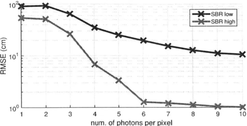
2-3 Simulation of pixelwise depth imaging results using single photon ob-servations for two SBR levels. (a) Depth RMSE of log-matched filter and proposed method for SBR = 200. (b) Depth RMSE of log-matched filter and proposed method for SBR = 100. . . . . 43

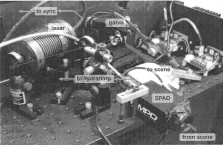
2-4 Experimental setup with a raster-scanning source and a single SPAD detector. The red arrows show the path of the optical signal from laser source, and the green arrows show the path of the electrical signal that indicates whether a photon has been detected or not. . . . . 44

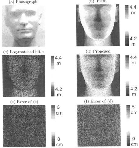
2-5 Experimental pixelwise depth imaging results using single photon ob-servations. The number of photon detections at every pixel was set to be 15. The figure shows the (a) photograph of imaged face, (b) ground-truth depth, (c) depth from log-matched filtering, which is approximately ML and (d) depth using our method. The absolute depth-error maps for ML and our framework are shown in (e) and (f), respectively. . . . . 45

2-6 Depth recovery performance of our algorithm at a -face pixel (SBR 6.7 and pixel coordinates (81,272)) and a depth boundary pixel (SBR = 1.5 and pixel coordinates (237, 278)) for varying number of photon detections. . . . . 46

3-1 Examples of active imaging scenarios in which the scene response is a sum of responses from multiple reflectors. (a) Imaging scene with a partially-reflecting object (shown in gray dashed line). (b) Imaging scene with a partially-occluding object. . . . . 50

3-2 (Top) Full-waveform single-photon imaging setup for depth estimation of multiple objects. In this example, a pulsed optical source illumi-nates a scene pixel that includes a partially-reflective object occluding a target of interest. The optical flux incident at the single-photon detector combines the backreflected waveform from multiple reflectors in the scene pixel with extraneous background light. (Bottom left) The photon detections, shown as spikes, are generated by the N8-pulse rate function NSA(t) following an inhomogeneous Poisson process. The green and blue spikes represent photon detections from the first and second reflector, respectively; the red spikes. represent the unwanted photon detections from background light and dark counts. (Bottom right) Our convex optimization processing enables accurate reconstruc-tion of multiple depths of reflectors in the scene from a small number of photon detections. . . . . 53

3-3 Illustration of a shrinkage-thresholding operation used as a step in ISTA (left) and the shrinkage-rectification operation used as a step in our SPISTA (right) that includes the nonnegativity constraint. Here the operations map scalar v to scalar z (variables only used for illus-tration purposes), with regularization parameter T. . . . . 57 3-4 Illustration of steps of Algorithm 3 using experimental photon-count

data for the single-pixel multi-depth example of partially-occluding reflectors in Fig. 3-9. (a) The raw photon count vector y from a pixel that contains two reflectors at around time bins 2600 and 3500. Other than the photon detections describing the two targets of interest, we observe extraneous photon detections from background and dark counts. (b) The output solution of SPISTA in Algorithm 2. Note that the extraneous background and detector dark counts are suppressed. (c) The final solution of Algorithm 3 that groups depths of SPISTA output. . . . . 60

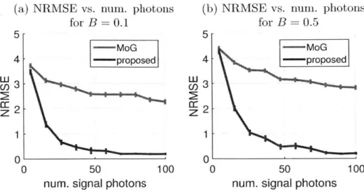
3-5 Simulated performance of MoG-based method and proposed frame-work of Algorithm 3 in recovering signals with K = 2 for two different

background levels. Signal photon detections are detections originat-ing from scene response and do not include the background-light plus dark-count detections. Note that the units of NRMSE are in meters, after being normalized by the pulsewidth; 1 NRMSE corresponds to an unnormalized mean-squared error of cTp/2 = 4.5 cm. The plots also include error bars indicating the 1 standard errors. . . . . 61

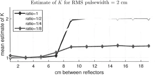
3-6 Simulated results of mean estimates of the number of reflectors pro-duced by Algorithm 2 at a pixel, when the RMS pulsewidth is set to gi-ve cT, = 2 cm. Here we show plots when the reflectivity ratio be-tween the first and second target is (a) 1 (blue line), (b) 1/2 (sky blue line), (c) 1/4 (yellow line), and (d) 1/8 (red line). . . . . 63

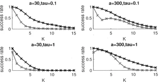
3-7 For different values of signal amplitude a (reflectivity multiplied by the peak value of pulse waveform) and regularization parameter r, the plots show success-1 in black and success-2 in red. Note that, by definition, success-1 upper-bounds success-2. . . . . 64

3-8 (Left) Photograph of the mannequin placed behind a partially-scattering object from the single-photon imager's point of view. (Right) Experi-mental results for estimating the mannequin's depth map through the partially-reflective material using MoG-based and our estimators, given that our imaging setup is at z = 0. The EM algorithm for MoG fit-ting used K = 2. Our multi-depth results were generated using the parameters TF= 0.1, 6 = 104 , E = 0.1, and 0 S y. . . . . 67 3-9 Single-photon imaging setup for estimating multi-depth from partial

occlusions at depth boundary pixels. Sample data from 38 photon de-tections is shown below for the pixel (94, 230) where partial occlusions occur. We show experimental results of multi-depth recovery for this

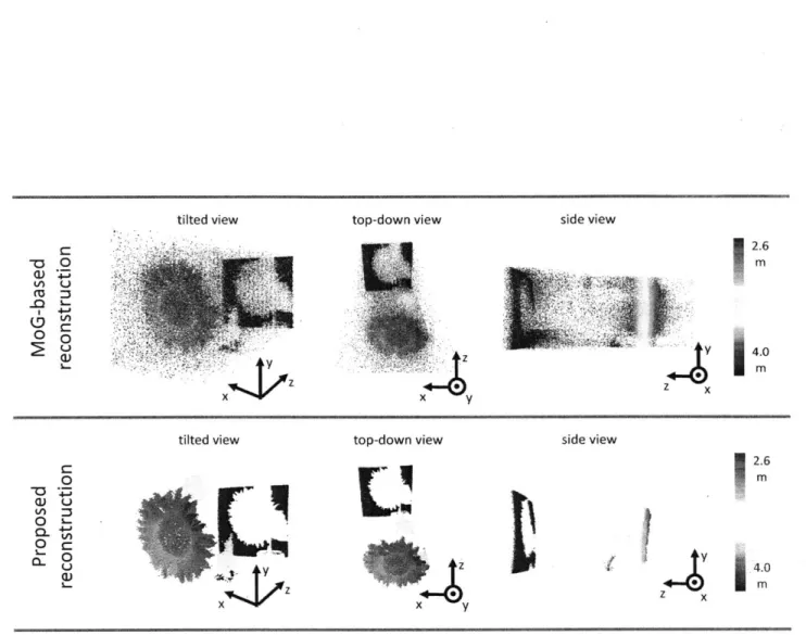
3-10 Experimental results of depth reconstruction for a sunflower occluding a wall, given that our imaging setup is at z = 0. Using our imaging framework, the mixed-pixel artifacts at the depth boundary of the flower and background light plus dark count noise are suppressed. The EM algorithm for MoG fitting used K = 2. Our multi-depth results were generated using the parameters T = 0.2, 6 = 10-4, c = 0.1, and

S=STy. ... ... ... ...71

4-1 Single-photon array imaging framework. (a) SPAD-array imaging setup. A repetitively-pulsed laser flood-illuminates the scene of interest. Laser light reflected from the scene plus background light is detected by a SPAD camera. Photon detections at each pixel are time tagged rel-ative to the most recently transmitted pulse and recorded. The raw photon-detection data were processed on a standard laptop computer to recover the scene's 3D structure and reflectivity. (b) Example of

3D structure and reflectivity reconstruction of mannequin and flower scene using the baseline single-photon imager from [1]. (c) Example of 3D structure and reflectivity reconstruction of mannequin and flower scene from our processing. Large portions of the mannequin's shirt and facial features that were not visible in the baseline image are revealed using our method. Both results in (b) and (c) were generated using an average of ~1 detected signal photon per pixel. . . . . 75

4-2 Photon-count histograms after censoring extraneous detections for the state-of-the-art pseudo-array method [21 (red) and our method (blue). The raw-data photon histogram is also given for reference (dashed black). The blue block indicates the ground truth depth values of objects in the scene scaled by c/2. By exploiting the scene's longi-tudinal sparsity, our method rejects more extraneous detections than does the pseudo-array method, which relies on transverse correlations. The greater the number of extraneous detections that survive censor-ing, the greater the amount of regularization that will occur in depth estimation, which will lead, in turn, to oversmoothing the depth image. 82

4-3 Stages of 3D structure and reflectivity reconstruction algorithm. (a) Raw time-tagged photon detection data are captured using the SPAD camera setup. Averaged over the scene, the number of detected signal photons per pixel was ~1, as was the average number of background-light detections plus dark counts. (b) Step 1: raw time-tagged photon detections are used to accurately estimate the scene's reflectivity by solving a regularized optimization problem. (c) Step 2: to estimate 3D structure, extraneous (background-light plus dark-count) photon detections are first censored, based on the longitudinal sparsity con-straint of natural scenes, by solving a sparse deconvolution problem. (d) Step 3: the uncensored (presumed to be signal) photon detections are used for 3D structure reconstruction, by solving a regularized op-timization problem . . . . . 84

4-4 3D structure and reflectivity reconstructions of the mannequin and flower scene. (a)-(d) Results of imaging 3D structure and reflectivity using the filtered histogram method, the state-of-the-art pseudo-array imaging method, our proposed framework, and the ground-truth proxy obtained from detecting 550 signal photons per pixel. For visualiza-tion, the reflectivity estimates are overlaid on the reconstructed depth maps for each method. The frontal views, shown here, provide the best visualizations of the reflectivity estimates. (e)-(h) Results of imaging 3D structure and reflectivity from (a)-(d) rotated to reveal the side view, which makes the reconstructed depth clearly visible. The fil-tered histogram image is too noisy to show any useful depth features. The pseudo-array imaging method successfully recovers gross depth features, but, in comparison with the ground truth estimate in (h), it overestimates the dimensions of the mannequin's face by several cm and oversmooths the facial features. Our SPAD-array-specific method in (g), however, gives high-resolution depth and reflectivity reconstruc-tion at low flux. (i)-(k) The depth error maps obtained by taking the absolute difference between estimated depth and ground truth depth show that our method successfully recovers the scene structure with sub-pulse-width resolution of less than cA/2 ~ 6 cm, while existing methods fail to do so. . . . . 85

4-5 Effect of varying the regularization parameters in our 3D structure and reflectivity reconstruction algorithm for the mannequin and flower scene. The optimal parameter set was {rA, Tz} = {2.6, 4.3}. . . . . . 88

4-6 Imaging results for the watering can and basketball scene. Notice the stripes of the basketball being visible when using our method. .... 89

4-7 Calibration results for the SPAD camera and scene parameters. (a) A 32 x 32 image of photon counts when the SPAD camera observes a weakly-reflecting planar wall with the laser off (left) was used to generate a 32 x 32 binary mask indicating hot-pixel locations with white markers (middle). The hot pixel mask was obtained by thresholding the photon-count image with an appropriate threshold chosen from the photon-count histogram (right). (b) Laser pulse shape. Extraneous photon detections were suppressed by time-gating near the roundtrip delay to a 1 x 1 m calibration target. (c) The non-constant 384 x 384 background-light plus dark-count rate matrix B for the mannequin and flower scene. . . . . 91

4-8 Relationship between RMS pulse duration and depth-recovery accu-racy. (a) Plot of depth-recovery accuracy using our algorithm (Step 2 and Step 3) versus RMS pulse duration T, obtained by simulating a low-flux SPAD imaging environment with an average of 10 detected sig-nal photons per pixel and 390 ps time bins. Depth recovery is deemed a success at a pixel if estimated depth is within 3 cm of ground truth, and the depth recovery accuracy of a method is computed by the mean success rate over all pixels. (b) Ground-truth depth map used in the simulations. (c) Estimated depth map for T, = 0.3 ns. (d) Estimated depth map for Tp = 1.1ns. (e) Estimated depth map for T, = 2.4ns. When Tp is too short, there is a systematic bias in the estimated depths, although random errors are minimal. When T is too long, the esti-mated depths are very noisy. In all our SPAD-array experiments we used T ~ 1 ns, which is in the sweet spot between durations that are too short or too long. We emphasize, however, that our algorithm is not tuned to a particular pulse-width and can be performed using any

4-9 Photon efficiency of proposed framework. (a) Plots of RMS depth error (log scale) versus average number of detected signal photons per pixel for imaging the mannequin's face using our proposed framework and the baseline pixelwise processor. Our method consistently realizes sub-pulse-width performance throughout the low-flux region shown in the plot, whereas the baseline approach's accuracy is more than an order of magnitude worse, owing to its inability to cope with extraneous detections. (b) Summary of photon efficiency versus acquisition speed (not the computational speed) for existing 3D structure and reflectivity imagers, where fps denotes frames per second and ppp denotes photons per pixel. . . . . 95

5-1 (a) Scanning LIDAR setup. A repetitively pulsed source illuminates the scene in a scanning manner, where at each scan point multiple re-flectors at different depths may be illuminated. The detector records the photon-count histogram of the backreflected response. (b) From one scanning pixel to another, there can be overlap in illumination due to physical constraints. (c) The interpixel overlaps can come from either illumination non-idealities, such as its finite beam-width (top), or scene constraints such as the presence of strongly scattering me-dia that generate random speckle illumination patterns (bottom). We define the two-dimensional intensity pattern cast on the scene as the transverse imaging kernel in our problem, and denote it using the two-dimensional function h centered at (0, 0). . . . . 101

5-2 Illustration of the acquisition model when imaging a one-dimensional scene. The PSF from scene illumination is modeled by H and the temporal pulse waveform and detector response is modeled by S. Both H and S are Gaussian convolution matrices in this example. B models the extraneous background and detector dark count response. The set of photon-count histograms observed at each scan pixel after N,

illumination trials is represented by Y. . . . . 103 5-3 Illustration of S1(N, m) for m = 3. Since every row of X E S1(N, m)

belongs to a set of 1-sparse signals, our constraint set S1(N, m) is a product space of N of 1-sparse signal sets. . . . . 104 5-4 Reflectivity reconstruction results (with mean absolute errors (MAE))

for a 19 x 19 MIT logo scene when SBR = +oo. We compare the pixel-wise ML, deconvolved ML, and the proposed frameworks (Approach 1 and 2) for different PSFs and values of signal photons per pixel (sppp). (b-e) Using Gaussian PSF and sppp = 106. (f-i) Using Gaussian PSF and sppp = 104. (j-n) Using Bernoulli PSF and sppp = 103. (n-q) Using Bernoulli PSF and sppp = 102 ... 114 5-5 Depth reconstruction results (with mean absolute errors (MAE)) for a

19 x 19 MIT logo scene when SBR = +oo. We compare the pixelwise ML, deconvolved ML, for different PSFs and values of signal photons per pixel (sppp). (b-e) Using Gaussian PSF and sppp = 106. (f-i) Using Gaussian PSF and sppp = 104. (j-m) Using Bernoulli PSF and Sppp = 103. (n-q) Using Bernoulli PSF and sppp = 102. . . . . 115 5-6 Reflectivity reconstruction results (with mean absolute errors (MAE))

for a 19 x 19 MIT logo scene when SBR = 1. We compare the pixelwise ML, deconvolved ML, and the proposed frameworks (Approach 1 and 2) for different PSFs and values of signal photons per pixel (sppp). (b-e) Using Gaussian PSF and sppp = 106. (f-i) Using Gaussian PSF and sppp = 104. (j-m) Using Bernoulli PSF and sppp = 103. (n-q) Using Bernoulli PSF and sppp = 102. . . . . 116

5-7 Depth reconstruction results (with mean absolute errors (MAE)) for a 19 x 19 MIT logo scene when SBR = 1. We compare the pixelwise ML, deconvolved ML, and the proposed frameworks (Approach 1 and 2) for different PSFs and values of signal photons per pixel (sppp). (b-e) Using Gaussian PSF and sppp = 106. (f-i) Using Gaussian PSF and

sppp = 10'. (j-m) Using Bernoulli PSF and sppp = 103. (n-q) Using Bernoulli PSF and sppp = 102 ... 117

5-8 Reflectivity and depth reconstruction results for a simulated ultra low-light LIDAR setup with MIT logo scene for SBR = +oo, with high native resolution of 270 x 275 (thus, N = 74250). Here, the mean number of photons per pixel was 9.8. We compare the pixelwise ML, ML after Richardson-Lucy (RL) deconvolution, and results of our Ap-proach 2 for both reflectivity and depth recovery. Here dmax is 18 cm. 120

5-9 Reflectivity and depth reconstruction results for a simulated ultra low-light LIDAR setup with MIT logo scene for SBR = 1, with high native resolution of 270 x 275 (thus, N = 74250). Here, the mean number of photons per pixel was 9.8. We compare the pixelwise ML, ML after Richardson-Lucy (RL) deconvolution, and results of our Approach 2 for both reflectivity and depth recovery. Here dmax is 18 cm. . . . . . 121

6-1 Active single-pixel imaging setup. For the kth measurement, the con-stant flux sent from source (s(t) = 1/Tr, t E [0, Tr)) and reflected from x is spatially-modulated using the pattern ak, such that the flux incident on the single-photon detector is afx. The observation

Yk ~ Poisson(aTx) is made by the photodetector, and the process is repeated for M measurements. Although this figure depicts the spatial light modulator as a reflector, such as a programmable mirror device, it may work in transmission mode by using a random diffraction grating instead. ... ... 125

6-2 Plots of EDFs fx(w) (x) for different q values according to the Marchenko-Pastur law . . . . . 130

6-3 Plots of logarithmic mse (dashed black with 'x' markers), mse-rmt (red with 'o' markers), and mse-baseline (blue with diamond markers) for different values of the Bernoulli probability p E {0.2, 0.5, 0.8} and sig-nal dimension N

C

6-4 Rice single-pixel camera setup. This photograph is taken from the Rice single-pixel camera project website: http: //dsp .rice .edu/cscamera.

134

6-5 Least-squares single-pixel imaging estimates of letter 'R' for increasing values of M using the Rice single-pixel dataset. Here, N = 16 x 16 = 256 and the ground truth image was generated using the least squares solution with Al = 4290, since it is an asymptotically efficient estim ator. . . . . 136

6-6 Comparison of MSE (plot in log scale) estimates for least-squares imag-ing method on experimental Rice simag-ingle-pixel camera data of letter 'R'. Here N = 16 x 16 = 256. . . . . 137

6-7 Plot of nrmse-rmt over Al and P for N = 50 and p = 0.5. The red line gives the contour for nrmse-rmt = 0.4. . . . . 138

7-1 Single-photon fluorescence imaging setup as described in Section 7-1 (Top) and an illustration of the photodetection process (Bottom). In this illustration, we have one photon detection (marked in red) result-ing from the (i, j)-th pixel's second pulse excitation of the fluorophore sample, given that N, = 3. Note that we define the start of the fluo-rescence process as time t = 2dij/c, which is defined by the calibrated

sample-to-imager distance. This distance offset in defining the decay signal does not affect the lifetime measurements, as exponential pro-cesses are memoryless. . . . . 144 7-2 Example large photon count histogram of A'(t) from a pixel of a

quan-tum dot sample with lifetime of -7 ns, used to visualize the properties of fluorescence signals. The total number of detections contains infor-mation about fluorescence intensity and the rate of decay of the his-togram contains information about fluorescence lifetime. The residual photon counts uniformly distributed over [0, 64) ns are the extraneous background and dark counts. . . . . 146 7-3 Experimental recovery results of (top) fluorescence intensity

normal-ized to have maximum value of 1 and (bottom) lifetime for two different quantum dot scenes with different mean numbers of photons-per-pixel (ppp) using the pixelwise maximum-likelihood estimator and the pro-posed framework. . . . . 152

B-1 Plots of probability function in Eq. (B.6) for different values of a. For increasing a, the probability function deviates away from the normal-ized rate function x shown as the dashed black line. . . . . 164 B-2 Plots of x (dashed blue line, labeled as "truth"), y/n, (solid black line,

labeled as "dead"), and iS,, (solid red line, labeled as "estimate"), which was obtained using Algorithm 7. . . . . 166 B-3 Plots of log-RMSE of y and fifx for increasing number of photon

E-1 SPAD-camera image acquisition terminology for RS-mode operation. 174 E-2 Experimental SPAD-array imaging setup. . . . . 178 E-3 Scanning scheme to obtain increased image area and image resolution

using the 32 x 32-pixel SPAD array. (a) Array translation by increments of a full array size (4.8 mm) along both axes to image multiple tiles of the entire array. (b) Zoom-in view of individual SPAD pixels showing the active area with no sub-pixel scanning, (c) 2 x 2 sub-pixel scanning by translating along each axis by 75 ptm, hence multiplying resolution by 2 in each dimension. . . . . 179 F-1 Depth variation vs. SNR. The solid blue line shows Eq. (F.7) and the

dashed red line indicates N , which is an upper bound to SNR, for various values of depth-var. . . . . 183

G-1 Plots of crb and mse generated using Monte Carlo simulations of Eq. (G.14) and Eq. (G.16). Observe that as Al increases, the crb becomes a tighter lower bound for mse. . . . . 188

List of Tables

3.1 Processing times for MoG and proposed methods for experimental imaging through a partially-reflecting object. . . . . 68 3.2 Processing times for MoG and proposed methods for experimental

Chapter 1

Introduction

Modern imaging systems enable us to better understand our physical environment by providing capabilities that exceed those of the human eye. Active imaging systems in particular use their own light sources and detectors to recover useful scene informa-tion, such as 3D structure, object reflectivity, fluorescence, etc. In order to suppress noise inherent in the optical sensing process, they usually require huge amounts of light to form their images. For example, a commercially available flash camera typi-cally collects more than 109 photons (103 photons per pixel in a 1 megapixel image) to provide the user with a single photograph [31. However, in sensing a macroscopic scene at a long standoff distance, as well as in imaging of microscopic biological samples, physical limitations on the amount of optical flux available and sensor integration time preclude the collection of such a large number of photons. In those cases, when the light incident on the detector is very low, we must resort to using sensitive single-photon imaging systems that are able to resolve individual single-photon detections. A key challenge in such scenarios is to make use of a small number of photon detections to accurately recover the desired scene information. Driven by such constraints, it is then natural to ask the following question: how many photons do we really need to form an image?

In this thesis, we address that question by investigating an imaging framework in which small numbers of photon detections are used as raw observations. Mainly, we show how computation and signal processing play an integral role in the

photon-efficient image formation process for the following imaging scenarios, which are well-known in the classical high light-level regime.

" Single-reflector depth imaging: Pulsed illumination onto an opaque, re-flective object leads to backscattered light, which is incident on the imager's detector. A time-resolved sensor is able to record the backreflected optical flux and use its time-of-flight information to infer the object depth on a pixel-by-pixel basis. This is the fundamental problem of light detection and ranging (LIDAR) [4].

* Multi-depth imaging: Pulsed illumination of a complicated scene produces reflections from many surfaces in a pixel, generating a complicated temporal profile for the light arriving at the detector. Using a time-resolved sensor, we can observe the combined response of the multi-reflections. Pixelwise reconstruction of multiple object depths by analyzing the combined response is the multi-depth imaging problem [5].

" Array-based time-resolved imaging: A detector array used for active scene 3D and reflectivity imaging typically suffers from low temporal resolution, because each detector element in the array can only be engineered to have a moderate sampling rate, as compared to those for single-detector-based scanning imagers. By mitigating this array-specific artifact, we can accurately reconstruct the scene's 3D and reflectivity characteristics from array measurements. This is the problem of array-based time-resolved imaging [6].

" Single-pixel imaging: When photodetectors are expensive, such as those operating at infrared or ultraviolet wavelengths or those capable of detecting individual photons, a single-pixel imaging system that reconstructs spatially-resolved reflectivity images using one photodetector, one source, and a spatial light modulator is a desirable imager [7].

" Super-resolution depth imaging: Spatial resolution of an active 3D imager is limited by its transverse pixelation degree. Is it possible to improve the spatial

resolution of the reconstructed depth map beyond the native pixel resolution? This is the problem of super-resolution depth imaging [8].

9 Fluorescence imaging: Fluorescent markers are used to label and track the locations of molecular processes or samples. The aim in fluorescence imaging is to recover spatially-resolved images of the sample fluorescence intensity and lifetime that give information about its molecular properties [9].

1.1

A Unifying Viewpoint

The single-photon active imaging setup has three common components for all of the previously described imaging scenarios. (See Figure 1-1 for an illustration of the setup.)

1. Source: The single-photon imaging setup includes a light source that illu-minates the scene with a temporally varying waveform, such as a pulse signal. The source can either be a laser that illuminates one pixel at a time as part of a raster-scanning process of the scene, or a floodlight source that sends out light to all pixels simultaneously.

2. Single-photon detector: Depending on the imaging application, we can either use a single-pixel photon counting detector or an array of single-photon detectors to record the detection times of individual photons arriving from the scene illuminated by a source.

3. Optics: Optical components such as lenses and spatial light modulators are often required to focus and control the light transport, in addition to the source and the single-photon detector.

We can then describe the common single-photon imaging setup employing those three components as follows. We use s(t) to denote the photon flux of a finite-duration waveform emitted into the scVne at time t = 0, and T, to denote its root mean square (RMS) duration. We take N to be the total number of pulses employed per pixel and

data processing unit single-photon detector

scene pixel

source scene of interest

Figure 1-1: Single-photon active imaging setup with common components. The figure specifically depicts a setup with scanning source and a single-pixel detector.

T, 1h the repetition period of the pulse itlumination. (See Appendix A for a complete table of notations used in this thesis.)

To build up our model for the photodetection statistics., it is convenient to restrict

our attention to a single scene pixel for now. Let I(t) be the scene impulse response function that we are interested in knowing at the particular J)ixel. For example,. 1(t)

is an impulse function when imaging a single reflector, a iulti--peaked function when

imaging an object through diffilse media, and a decaying expoiential function w ib

unknown lifetime when imaging target fluorescence. When s(t) iluimin ates the pixel

in question, the photon flux r(I) incident on the single-photon detector, is

where (s*)( t) is the convolution hetween the pulse waveform and the scene response, and 1(t) represents the unwanted background response, such as sunlight or light from a competing active imager. The rate function A(t) generating the photon detections at the single-photon detector is then

() * Ij)(t) + b, I

e

H.

where i/

e

Defin-ing 9(t) = (s * Id)(t) and b(t) = (b * Id)(t), we can rewrite Eq. (1.2) as A(t)

( * I)(t) + 'Ib(t) + bd.

A time-correlated single-photon detector is capable of determining the time-of-detection of a photon within an accuracy of A seconds. We assume A < T, and that T, is divisible by A. Then, we see that m = T/A is the number of time bins that contain our observed photon detection times. In other words, m is the size of the photon-count vector y, where Yk e {0, 1, 2, .. .} for k = 1, 2, ... ,m. Using the probabilistic theory of low-flux photon-counting, the number of photon detections in the kth time bin after N, pulse illuminations of a motionless scene is an integer random variable that is Poisson distributed:

Yk ~ Poisson N f A(t) dt , k = 1, 2,... , in (1.3) (k-1)A

where we have assumed that T, is long enough to preclude pulse aliasing and that b(t) is constant over the total acquisition time NsT,. Also, due to our low-flux assumption, the dead time effect of single-photon detectors is negligible (See Appendix B). The signal-to-noise (SNR) ratio, defined as the ratio of mean to the standard deviation, of the photon-count at kth bin is then

snr(yk) N A(t) dt, k =1,2, ... , m. (1.4)

We see that, as the number of illuminations increases, the signal-to-noise ratio also increases at a rate of N8. However, in order to operate in the regime of high

photon efficiency, we are interested in accurately recovering information about the scene response I(t) from single-photon observations y obtained using a small N,.

In order to form an image using a small number of photon detections, we propose a unifying photon imaging framework, which models the distribution of single-photon observations combined with physical constraints on scene parameters. Below we outline the elements of our framework, viz., the five-step procedure we will employ in all that follows.

" Step I: Derive the forward single-photon measurement model using the pho-todetection process from Eq. (1.3), for a specific single-photon imaging problem.

" Step II: Identify constraints on the scene parameters that we aim to recover. for the specific single-photon imaging problem.

" Step III: Combine the photodetection model and physical constraints derived in Steps I and II, respectively, to formulate an optimization program that solves the inverse problem of recovering the parameters of scene response I(t) (for a single pixel or multiple pixels, depending on the problem).

" Step IV: Regularize and relax the optimization problem that is formulated in Step III for computational efficiency, if necessary, while least perturbing the optimal solution.

" Step V: Design an algorithm that efficiently solves the final optimization prob-lem in Step IV.

We emphasize that our low light level imaging framework does not require any new optical technology, although it will certainly benefit from continued advances in single-photon detectors. Instead, it relies on the high computational power that can be made available in modern imaging systems. In the chapters that follow, we will apply our five-step framework for the single-photon imaging regime to the six imaging problems that were described earlier, and develop photon-efficient approaches for each of them.

Chapter 2

Single-Reflector Depth Imaging

2.1

Overview of Problem

A conventional LIDAR system, which uses a pulsed light source and a single-photon detector, forms a depth image pixelwise using the histograms of photon detection times. The acquisition times for such systems are made long enough to detect hun-dreds of photons per pixel for the finely binned histograms these systems require to do accurate depth estimation.

Prior art: The conventional LIDAR technique of estimating depth using his-tograms of photon detections is accurate when the number of photon detections is high, since the photon histogram can be considered as an observation of the backre-flected waveform. In the low photon-count regime, the depth solution is noisy due to shot noise. It has been shown that image denoising methods, such as wavelet thresh-olding, can improve the performance of scene depth recovery [101. In other work, an imaging model that incorporates occlusion constraints was proposed to recover an accurate depth map [11]. However, these imaging algorithms implicitly assume that the observations are either noiseless or Gaussian distributed. Thus, at low photon-counts, where photon-detection statistics are highly non-Gaussian, their performance degrades significantly [21.

imaging using only the first detected photon at every pixel. It demonstrated that centimeter-accurate depth recovery is possible by combining the non-Gaussian statis-tics of first-photon detection with spatial correlations of natural scenes. The FPI framework uses an imaging setup that includes a raster-scanning light source and a lensless single-photon detector. More recently, a photon-efficient imaging framework that uses a detector array, in which every pixel has the same acquisition time, has also been proposed [13, 141. It too relies on exploiting the spatial correlations of natural scenes.

We observe two common limitations that exist in the prior active imaging frame-works for depth reconstruction.

* Over-smoothing: Many of the frameworks assume spatial smoothness of the scene to mitigate the effect of shot noise. In some imaging applications, however, it is important to capture fine spatial features that only occupy a few image pixels. Using methods that assume spatial correlations may lead to erroneously over-smoothed images that wash out the scene's fine-scale features. In such scenarios, a robust pixelwise imager is preferable.

e Calibration: Many imaging methods assume a calibration step to measure the amount of background flux existing in the environment. This calibration mitigates bias in the depth estimate caused by background-photon or dark-count detections, which have high temporal variance. In practical imaging scenarios, however, the background response could vary in time, and continuous calibra-tion may not be practical. Furthermore, many methods assume background flux does not vary spatially. Thus, a calibrationless imager that performs simul-taneous estimation of scene parameters and spatially-varying background flux from raw photon detections is useful.

Summary of our approach: In this chapter, we propose a novel framework for depth acquisition that is applied pixelwise and without background calibration [15]. At each pixel, our imager estimates the background response along with scene depth

from photon detections. Our framework uses a Poisson observation model for the pho-ton detections plus a union-of-subspaces constraint on the scene's discrete-time flux at any single pixel, similar to the occlusion-based imaging framework in [11]. How-ever, our union-of-subspaces constraint is defined for both the signal and background waveform parameters that generate photon detections; whereas the framework in

[111

Using the derived imaging model, we propose a greedy signal pursuit algorithm that accurately solves for the scene parameters at each pixel. We evaluate the photon efficiency of this framework using experimental single-photon data. In the presence of strong background light, we show that our pixelwise imager gives an absolute depth error that is 6.1 times lower than that of the conventional pixelwise log-matched filter.

2.2

Single-Photon Imaging Setup

Figure 2-1 illustrates our imaging setup, for one illumination pulse, when the scene is illuminated in raster-scanning manner and a single-element photon detector is em-ployed. (Alternatively, to reduce the time needed to acquire a depth map, our frame-work can be applied without modification when the scene is flood illuminated and a detector array is used.) A focused optical source, such as a laser, illuminates a pixel in the scene with the pulse waveform s(t) that starts at time 0 and has root-mean-square pulsewidth Tp. This illumination is repeated every T, seconds for a sequence of N pulses. The single-photon detector, in conjunction with a time cor-relator, is used to time stamp individual photon detections, relative to the time- at which the immediately preceding pulse was transmitted. These detection times are observations of a time-inhomogeneous Poisson process whose rate function combines contributions from pixel return, background light, and dark counts. They are used to estimate scene depth for the illuminated pixel. This pixelwise acquisition process is repeated for N, x Ny image pixels by raster scanning the light source in the transverse directions.

bakrud

single-photon

b

A~t.)

y nu{ }sync ()scene

I\(t)

it

raster-scanning source

Figure 2-1: An illustration of the data acquisition procedure for one illuiination pulse. A pulsed optical source illuminates a scene pixel with photon-flux waveform s(O). The flux waveform r( ) that is incident on the detector consists of the pixel return (t - 2d/ where a is the pixel reflectivity, d is the pixel depth, and is light speed--- plus the background-light flux ). The rate function A(t) driving the photodetection process equals the sum of tle pixel return and background flux, scaled by the detector efficiency j., plus the detector's dark-count rate 1.j. The record of detection times from the pixel return (or background light plus dark counts) is shown as blue (or red) spikes, generated by the Poisson process driven by A().

2.3

Forward Imaging Model

In this section, we introduce a model relating photon detections and scene paranteirs. For simiplicity of exposition and notation, we focus on one pixel; this model is repeated for each I pixel of a raster-scanning or array-detection setup.

Let a f, danl /) he unknown scalar values that represent reflectivity. depth, and

background flux at the given pixel. The reflectivity value includes the effects of radial fall-offt view angle, and material properties. Then, after illuminating the scene pixel with a single pulse t), the backreflected waveform that is incident at the single-photon detector is

r )= s -2 / )+ , [,T ).(2.1)

Comparing to our general light transport equation in Eq. (1.1), Eq. (2.1) specifically assumes that the scene response is generated Iy a single reflector (1(t) is scaled and shifted Dirac delta function) and that the background light is constant.

Photodetection statistics: Using Eq. (2.1), we observe that the rate function that generates the photon detections is

A(t) = q (as(t - 2d/c) + b) + bd, t E [0, Tr), (2.2)

where q E (0, 1] is the quantum efficiency of the detector and bd ;> 0 is the dark-count

rate of the single-photon detector. Here, we have assumed an ideal detector response: Id(t) = 6(t)

Recall that A is the time bin duration of the single-photon detector. Then, we define m = Tr,/A to be the total number of time bins that capture photon detections. Let y be the vector of size m x 1 that contains the photon counts at each time bin after we illuminate the pixel N times with pulse waveform s(t). Then, from low-flux photon-counting theory in Eq. (1.3), we have that

Yk ~ Poisson (N,j [,r(as(t - 2d/c) + b) + bd] dt , (2.3)

for k = 1,..., m. Note that we have assumed a stationary reflector and that our total pixelwise acquisition time NsT, is short enough that b is constant during that period. We have also assumed that the low-flux condition E= Yk

<

effect of the single-photon detector's reset (dead) time can be neglected. We wish to reach an approximation in which the Poisson parameter of Yk is given by the product of a known matrix and an unknown (and constrained) vector.

Choose n E Z+ such that A' = T,/n is deemed adequate resolution for the esti-mated time of flight. (Our interest is in high-resolution imaging, where n ;> 'n, and

hence A' < A.) Since 2d/c G [0, T,.), v E R'rIxI defined by

N8'qa, if 2d/c E

[(j

v = 0 = 1,2,e.i..n, (2.4)

has exactly one nonzero entry. Using this vector,

N8?Ias(t - 2d/c) ~ vjs(t - (j -

)

j=1

is a good approximation when A' is small enough, because the sum has one nonzero term and 2d/c has been quantized to an interval of length A'. Substituting (2.5) into

the Poisson parameter expression in (2.3) gives

j=1(kA

Then, defining 1,,1 to be an m x 1 vector of 1's, we can rewrite (2.3) as

yk ~ Poisson( (Sv + Blmx1),k), (2.6)

for k = 1,... Im, where

(2.7)

(2.8)

Sij

(t

(')

B = Ns(qb + bil),

for i = 1 .. , im and

j

Yk ~ Poisson((Ax)k

_).

So far, we have simplified the pixelwise single-photon observation model, such that the photon-count vector y E N""' is a linear measurement of scene response vector x E R 1)xl corrupted by signal-dependent Poisson noise.

Scene parameter constraints: We defined our (n

+

3

S2

X

Figure 2-2: Illustration of S. Our non-convex union-of-subspaces constraint set describes model-based signal sparsity that is specific to the LIDAR imaging setup.

nonzero entry, x lies in the union of o subspaces defined as

S,

{x

X

where each subspace is of dimension 2. Figure 2-2 illustrates S, for o = 2.

2.4

Solving the Inverse Problem

Using accurate photodetection statistics and scene constraints, we have interpreted the problem of robust single-photon depth imaging as a noisy linear inverse problem, where the signal of interest x lies in the union-of-subspaces Sa. Using (2.9), the observed photon count histogram y has the probability mass function

Thus, neglecting terms in the negative log-likelihood function that are dependent on

y but not on x, we can define the objective function

(x; A, y) = [(Ax)k - Yk log (Ax)k.

(2.12)

k=1

This objective can be proved to be convex in x.

We solve for x by minimizing C(x; A, y) with the constraint that x lies in the union-of-subspaces S,. Also, because photon flux is a non-negative quantity, the minimization results in a more accurate estimate when we include a non-negative signal constraint. In summary, the optimization problem that we want to solve can be written as

minimize C(x; A, y) (2.13)

s.t. X S,

x11 ;>

O, i

+ 1).

To solve our optimization problem in which the union-of-subspaces selects a sparse support, we propose an algorithm that is inspired by an existing fast iterative algo-rithm for sparse signal pursuit.. Compressive sampling matching pursuit (CoSaMP) [161

is a greedy algorithm that finds a K-sparse approximate solution to an underdeter-mined linear inverse problem. CoSaMP iterates until it finds a solution that agrees with the observed data (according to some convergence metric), while the solution is a linear combination of K columns of the forward matrix A. Adapting CoSaMP to our imaging framework is interesting for two particular reasons. First, unlike algorithms that only add to the solution support, never culling, CoSaMP has solution stability and accuracy properties that compete with globally-optimal fi-based convex opti-mization methods for sparse approximation [171. Second, CoSaMP has been shown to be adaptable to applications in which the signal being estimated has a structured support [181, as is true for the union-of-subspaces model. Thus, we are motivated to modify the CoSaMP algorithm to our specific use case, where we are interested in

recovering a sparse solution in the union-of-subspaces SN, instead of a K-sparse one, using photon-noise corrupted data.

Algorithm 1 Single-photon depth imaging using a union-of-subspaces model

Input: y, A, 6 Output: Ruos Initialize 5(') +

J,

Q +- supp((x':n)[l]) U supp(> ) U {n + 1} > Merge support

wIq <- AtQy, wloe -- 0

(k) --

'

u +- y - Ak(k) until ||(k-1) 1 - R(k) 1 1 <

kuos <- (k) c> Output converged solution

Our proposed greedy algorithm, inspired by CoSaMP, is given in Algorithm 1. We define 'To(x) to be the thresholding operator that sets all negative entries of x to zero, supp(x) to be the set of indices of x's nonzero elements, and X[k] to be the vector that approximates x with its k largest terms. Also, we take As to be a matrix generated using the columns of A described by the index set S. Finally, we use AT and At to denote the transpose and pseudo-inverse of matrix A, respectively.

In Algorithm 1, for computational efficiency we have approximated L(x; A, y) with the (2-loss fly - Ax11, which is the first-order Taylor expansion (up to a con-stant) of C(x; A, y) with respect to x (see Appendix D for derivation). Because CoSaMP also assumes an f2-loss function, the only change from CoSaMP to our al-gorithm is then the update stage; instead of picking out the best k terms, we pick out the two terms from the intermediate solution based on the union-of-subspaces and non-negativity constraints. We iterate the algorithm until the solution meets the convergence criterion: 1

)

Many sparse pursuit algorithms, such as CoSaMP, are successful given the as-sumption that A is incoherent. In our setup, however, the forward matrix A is

highly coherent due to A' being small and the pulse waveform s(t) being smooth. Nevertheless, because the linear system's degree of underdetermination is extremely mild (A E R (n + 0) and the sparsity level is fixed to a small number (dim(S.) = 2) relative to the signal dimension (typically exceeding 100), our single-photon imaging algorithm recovers the scene parameters of interest in a robust manner.

2.5

Results

Simulations: We simulated the single-photon imaging setup using Eq. (2.9) to study the performance of the proposed depth imaging method. It would be valuable to compare our imaging method with the ML estimator for scene parameters {a, d, b}. Unfortunately, due to nonzero background flux, ML estimation requires minimizing a non-convex cost function, leading to a solution without convergence and accuracy guarantees. Thus, zero background is assumed conventionally, even for data that is contaminated by background, such that the ML depth estimate reduces to the simple log-matched filter [191:

dM = arg max log STY . (2.14)

Note that this estimator is equivalent to a one-step greedy algorithm (where a union-of-subspaces constraint is irrelevant) of minimizing L(x; A, y) for a 1-sparse solution. We use (2.14) as the baseline depth estimator that is compared with our proposed estimator using the union-of-subspaces model.

Figure 2-3 shows the root mean square error (RMSE) of depth reconstruction at two different signal-to-background (SBR) levels. The SBR is defined as the ratio of the probability of a detection coming from signal to the probability of a detection coming from background light plus dark counts:

Z>(Sv),

SBR = V)k .I(B (2.15)