Envy and Hope

HAL Id: hal-00616993

https://hal-pjse.archives-ouvertes.fr/hal-00616993

HAL is a multi-disciplinary open access

archive for the deposit and dissemination of sci-entific research documents, whether they are pub-lished or not. The documents may come from teaching and research institutions in France or abroad, or from public or private research centers.

L’archive ouverte pluridisciplinaire HAL, est destinée au dépôt et à la diffusion de documents scientifiques de niveau recherche, publiés ou non, émanant des établissements d’enseignement et de recherche français ou étrangers, des laboratoires publics ou privés.

Envy and Hope

Xavier Fontaine

To cite this version:

Envy and Hope: Relevant Others’ Consumption and

Subjective Well-being in Urban India

∗

Xavier Fontaine

Katsunori Yamada

August 25, 2011

Abstract

This paper exploits a unique micro-level survey to investigate the relationship between subjective well-being and reference consumption in urban Indian. Using accurate computations of individuals’ reference consumption, we find that other’s consumption has a positive impact on subjective well-being. This result validates Hirschman’s view that information dominates envy in rapidly developing areas. Whereas envy seems to undermine the well-being impact of growth in economically-established countries, growth appears to have an important role in urban Indian. Our finding is robust to the way we define the reference level of consumption.

keywords: Subjective Well-being, India, Relative utility, Tunnel effects

JEL classification: D00, J28

∗_{We are grateful to Shinsuke Ikeda, Fumio Ohtake, and Yoshiro Tsutsui for permission for the usage}

of an unique data set of “Survey on Preferences toward, and Satisfaction with, Life" of Osaka University. We are also grateful to the CEPREMAP for providing us the Indian National Sample Survey data. We would like to thank Claudia Senik, Andrew Clark, Clément Imbert and the seminar participants at Paris School of Economics for their helpful comments. Any remaining errors are the sole responsibility of the authors.

†_{Corresponding author: Paris School of Economics. E-mail: fontaine@pse.ens.fr}

1

Introduction

An important amount of research has recently been devoted to enrich the relative consumption theory. The view that behaviour and well-being levels can be affected by the relative position individuals derive from their consumption levels appears indeed to be very challenging from an economist perspective. Therefore, a variety of approaches have been taken to explore this relative consumption hypothesis, ranging from empirical and experimental evaluations of its validity, to theoretical to empirical inquiries into the causes and consequences of such a phenomenon (see Clark et al. (2008) for a review).

Despite this rich corpus, twilight zones remain to be explored in this nascent field of research. While the literature abounds with investigations in economically developed countries, the role comparisons play in emerging economies and (less ad-vanced) developing countries is still insufficiently documented. This is especially true for India and China, whereas these two countries account respectively for 17 % and 19 % of the world population.

The present study aims at bridging this gap, providing evidences on the impor-tance of relative concerns in one of the biggest emerging country: India. This is done by using an original survey on subjective well-being and expenditure in urban India. When other studies on developing countries may have to cope with limited datasets, we follow Clark and Oswald (1996) and Luttmer (2005) by combining our data with an external, huge and representative survey on consumption and expenditure in In-dia. This allows us to compute accurate estimates of the prevailing expenditure level in the reference groups.

The main finding in this paper is in line with Hirschman’s conjecture about countries experiencing a rapid economic development (Hirschman and Rothschild (1973)). Namely, we find that, in urban India, one is better off when people around her consume more than she does. This finding confirms that ambition may dominate envy in rapidly growing areas, and brings some new lights to our understanding of the well-being impact of growth.

This paper is organized as follows. The next section provides a brief literature review and motivates our research. Section 3 presents our data set and empirical specification. Empirical results are shown in Section 4, and Section 5 concludes the paper.

2

Literature Review

2.1

Envy and ambition

The evidences accumulated during the last two decades gave birth to the general consensus that one’s well-being depend on how much people consume arround him. However, seeing people consuming more than me can either have a negative, or a positive impact. This depends on the relative strength of two underlying and opposed forces. The first one is envy: the higher the consumption level of people around me, the worse I feel. This theory has been introduced in the economic framework by Duesenberry (1949).

The second force goes the other way round, correlating positively others’ con-sumption and own well-being. The idea is that, in some contexts, an individual

may consider others’ consumption as a valuable information about his future level of consumption. In situations where the economic mobility is high, but where there is also a lot of uncertainty about future outcomes, seeing people like me becoming richer gives me an information about the probability that I’ll also become richer later. Anticipating this improvement in my living conditions makes me feel better today.

This informational effect of others’ consumption has been conceptualised by Hirschman (1973). It is often referred to as the tunnel effect, due to Hirschman’s metaphor where a driver, stuck in a traffic jam in a two-lanes tunnel, feels better when seeing cars beginning to move again in the other lane. Even if everybody is still stuck in the same lane as our driver, he is pleased because he thinks that his turn will come soon.

2.2

Overall impact of other’s consumption

Which of envy and information/ambition dominates the other is highly context-dependent. The informational value of others’ consumption is expected to be higher in countries whose economic structures change rapidly, and that are characterised by important opportunities and strong uncertainty. In these countries, information may be expected to outweigh envy. In economically established countries, the contrary can be expected.

In line with these presumptions, most of the studies on developed countries report that the consumption level in the reference group impacts subjective well-being negatively, irrespective of the way one define the reference group. A rich review of this literature can be found in Clark et al. (2008). Very recently, Card et al. (2010) exploited a natural experiment setting to disentangle the respective roles of envy and information among Californian working in universities. Consistently with the previously quoted literature, they found that envy outweigh information, so that the overall impact of other’s income is negative.

When turning to Eastern-European, formerly communist countries, the picture changes radically. The collapse of the communist bloc lead to dramatic changes in social institutions and market structures, creating a lot of opportunities, but also a lot of uncertainty. In this context, one can expect the informational effect to be prevailing. The evidences support this guess: in her 2004 paper, Senik used a Russian panel survey to show that subjective well-being is positively correlated to others’ income during the 1994-2000 period.

She extends her study to other post-transition countries, including Hungary, Baltic countries, Poland, Latvia, Estonia, and Lithuania (Senik (2008)). Again, she finds the same kind of relationship, strengthening the support of Hirschman’s conjecture in transition countries.

The "less developed countries" form a very heterogeneous group, with respect to social mobility and uncertainty. For this reason, no overall conjecture can be made about the relative strengths of envy and ambition. Despite the rareness of the data in these countries, some authors managed gauge the importance of relative concerns in some of them, revealing mostly that envy is also of importance in the less developed countries (see Clark and Senik (2011) for a review).

Notwithstanding the variety of situations in these countries, some quite homo-geneous subgroups can be elicited. India and China form one of them, with annual

average growth rates of respectively 7.4 % and 10.4 % over the last decade, and popu-lations of 1.2 and 1.3 billions. In both countries, growth carries a lot of opportunities, especially in urban areas. In Indian, growth has been shown to be sustainable — to the sense of Arrow et al. (2003) — for five other decades (Sato et al. (2011)). For these reasons, one could expect the prevalence of a strong Hirschman effect in these two countries. Also, we can expect the informational effect to be stronger in urban areas.

So far, the lack of subjective well-being data hindered the research on comparison in India and China. To the best of our knowledge, only two papers make use of survey data to assess the role of group consumption in these countries, and both of them concentrate on rural areas. While Linssen et al. (2011) found that envy is dominating, Knight et al.’s study (2009) revealed both envy and ambition, depending on the specification. In this context, further investigations in India are welcome, especially in rapidly growing urban areas.

3

Model and Data

3.1

Model specification

As usual in the literature (Clark et al. (2008)), we model welfare as a function of log-expenditure, and of the log-reference level of expenditure. To be more precise, we specify the welfare function U as:

(1) Ui = α + ln(expi)βexp+ ln(ref expi)βref exp+ Xiγ + εi

expbeing monthly household expenditure per capita, while ref exp is the median of household expenditure per capita in the reference group. The Xs are other important socio-economic characteristics: age, sex, caste, marital status, number of children, labor force status, education, city.

The choice of the median instead of the average is motivated by one of its prop-erty, which is to be less sensitive to outliers (this point has been made by Clark et al. (2009)). As a matter of fact, replacing the median by the average in estimations does not substantively change the magnitude of ˆβref exp, but increases its standard-error as can be expected.

Because well-being statement are a discrete measure of the underlying and unob-servable welfare level U , our estimations are based on an ordered logit specification. However, and as often the case (Ferrer-i-Carbonell and Frijters (2004)), assuming that well-being statements are cardinal instead of ordinal (i.e. using ordinary least squares instead of an ordered probit) does not change the results substantively.

3.2

Defining the reference group

"People like me" are usually defined as those individuals who share some important characteristics with the respondent (social proximity), and who live or work close to her/him (geographical proximity). In most empirical studies, social and geographical proximities are used jointly to define the reference group, even though some papers consider only the former (e.g van de Stadt et al. (1985)) or the latter (e.g. Luttmer (2005)).

Here, both dimensions have been taken into account. More precisely, the refer-ence groups have been defined accordingly to four criteria. The first three of them are those used by Ferrer-i-Carbonell (2005): education, age and geographical loca-tion. Because India is endowed with a strong social hierarchy, caste has been added to this list. Alternative specifications are tested in section 4.3.

Education is defined accordingly to seven categories: illiterate ; literate but no formal schooling ; primary ; middle/upper primary; secondary/higher secondary ; college, but not graduate ; graduate and above. The age distribution has been divided into three groups, each one containing one-third of the adult population of the cities we study: 18-28 ; 29-40 ; 41 and above. The six cities are: Delhi ; Mumbai ; Bengaluru ; Chennai ; Kolkata ; Hyderabad. Finally, the three castes are the Scheduled Castes ; the Other Backward Classes ; and the "Other" (that is, those that belongs neither to Scheduled Castes or Tribes, nor to an Other Backward Class). 1 _{Altogether, these categories produce 378 cells.}

Studying the impact of reference consumption implies the inclusion of a set of dummies for each characteristic we use to define the reference group. The average expenditure level prevailing in a city may well be correlated to the level of public services, for instance ; this level of public services is very likely to be positively corre-lated with well-being. Not including these dummies could lead to serious endogeneity problems.

3.3

Data description

The present study uses two datasets jointly. The first one, the Osaka database (here-after ODB), surveyed about 1800 people in India in 2008, asking them subjective well-being and household expenditure questions, among others.2 _{The second one is} the Indian National Sample Survey (NSS), a huge representative survey driven by the Indian government. The NSS surveyed about 570,000 Indians in 2007-08. We used the NSS to compute in each reference group the median household expenditure per capita.

The Osaka database ("Survey on Preferences toward, and Satisfaction with, Life") is a longitudinal survey, conducted by the University of Osaka. Three waves of Indian data have been collected: 2008, 2009 and 2010. The first wave covered 1 800 adults in six big cities, drawing respondents randomly (with quotas) in each city. the two following waves surveyed the same individuals.

Obviously, using the ODB to estimate the reference levels of expenditures would be nonsense, due to the limited sample size. For this reason, we use an external representative, sizeable and good quality dataset to compute these reference levels. The National Sample Survey, started by the Indian government, in 1950, is an old institution, cumulating 64 rounds. It uses elaborated sampling methods to cover the whole Indian territory. In the six cities the ODB surveyed, the National Sample Survey covered 18 700 people (13 400 adults) in 2007-2008.

1

The Scheduled Tribes represent at most 2% of the population in the cities we have at hand. As a consequence, they are not considered in the present study.

2

Using the same data set, Ito et al. (2011) investigated the determinants of individual preferences for income redistribution in India. They showed that relatively wealthy individuals are more likely to favor greater redistribution. Their focus was on altruistic preferences and re-distribution policy in India, and was not related to relative utility issues which is the main focus of this paper.

At the time we are writing, we cannot use the last waves of the NSS. Thus, we are not able use the longitudinal dimension of the ODB, as it would require at least one more year of NSS data. For this reason, we only take benefit of the first year of the ODB. Exploiting the panel dimension of the ODB is left to further versions of this paper.

As said previously, there are 378 reference groups. In the NSS, there are on average 37 individuals in each of these cells. This number increases to 77 if we consider only the cells to which at least one respondent from the ODB belongs (i.e. the cells used in the regressions). This allows us to compute quite accurate estimates of the reference levels of expenditure in each group.

4

A strong tunnel effect

4.1

Impact of reference group expenditures

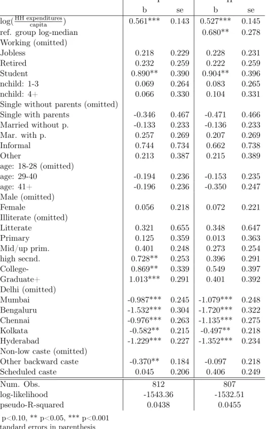
Table 1 provides the results for two specifications. The first one omits the reference level of expenditure, while the second includes it.

Ui = α + ln(expi)βexp +Xiγ+ εi (I)

Ui = α + ln(expi)βexp+ ln(ref expi)βref exp +Xiγ+ εi (II)

In specification (I), the level of expenditure has a positive and strongly signif-icant (to a 1 % level) impact on subjective well-being. This effect stays the same when adding the reference level of expenditure. The impact of the reference level of expenditure is also positive, and significant to a 2.5 % level. ˆβref exp appears to be bigger than ˆβexp, even though their ratio does not statistically differ from 1.

This result strongly supports the presumption that there exist a tunnel effect in the emerging India, and that this tunnel effect rules out envy. This informational effect of others’ consumption appears to be as strong as the impact of own consump-tion. This actually means that an individual benefits twice more from an increase in its consumption when people like him increase their consumption in the same pro-portion. This result contrasts sharply with what is usually found in most developed countries, where an homogeneous increase in the level of consumption prevailing in a group often results in an absence of well-being improvement.

4.2

Other covariates

Most of the other covariates (the number of children, marital status, age, and gender) are found to have significant impact on subjective well-being in both regression (I) and regressions (II). Several specifications have been tested for both the number of children and the age categories, without leading to a substantial significance increase. Some educational and caste dummies have a significant impact in the first regression, but not in the second.

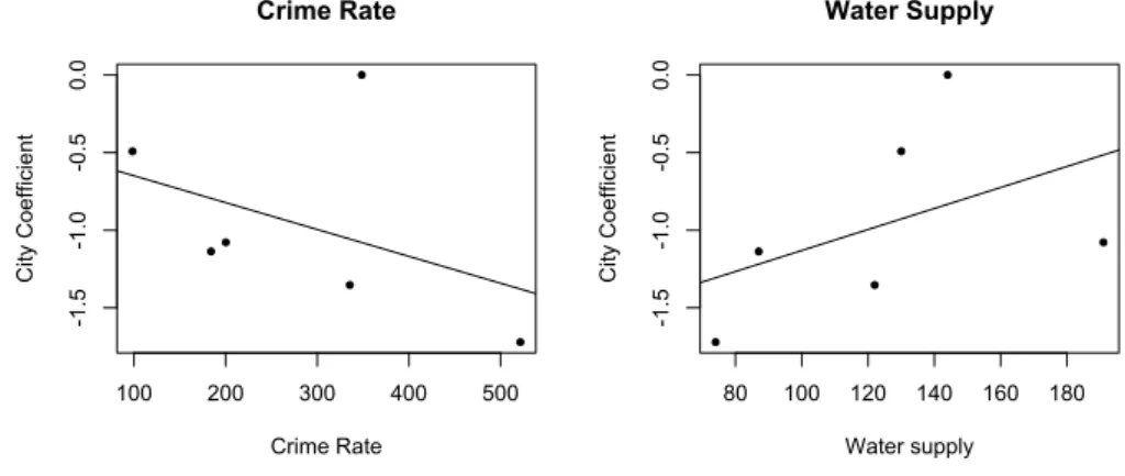
Individuals are happier when they are student than when they belong to any other labour force category. A fallaciously astonishing result is that jobless people don’t seem to be worse off than workers. This is explained by the fact that, accordingly to the NSS, the jobless category mostly consists of housewives and househusbands. City dummies have a strongly significant impact, irrespective of the regression considered. Interestingly, the associated coefficients fit very well to the knowledge

we have about each of these cities. Graph 1 shows the relationship between city coefficients on one hand, and both crime rate and water supply on the other hand. The correlation between city coefficients (from regression II) and crime rates is -0.41. The correlation between city coefficients and the level of water supply is 0.46. 3

Figure 1: Relationship between the city-specific coefficients in SWB equations, and city observable characteristics 100 200 300 400 500 -1 .5 -1 .0 -0 .5 0 .0 Crime Rate Crime Rate C it y C o e ff ici e n t 80 100 120 140 160 180 -1 .5 -1 .0 -0 .5 0 .0 Water Supply Water supply C it y C o e ff ici e n t

4.3

Robustness checks

The trustworthiness of our main result is checked along several lines. First, we ad-dress the concern that the positivity of the relationship between happiness and the reference level of expenditure may not be robust to the way the reference group is specified. To do so, we test all the possible combinations of the edu-cation/age/city/caste variables to define the reference group (education-age-city, education-age-caste, education-age, . . . ), and check whether we find some negative and significant coefficient. The impact of the reference level of expenditures appears to be positive and 10% - significant in one case (education-city-caste, with ˆβexp = .54 and ˆβref exp = .66), and insignificant in all the other cases.4

The logarithmic specification of the relationship between (own and reference group) expenditures and well-being can also be questioned. For that reason, we also check if our results are consistent when using a second-order polynomial specification instead of a logarithmic one, to allow for concave, convex and linear shapes. Again, we find concave, positive and significant impacts for own and others’ expenditures.

3

The crime rate data are those made available by the Ministry of Home Affairs (National Crime Records Bureau (2008)). Water supply is measured in litters per day per capita. Two reports, using the same methodology, have been combined to get water supply data for all the cities we have at hand: one from the Indian Ministry of Urban Development (2010), and the other one from the Asian Development Bank (2007).

4

When defining the reference group accordingly to only one variable, we have to drop the dummies related to the reference group in order to avoid colinearity problems. In that case, we have to cluster accordingly to the reference group variable. The results are unsingnificant. Remark that, in our case, this type of regressions does not make much sense, since the reference level of expenditure takes at most 6 values when the reference group is defined accordingly to a single variable.

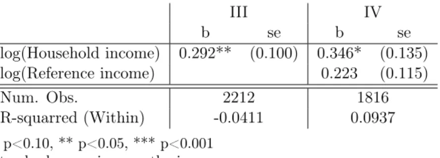
Another important robustness check is achieved by using individuals’ state-ments_{about how much others earn around them. The Osaka survey includes the} fol-lowing question: "About how much household income is common for people around you?". This question follows directly an annual household income question. We estimates the two following equations:

Uit= αi+ ln(incit)βinc +Xitγ+ εit (III) Uit= αi+ ln(incit)βinc+ ln(ref incit)βinc exp +Xitγ+ εit (IV)

where inci stands for the annual household income level, and ref inci is the answer to the above question. Remark that, this time, we have added a time-dimension, and introduced individual fixed-effects. The ODB is indeed a panel survey (2 waves available so far). Unfortunately, and as already said, the 2009-2010 wave of the NSS is not available at the time this first draft is written, preventing us from running a panel analysis for equation (I) and (II). The next version of this paper will extend our results in this direction.

We estimate (III) and (IV) using fixed-effect OLS. The results are summarised in table 2. The log(reference income) coefficient is positive, with a t-stat of 1.94 (10% significance level, almost 5%). It’s very likely that the 5% significance level will be attained when we will introduce the third wave of the ODB in our panel analysis (i.e. in the next version of the present paper).

5

Conclusion

The well-being impact of economic growth is obviously a topic of utmost importance for economists. Concentrating on six rapidly growing cities in India, this paper aims at bringing some additional material into the reflexion. Using subjective well-being data, together with several measures of the reference level of expenditure, we find that the richer people "like me" or "around me", the happier I am. To put it differently, envy does not undermine the well-being benefits that people can derive from growth, or at least not as much as it does in economically well-established countries. Seeing other people becoming richer them appears to be a very valuable information in India. As a consequence, individuals indeed better off when they know their living conditions are going to improve.

One should not conclude from our results that positional motives — such as envy — are not driving consumption behaviours in India. People’s consumption is an important signal for me, but this does not mean that I won’t try to keep up with them. What can be learned from the present study is rather that envy has a noticeably lower impact than information in urban India.

The present analysis could be deepened using panel data methods, but this hasn’t be done so far for data availability reasons. Fortunately, we will be able to take benefit from additional waves of data for both the Osaka database and the National Sample Survey very soon. Using them jointly will allow for a deeper exploitation of the panel dimension of our data.

References

Arrow, K., P. Dasgupta, and K.-G. Maler (2003): “Evaluating Projects and Assessing Sustainable Development in Imperfect Economies,” Environmental &

Resource Economics, 26, 647–685.

Asian Development Bank(2007): “2007 Benchmarking and Data Book of Water Utilities in India,” Tech. rep., Asian Development Bank.

Card, D., A. Mas, E. Moretti, and E. Saez (2010): “Inequality at Work: The Effect of Peer Salaries on Job Satisfaction,” NBER Working Papers 16396, National Bureau of Economic Research, Inc.

Clark, A. E., P. Frijters, and M. A. Shields(2008): “Relative Income, Hap-piness, and Utility: An Explanation for the Easterlin Paradox and Other Puzzles,” Journal of Economic Literature, 46, 95–144.

Clark, A. E., N. Kristensen, and N. Westergård-Nielsen (2009): “Eco-nomic Satisfaction and Income Rank in Small Neighbourhoods,” Journal of the European Economic Association, 7, 519–527.

Clark, A. E. and A. J. Oswald (1996): “Satisfaction and comparison income,” Journal of Public Economics, 61, 359–381.

Clark, A. E. and C. Senik (2011): “Will GDP Growth Increase Happiness in Developing Countries?” IZA discussion paper.

Duesenberry, J. S.(1949): Income, Savings and the Theory of Consumer Behav-ior, Harvard University Press.

Ferrer-i-Carbonell, A. (2005): “Income and well-being: an empirical analysis of the comparison income effect,” Journal of Public Economics, 89, 997–1019. Ferrer-i-Carbonell, A. and P. Frijters (2004): “How Important is

Method-ology for the estimates of the determinants of Happiness?” Economic Journal, 114, 641–659.

Hirschman, A. O. and M. Rothschild (1973): “The Changing Tolerance for Income Inequality in the Course of Economic Development; with a Mathematical Appendix,” The Quarterly Journal of Economics, 87, 544–66.

Ito, T., K. Kubota, and F. Ohtake (2011): “Noblesse Oblige? Preferences for Redistribution among Urban Residents in India,” Osaka University, GCOE Discussion Paper Series, 183, 1–46.

Knight, J., L. Song, and R. Gunatilaka (2009): “Subjective well-being and its determinants in rural China,” China Economic Review, 20, 635–649.

Linssen, R., L. van Kempen, and G. Kraaykamp (2011): “Subjective Well-being in Rural India: The Curse of Conspicuous Consumption,” Social Indicators Research, 101, 57–72, 10.1007/s11205-010-9635-2.

Luttmer, E. F. P. (2005): “Neighbors as Negatives: Relative Earnings and Well-Being,” The Quarterly Journal of Economics, 120, 963–1002.

Ministry of Urban Development (2010): “Handbook of Service Level Bench-marking,” Tech. rep., Ministry of Urban Development.

National Crime Records Bureau (2008): “Crime in India 2008,” Tech. rep., Ministry of Home Affairs.

Sato, M., S. Samreth, and K. Yamada(2011): “A Numerical Study on Assess-ing Sustainable Development with Future Genuine SavAssess-ings Simulation,” Interna-tional Journal of Sustainable Development, Forthcoming.

Senik, C. (2004): “When information dominates comparison: Learning from Rus-sian subjective panel data,” Journal of Public Economics, 88, 2099–2123.

——— (2008): “Ambition and Jealousy: Income Interactions in the ’Old’ Europe versus the ’New’ Europe and the United States,” Economica, 75, 495–513. van de Stadt, H., A. Kapteyn, and S. van de Geer (1985): “The Relativity

of Utility: Evidence from Panel Data,” The Review of Economics and Statistics, 67, 179–87.

Table 1: Happiness regression: estimations without, and with objectively measured ref-erence group expenditures. Ordered probit.

I II

b se b se

log(HH expenditures_capita ) 0.561*** 0.143 0.527*** 0.145

ref. group log-median 0.680** 0.278

Working (omitted) Jobless 0.218 0.229 0.228 0.231 Retired 0.232 0.259 0.222 0.259 Student 0.890** 0.390 0.904** 0.396 nchild: 1-3 0.069 0.264 0.083 0.265 nchild: 4+ 0.066 0.330 0.104 0.331

Single without parents (omitted)

Single with parents -0.346 0.467 -0.471 0.466

Married without p. -0.133 0.233 -0.136 0.233 Mar. with p. 0.257 0.269 0.207 0.269 Informal 0.744 0.734 0.662 0.738 Other 0.213 0.387 0.215 0.389 age: 18-28 (omitted) age: 29-40 -0.194 0.236 -0.153 0.235 age: 41+ -0.196 0.236 -0.350 0.247 Male (omitted) Female 0.056 0.218 0.072 0.221 Illiterate (omitted) Litterate 0.321 0.655 0.348 0.647 Primary 0.125 0.359 0.013 0.363 Mid/up prim. 0.401 0.248 0.273 0.254 high secnd. 0.728** 0.253 0.396 0.291 College- 0.869** 0.339 0.549 0.397 Graduate+ 1.013*** 0.291 0.401 0.392 Delhi (omitted) Mumbai -0.987*** 0.245 -1.079*** 0.248 Bengaluru -1.532*** 0.304 -1.720*** 0.322 Chennai -0.976*** 0.263 -1.135*** 0.275 Kolkata -0.582** 0.215 -0.497** 0.218 Hyderabad -1.229*** 0.227 -1.352*** 0.234

Non-low caste (omitted)

Other backward caste -0.370** 0.184 -0.097 0.218

Scheduled caste 0.045 0.206 0.406 0.249

Num. Obs. 812 807

log-likelihood -1543.36 -1532.51

pseudo-R-squared 0.0438 0.0455

* p<0.10, ** p<0.05, *** p<0.001 Standard errors in parenthesis

Table 2: Happiness regression: estimations without, and with subjective measures of reference income. OLS with fixed-effects.

III IV b se b se log(Household income) 0.292** (0.100) 0.346* (0.135) log(Reference income) 0.223 (0.115) Num. Obs. 2212 1816 R-squarred (Within) -0.0411 0.0937 * p<0.10, ** p<0.05, *** p<0.001 Standard errors in parenthesis