Evaluation of cloud convection and tracer transport in a three-dimensional chemical transport model

(1)

HAL Id: hal-03116002

https://hal.archives-ouvertes.fr/hal-03116002

Submitted on 20 Jan 2021

HAL is a multi-disciplinary open access

archive for the deposit and dissemination of

sci-entific research documents, whether they are

pub-lished or not. The documents may come from

teaching and research institutions in France or

abroad, or from public or private research centers.

L’archive ouverte pluridisciplinaire HAL, est

destinée au dépôt et à la diffusion de documents

scientifiques de niveau recherche, publiés ou non,

émanant des établissements d’enseignement et de

recherche français ou étrangers, des laboratoires

publics ou privés.

Evaluation of cloud convection and tracer transport in a

three-dimensional chemical transport model

W. Feng, M. Chipperfield, S. Dhomse, B. Monge-Sanz, X. Yang, K. Zhang, M.

Ramonet

To cite this version:

W. Feng, M. Chipperfield, S. Dhomse, B. Monge-Sanz, X. Yang, et al.. Evaluation of cloud convection

and tracer transport in a three-dimensional chemical transport model. Atmospheric Chemistry and

Physics, European Geosciences Union, 2011, 11 (12), pp.5783-5803. �10.5194/acp-11-5783-2011�.

�hal-03116002�

(2)

Atmos. Chem. Phys., 11, 5783–5803, 2011 www.atmos-chem-phys.net/11/5783/2011/ doi:10.5194/acp-11-5783-2011

Atmospheric

Chemistry

and Physics

Evaluation of cloud convection and tracer transport in

a three-dimensional chemical transport model

W. Feng1, M. P. Chipperfield1, S. Dhomse1, B. M. Monge-Sanz1, X. Yang2, K. Zhang3, and M. Ramonet4

1_{NCAS, Institute for Climate and Atmospheric Science, School of Earth and Environment, University of Leeds, Leeds, UK} 2_{NCAS, Department of Chemistry, University of Cambridge, Cambridge, UK}

3_{Max-Planck-Institut f¨ur Meteorologie, Hamburg, Germany} 4_{LSCE/IPSL, CEA-CNRS-UVSQ, France}

Received: 2 September 2010 – Published in Atmos. Chem. Phys. Discuss.: 6 October 2010 Revised: 15 June 2011 – Accepted: 17 June 2011 – Published: 22 June 2011

Abstract. We investigate the performance of cloud

con-vection and tracer transport in a global off-line 3-D chem-ical transport model. Various model simulations are per-formed using different meteorological (re)analyses (ERA-40, ECMWF operational and ECMWF Interim) to diagnose the updraft mass flux, convective precipitation and cloud top height.

The diagnosed upward mass flux distribution from TOM-CAT agrees quite well with the ECMWF reanalysis data (ERA-40 and ERA-Interim) below 200 hPa. Inclusion of mi-dlevel convection improves the agreement at mid-high lati-tudes. However, the reanalyses show strong convective trans-port up to 100 hPa, well into the tropical tropopause layer (TTL), which is not captured by TOMCAT. Similarly, the model captures the spatial and seasonal variation of convec-tive cloud top height although the mean modelled value is about 2 km lower than observed.

The ERA-Interim reanalyses have smaller archived up-ward convective mass fluxes than ERA-40, and smaller convective precipitation, which is in better agreement with satellite-based data. TOMCAT captures these relative dif-ferences when diagnosing convection from the large-scale fields. The model also shows differences in diagnosed con-vection with the version of the operational analyses used, which cautions against using results of the model from one specific time period as a general evaluation.

We have tested the effect of resolution on the diag-nosed modelled convection with simulations ranging from 5.6◦×5.6◦ to 1◦×1◦. Overall, in the off-line model, the higher model resolution gives stronger vertical tracer trans-port, however, it does not make a large change to the

diag-Correspondence to: M. P. Chipperfield (m.chipperfield@leeds.ac.uk)

nosed convective updraft mass flux (i.e., the model results using the convection scheme fail to capture the strong vection transport up to 100 hPa as seen in the archived con-vective mass fluxes). Similarly, the resolution of the forcing winds in the higher resolution CTM does not make a large improvement compared to the archived mass fluxes.

Including a radon tracer in the model confirms the im-portance of convection for reproducing observed midlatitude profiles. The model run using archived mass fluxes trans-ports significantly more radon to the upper troposphere but the available data does not strongly discriminate between the different model versions.

1 Introduction

Cumulus cloud convection is one of the major processes that affects the dynamics and energetics of atmospheric circu-lation systems (Bechtold et al., 2001). Convection has to be parameterised in all general circulation models (GCMs) and most numerical weather prediction (NWP) models due to their coarse spatial resolution. The cumulus parameterisa-tion aims to represent/formulate the collective effects of sub-grid-scale clouds on mass, momentum, vorticity and tracer distribution in terms of grid-scale prognostic variables in nu-merical models (e.g., Arakawa, 1993).

There are two types of cumulus parameterisations used in large-scale models: (1) Convective adjustment schemes (e.g. Manabe et al., 1965) are used to simulate the effects of dry and/or moist convection by adjusting the lapse rates of temperature and moisture to specified profiles within the local grid column which oversimplifies the physical pro-cess (Emanuel, 1994). (2) Mass-flux schemes use a cloud model to explicitly calculate profiles of cumulus mass flux and thermodynamic variables (e.g., Tiedtke, 1989). Mass

(3)

5784 W. Feng et al.: Evaluation of cloud convection and tracer transport flux schemes have been more widely used in models because

they can provide an internally consistent representation of turbulent mixing, updraft dynamics, microphysics and tracer transport.

Off-line three-dimensional chemical transport models (CTMs) are widely used to study processes controlling tracer distributions in the atmosphere. Although most CTMs can reproduce the general features of tracer distributions, there are still large uncertainties in the model simulations. This is due to the complex set of processes in the model (e.g., chem-istry, photolysis, aerosol, large-scale advection, convection, dry/wet deposition, planetary boundary layer mixing, emis-sions) as well as the quality of meteorological analysis data used. The parameterisation of sub-gridscale transport pro-cesses in CTMs is particularly problematic. The two possi-ble approaches are (i) include a scheme in the CTM to diag-nose convection from the large-scale meteorological fields or (ii) read in information on convective transport (i.e. from the same source which provides large-scale winds). Approach (i) is necessary if only the large-scale meteorological fields are available. For example, the ECMWF does not routinely archive information on convection in their operational analy-ses, although they do for the lower resolution reanalyses such as ERA-40 and ERA-Interim. However, in approach (i) the CTM is attempting to diagnose convection from large-scale fields which may have already experienced its effects, i.e. they are already stabilised. Approach (ii) has the advantage that the CTM transport will be more fully consistent with the dynamics of the NWP model (or GCM) providing the mete-orological data. However, this approach still depends on the accuracy of the convection produced in the NWP system.

Mahowald et al. (1995) compared the performance of 7 different convection parameterisations within the same CTM. The schemes tested included two versions of the Tiedtke (1989) scheme. They found that tracer distributions in the CTM were very sensitive to the choice of convection scheme. They emphasised that their tests were not able to definitively determine if any scheme was better than the oth-ers though they found that the Tiedtke scheme generally per-formed well. Tost et al. (2006) tested a range of convection parameterisations within the framework of a general circula-tion model (GCM). As they were dealing with a GCM the focus was on investigating differences in the hydrological cycle and meteorology. In a later paper Tost et al. (2007) compared convection/lightning parameterisations within the same model. Recently, Tost et al. (2010) extended their stud-ies by investigating tracer transport. By comparing with cam-paign data they found the shorter the lifetime of a species, the larger the impact of different convection schemes. While longer lived species such as CO and O3varied by ±25 % with

different schemes, shorter lived species varied by ±100 %. Examples of off-line tropospheric CTMs which use archived convective mass fluxes include the Oslo CTM2 (Berntsen et al., 2006) and the related FRGSUCI model (Wild et al., 2004). These avoid the problem of availability of

convection information by producing their own forecast data by running a version of the ECMWF Integrated Forecast Sys-tem (IFS) model. As a variation on this approach, Aschmann et al. (2009) used archived ECMWF ERA-Interim convec-tive detrainment rates to model tracer transport in the upper troposphere. Their off-line model had a lower boundary at 330 K (about 10 km) and they used the archived detrainment rates in the upper troposphere (UT), along with an assumed tracer mixing ratio in the convective plume, to inject trac-ers into the lower model levels. This approach allowed them to reproduce observed profiles of CHBr3 and CH3I in the

tropical UT.

As part of the EU SCOUT-O3 project, Russo et al. (2011) and Hoyle et al. (2010) compared the treatment of convec-tion in global GCMs, global CTMs (including our default TOMCAT model) and regional mesoscale models. Russo et al. (2011) focused on the meteorology while Hoyle et al. (2010) compared the transport of short-lived species to and through the tropical tropopause layer (TTL). Their idealised model tracers had lifetimes ranging from 6 h to 20 days. The different models produced very different rates of transport of short-lived species to the TTL and there were also significant differences between the 5 CTMs considered, despite the fact they were all forced by ECMWF meteorol-ogy. Clearly the details of the models’ convection treatments are likely to play a key role in determining these different distributions of short-lived tracers in the TTL, however other model differences (e.g. resolution, advection scheme) may also play a role.

Therefore, a key uncertainty in tropospheric CTMs is the accuracy of modelled sub-gridscale transport by convection. In this paper we investigate the performance of cloud con-vection and tropospheric tracer transport in the TOMCAT 3-D CTM (Chipperfield et al., 1993; Chipperfield, 2006). We compare approaches which diagnose convection from the large-scale meteorological fields with using mass fluxes archived by NWP systems. Therefore, we are able to inves-tigate specific causes for the different performance of CTMs reported in Hoyle et al. (2010). For the diagnosed convection we investigate the impact of resolution on the modelled con-vection, the impact of different external forcing meteorology and surface data, and the use of different parameterisations. We evaluate the model by comparing diagnosed convective quantities with ECMWF reanalyses and observations, and by using radon as a model tracer.

Section 2 of this paper describes the TOMCAT CTM and modifications made for this study. Section 3 describes the meteorological data used to force the model and the obser-vations used to test the convection parameterisation. The model results are presented in Sect. 4 and further discussed in Sect. 5. Our conclusions are presented in Sect. 6.

(4)

W. Feng et al.: Evaluation of cloud convection and tracer transport 5785

2 Model and experiments 2.1 TOMCAT 3-D CTM

TOMCAT/SLIMCAT is an off-line 3-D CTM first described in Chipperfield et al. (1993). The TOMCAT version uses a hybrid σ -p vertical coordinate and the model has a vari-able horizontal resolution and vertical levels. Tracers are transported by resolved, large-scale advection, convection and parameterised mixing in the boundary layer. Hori-zontal winds, temperatures and specific humidity are spec-ified using ECMWF meteorological (re)analyses (ECMWF operational analyses, ERA-40 or ERA-Interim analyses). Vertical advection is diagnosed from the large-scale diver-gence field (Chipperfield, 1999, 2006). The model uses the Prather (1986) advection scheme which conserves second-order moments of transport tracers and uses vertical turbu-lent parameterisation of Holtslag and Boville (1993) for the boundary layer mixing. Versions of the model which contain detailed chemical and aerosol schemes (e.g. Breider et al., 2010) are based on the same dynamical framework.

The convection scheme in TOMCAT is based on Tiedtke (1989) which uses a bulk entraining plume-type cloud model for all convective types and assumes different entrainment and detrainment rates for different types of con-vection. In general the Tiedtke scheme considers three types of convection (deep, shallow, midlevel) and includes an un-saturated downdraft. Deep convection is driven by mois-ture convergence in the entire column. Shallow convection is driven by moisture convergence in the boundary layer, and the midlevel convection occurs when there is upward motion creating conditional instability (e.g., Tiedtke, 1989; Mahowald et al., 1997). The default TOMCAT convection scheme includes cumulus updrafts in the vertical column, entrainment of environmental air into the cloud and detrain-ment of cloud air to the environdetrain-ment (similar to the “Tiedtke-TM2” code tested by Mahowald et al., 1995). However, it does not include midlevel convection and convective down-drafts and there is no organised entrainment of environmental air above cloud base (see Stockwell and Chipperfield, 1999; hereafter SC1999).

Recently we have extended the options of moist convec-tion parameterisaconvec-tions in TOMCAT. We have updated the de-fault convection scheme to include midlevel convection and convective downdrafts. The entrainment and detrainment rates for the three types of convection use the same values as Tiedtke (1989). Vertical wind speed is diagnosed from the (re)analysis divergence fields. Large-scale ascent and an en-vironmental relative humidity of more than 90 % are needed for midlevel convection to occur which is the same as in the CHIMERE CTM (Hodzic et al., 2006). The magnitudes of the entrainment/detrainment are related to horizontal conver-gence of moisture below cloud and the difference between cloud and environmental specific humidity at cloud base. Mass balance within the vertical column is maintained by

including sub-grid subsidence of environmental air (induced by convection) within the same timestep.

In the Tiedtke scheme, the updraft mass flux is propor-tional to boundary layer moisture convergence for the shal-low and deep convection and the upward motion in the mi-dlevel convection while the height of convection is depen-dent on the buoyancy of the plume. Therefore, the surface evaporation flux is an essential input for the model moisture convergence. The default TOMCAT uses evaporation fluxes from the UGAMP GCM (see SC1999) which are available at a resolution of 2.8◦×2.8◦. For this work we created a high resolution evaporation flux dataset at 1◦×1◦resolution, from an interpolation of the UGAMP GCM data, to enable the model to run at higher horizontal resolution. When used in the model this 1◦×1◦dataset is area-weighted averaged onto the lower resolution grid.

As an alternative to the Tiedtke scheme, we have updated TOMCAT to include the option of using mass fluxes of en-trainment and deen-trainment in the updrafts and downdrafts archived from NWP simulations in the CTM. To be con-sistent with the large-scale TOMCAT forcing, here we use the ERA-Interim archived mass fluxes. We retrieved the updraft/downdraft detrainment rate and updraft/downdraft mass flux at 1◦×1◦L60 resolution from the ECMWF Me-teorological Archival and Retrieval System (MARS) and recalculated the instantaneous updraft/downdraft entrain-ment/detrainment mass flux every six hours, to match the availability of the other meteorological forcing data. These fluxes are then used in the model’s convective transport scheme instead of the fluxes diagnosed from the Tiedtke scheme.

For a comparison of convective precipitation (CP) the model includes a simple treatment to calculate this, based on SC1999. The CP in TOMCAT occurs above a cloud depth of 1500 m. The rainfall rate in each model level above the 1.5 km is calculated based on the following equation: CP = C × LWC × % × dz

if there is sufficient updraft mass flux to maintain this, other-wise it is calculated as:

CP = LWC × µ

Here C is the constant for precipitation parameterization which uses the same value (2.0 × 10−3s−1) as Tiedkte (1989). LWC is the liquid water content, % is the environ-mental air density, dz is the vertical depth of the model level while µ is the convective updraft mass flux.

2.2 Experiments

A series of 16 model runs were conducted to investigate the performance of the convection scheme in the TOMCAT model (see Table 1). The basic model was run at a horizon-tal resolution of 2.8◦×2.8◦and 60 levels from the surface to 0.01 hPa in runs “A E40” and “B EI”. These were integrated

(5)

5786 W. Feng et al.: Evaluation of cloud convection and tracer transport

Table 1. TOMCAT model experiments.

Run Resolution Meteorological analysis Convection Evaporation Rn Period flux

“A E40” 2.8◦×2.8◦L60 T42 ERA-40/Operational SC1999 – Tiedtke UGCM Yes 1989–2005 “B EI” 2.8◦×2.8◦L60 T42 ERA-Interim SC1999 – Tiedtke UGCM Yes 1989–2005 “C E40noconv” 2.8◦×2.8◦L60 T42 ERA-40/Operational No UGCM Yes 1989–2005 “D EInoconv” 2.8◦×2.8◦L60 T42 ERA-Interim No UGCM Yes 1989–2005 “E EInewevap” 2.8◦×2.8◦L60 T42 ERA-Interim SC1999 – Tiedtke 1×1 Yes 1989–2005 “F EInewconv” 2.8◦×2.8◦L60 T42 ERA-Interim Updated Tiedtke 1×1 Yes 1989–2005 “G 5.6” 5.6◦×5.6◦L60 T42 Operational SC1999 – Tiedtke 1×1 Yes 2005 “H 1.1” 1.1◦×1.1◦L60 T42 Operational SC1999 – Tiedtke 1×1 No 2005 “I 1.4” 1.4◦×1.4◦L60 T42 Operational SC1999 – Tiedtke 1×1 No 2005 “J T106” 1.1◦×1.1◦L60 T106 Operational SC1999 – Tiedtke 1×1 Yes 2005 “K L31” 2.8◦×2.8◦L31 T42 Operational SC1999 – Tiedtke UGCM Yes 2005 “L 2EVAP” 2.8◦×2.8◦L60 T42 ERA-Interim SC1999 – Tiedtke 2×UGCM No 2005 “M 0EVAP” 2.8◦×2.8◦L60 T42 ERA-Interim SC1999 – Tiedtke 0 No 2005 “N 1991” 2.8◦×2.8◦L31 T42 Operational SC1999 – Tiedtke UGCM No 1990–1991 “O EIar” 2.8◦×2.8◦L60 T42 ERA-Interim ERA-Interim archive Yes 2005 “P det” 2.8◦×2.8◦L31 T42 Operational Barret et al. (2010) UGCM Yes 2005

from 1989 to 2005 using ERA-40 (ECMWF operational analyses after 2001) and ERA-Interim reanalyses, respec-tively. These runs used the default model convection scheme with surface evaporation fluxes from the UGAMP GCM (UGCM). Runs “C E40noconv” and “D EInoconv” were the same as runs “A E40” and “B EI”, respectively, but with-out convection. Run “E EInewevap” was the same as run “B EI”, but used the high resolution surface evaporation fields. Run “F EInewconv” was the same as run “B EI”, but used the updated version of the Tiedtke scheme.

A number of shorter sensitivity runs were performed for 2005. Runs “G 5.6”, “I 1.4”, and “H 1.1”, were similar to “E EInewevap” but had horizontal resolutions of 5.6◦_{, 1.4}◦

and 1.1◦_{, respectively. All of these runs were forced}

us-ing T42 ECMWF analyses. Run “J T106” was the same as “H 1.1” (1.1◦×1.1◦horizontal resolution) but used T106 ECMWF analyses. Note that TOMCAT reads in winds as spectral coefficients of vorticity and divergence. These are then averaged onto whatever model grid is being used as part of the spectral transform. If the forcing winds are higher resolution than the model grid then information from the higher wavenumbers is not used – the spectral coefficients are truncated.

Runs “L 2EVAP” and “M 0EVAP” were similar to run “B EI” but used 2 or 0 times the UGCM surface evapora-tion flux. Run “N 1991” was performed in order to compare our results with those of SC1999. This run used the same version of the model as our default experiments (e.g. runs “A E40” and “B EI”) but used identical ECMWF L31 oper-ational winds from 1990/91 as SC1999. Run “K L31” was the same as run “A E40” (for 2005) but used 31 levels to 10 hPa. Note that run “K L31” is the TOMCAT

simula-tion analysed in the model intercomparison paper of Hoyle et al. (2010). Run “P det” is the same as run “K L31” but employed updates to the basic TOMCAT Tiedtke scheme de-signed to increase convective transport to the mid and upper troposphere. In Run “P det”, detrainments are assumed to be at the top layer rather than in each layer between cloud top and bottom as in the default version, to allowing maximum lift for tracers from boundary layer. These updates were used in the pTOMCAT runs of Barrett et al. (2010) and involve re-ducing the entrainment/detrainment rates to half the values suggested by Tiedtke (1989) and using ISCCP data (Rossow et al., 1996) to specify the fraction of saturated water vapour in the near-surface model grid boxes. The aim of decreas-ing the entrainment/detrainment rates is to reduce the mixdecreas-ing of stable environmental air into the cloud and thus maintain positive buoyancy to higher altitudes within the cloud. This will offset the problem in off-line models of diagnosing con-vection with analyses that have already been convectively ad-justed. The use of ISCCP data should give a more realistic distribution of triggered convection.

Finally, run “O EIar” is a new version of the TOMCAT model which reads in 6-hourly archived convective mass fluxes from ERA-Interim reanalyses. Note that the convec-tive mass fluxes are read in on a 1◦×1◦grid. These are then averaged onto the model grid employed in a way which con-serves the total mass transport in the analyses.

(6)

3 Datasets

3.1 ECMWF reanalyses

We have used the archived ECMWF convective mass fluxes to compare with values calculated within our CTM or, in some experiments, to force the CTM. Convective mass fluxes are not saved in the operational ECMWF analyses but are only stored from the lower resolution reanalyses such as ERA-40 and ERA-Interim. In the ECMWF archive the ac-cumulated updraft/downdraft convective mass fluxes and up-draft/downdraft detrainment rates are saved at four forecast steps (3, 6, 9 and 12) from 0:00 and 12:00 UTC. We use these accumulated fields (at horizontal resolution of 1◦×1◦) for the 6- and 12-h forecasts to create average 6-hourly convective fields.

3.2 Cloud top height measurements

MODIS (Moderate Resolution Imaging Spectroradiometer) on the NASA Earth Observing System (EOS) Terra and Aqua platforms provides measurements for deriving global and regional cloud properties (Menzel et al., 2008). The cloud-top pressure and effective cloud amount are deter-mined using radiances measured in spectral bands located within the broad 15 µm CO2absorption region. Here we use

the Level-3 MODIS Atmosphere Monthly Global Product from the Terra platform which contains roughly 800 statis-tical datasets that are derived from the Level-3 MODIS At-mosphere Daily Global Product. The data is available from July 2002 from (ftp://ladsweb.nascom.nasa.gov/allData/51/ MYD08 M3/). We convert cloud top pressure to cloud top height assuming a surface pressure of 1000 hPa and a scale height of 7 km.

3.3 Convective precipitation

Apart from the widely used simulated precipitation fields from NWP models (e.g, NCEP, ECMWF), there are some other useful precipitation datasets sources.

GPI rainfall data are IR satellite-based rainfall estimates which are an intermediate product of the Global Precipita-tion Climatology Project (GPCP) (Arkin and Meisner, 1987). GPI is a precipitation estimation algorithm which estimates tropical rainfall using cloud-top temperature as the sole pre-dictor. Numerous studies have shown that the GPI yields useful results in the tropics and warm-season extratropics. The major advantage of the technique is that it is based on IR data which is available frequently over most areas of the globe from geostationary and polar orbiting satellites. The major weakness of the method is that estimation of precip-itation from cloud-top temperature is relatively far removed from the physics of the precipitation generation process (for more information see www.cpc.ncep.noaa.gov and Morris-sey and Greene, 1993).

Xie and Arkin (1997) constructed a global monthly mean precipitation analyses dataset CMAP (CPC Merged Analy-sis of Precipitation) by merging several kinds of individual data sources with different characteristics including gauge-based monthly analyses from the Global Precipitation Cli-matology Centre and a number of satellite estimates, in-cluding the IR-based GPI, OLR-based OPI, MSU-based Spencer, scattering-based NOAA/NESDIS and the NW-emission-based change and precipitation forecasts from the NCEP-NCAR reanalysis.

3.4 Radon measurements and emissions

Radon (222Rn) is a radioactive inert gas which enters the at-mosphere at ground level, where it is formed by the radioac-tive decay of the trace quantities of uranium found naturally in rocks and soils. It has no chemical activity and is not sub-ject to wet or dry deposition (e.g., Jacob and Prather, 1990; Josse et al., 2004). Because it is inert, and not scavenged by precipitation, the only significant removal mechanism for at-mospheric radon is its own radioactive decay, which occurs with a half-life of 3.8 days. Hence, radon is an interesting trace atmospheric constituent for studying transport in the troposphere. It has been widely used to evaluate the tracer transport in global models (e.g., Jacob et al., 1997; Steven-son et al., 1998; Stockwell and Chipperfield, 1999; Taguchi et al., 2002; Josse et al., 2004; Zhang et al., 2008). As dis-cussed in these studies, 222Rn emissions vary in time and space. Here we use the same radon source function as Jacob et al. (1997). The Radon flux is 1.0 atom cm−2s−1over land between 60◦_S–60◦_{N; 0.005 atoms cm}−2_s−1_{over oceans}

be-tween 60◦_S–60◦_{N; 0.005 atoms cm}−2_s−1_{between 60}◦_and

70◦_{latitude in both hemispheres and zero polewards of 70}◦_.

The 222Rn data used here are based on in situ measure-ments in the atmospheric surface layer at different continen-tal, oceanic and coastal sites and observed campaign profiles. For more details concerning the222Rn data see Zhang et al. (2008).

4 Results

4.1 Updraft convective mass fluxes

Updraft mass flux is one of the important convective param-eters which is now available from some NWP archives. Kain et al. (2002) pointed out that updraft mass flux is able to provide a unique prediction of convective intensity. In this section we compare the archived updraft convective mass fluxes from ECMWF ERA-40 and ECMWF-Interim reanal-yses with the calculations from our TOMCAT experiments.

(7)

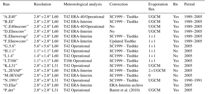
Fig. 1. Climatological convective updraft mass flux (kg m−2s−1) at 500 hPa averaged from (a) 40 reanalyses (1989–2001), (b) ERA-Interim reanalyses (1989–2005), (c) run “A E40” (1989–2005), and (d) run “B EI” (1989–2005).

4.1.1 Comparison of archived updraft convective mass flux with basic TOMCAT simulations

Figure 1 shows the climatological convective updraft mass flux at 500 hPa averaged from archived ERA-40 (1989–2001) and ERA-Interim (1989–2005) reanalyses as well as the basic TOMCAT simulations which are forced by ERA-40 (ECMWF operational analyses after 2001) and ERA-Interim reanalyses, respectively. The ECMWF archived mass fluxes show strong convection in the tropics especially around the South East Asia region. The ECMWF-Interim reanalyses have less convective updraft mass flux than ERA-40. The basic TOMCAT simulations forced by 40 and ERA-Interim both capture the climatological convection quite well and also reproduce the ERA-40 – ERA-Interim mass fluxes differences.

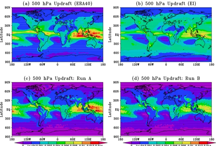
Figure 2 compares time series of the zonal mean updraft convective mass fluxes at 500 hPa from 40 and ERA-Interim reanalyses and TOMCAT runs “A E40” and “B EI”. At this altitude the model captures the annual cycle and latitudinal variation in the tropical convection. This figure again highlights that there are significant differences in the archived convective mass fluxes between the two ECMWF

datasets. The two basic model runs capture these differences but underestimate the archived mass flux values. Note the large change in modelled convection in run “A E40” in 2002 when ERA-40 analyses change to operational ones. Clearly, the performance of the model convection scheme changes strongly with the analyses used to force the model.

4.1.2 Impact of TOMCAT sensitivity experiments on updraft mass flux

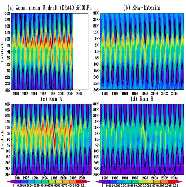
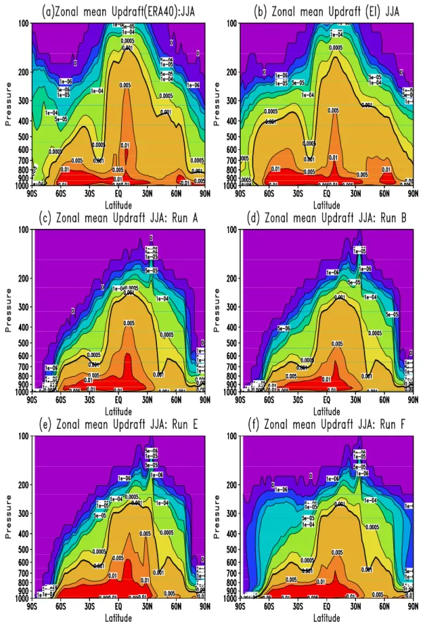
Figures 3 and 4 compare the JJA and DJF averaged zonal mean upward mass fluxes from archived 6-hourly ERA-40 and ERA-Interim reanalyses and calculated in selected TOMCAT experiments. The ECMWF archived mass fluxes show the expected behaviour of convection: there is max-imum updraft mass flux in the lower levels and larger val-ues in the tropical region. There is also stronger convec-tion in summer. Note that in the tropics these archived mass fluxes indicate that significant convective transport extends up to nearly ∼100 hPa, i.e. the tropopause region. The ERA-40 and ERA-Interim reanalyses show similar mass flux dis-tributions but there are differences in detail. For example, ERA-Interim gives smaller average convective transport in the tropics.

(8)

W. Feng et al.: Evaluation of cloud convection and tracer transport

15 Fig. 2. Time series of zonal mean monthly mean updraft convective

mass flux (kg m

−2

s

−1

) at 500 hPa from (a) ERA-40 reanalyses, (b)

ERA-Interim reanalyses, (c) Run “A E40” (forced by operational

winds from 2002 onwards), and (d) Run “B EI”. The bold contour

indicates 0.001 kg m

−2

s

−1

.

Fig. 2. Time series of zonal mean monthly mean updraft convective mass flux (kg m−2s−1) at 500 hPa from (a) ERA-40 reanalyses, (b) ERA-Interim reanalyses, (c) Run “A E40” (forced by operational winds from 2002 onwards), and (d) Run “B EI”. The bold contour indicates 0.001 kg m−2s−1.

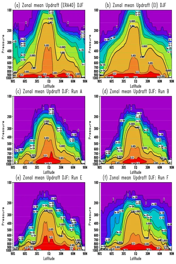
The diagnosed mean upward mass flux distributions from the four TOMCAT runs shown in Figs. 3 and 4 agree reason-ably well with the ECMWF reanalysis data below 200 hPa in the tropics. However, the most obvious disagreement is that the reanalyses show strong convective transport up to 100 hPa, i.e. well into the TTL, which is not captured by any of these TOMCAT runs (e.g. compare altitude of 0.001 kg m−2s−1 contour). The model also underestimates the convective mass flux in the mid-high latitudes.

When forced using different analyses the model does capture differences between ERA-40 and ERA-Interim archived mass fluxes. Run “A E40” (forced by ERA-40) gives stronger tropical convection below 200 hPa than run “B EI” (forced by ERA-Interim). This is due to differences in the large-scale wind, temperature and humidity fields

which drive the CTM. Run “E EInewevap” is the same as run “B EI” but uses higher horizontal surface evaporation fluxes. This data gives stronger convection below 400 hPa but there is little difference at higher altitudes in the tropics.

The basic TOMCAT convection scheme does not in-clude downdrafts and mid-level convection. We have tested the inclusion of these processes in model run “F EInewconv”. These make a significant difference to the calculated mass fluxes in mid latitudes (compare runs “E EInewevap” and “F EInewconv”) which improves agreement with the archived ECMWF fluxes. Note that there is less asymmetry of the weaker updraft contours between the northern and southern hemispheres in run “F EInewconv”. This is partly due to the criteria for the mid-level convection used in the Tiedkte (1989) scheme,

(9)

16 W. Feng et al.: Evaluation of cloud convection and tracer transport

Fig. 3. Zonal mean convective updraft mass flux (kg m

−2

s

−1

)

av-eraged for JJA from (a) 40 reanalyses (1989–2001), (b)

ERA-Interim reanalyses (1989–2005), (c) run “A E40” (1989–2005), (d)

run “B EI” (1989–2005), (e) run “E EInewevap” (1989–2005), and

(f) run “F EInewconv” (1989–2005). The bold contour indicates

0.001 kg m

−2

s

−1

.

Fig. 3. Zonal mean convective updraft mass flux (kg m−2s−1) averaged for JJA from (a) ERA-40 reanalyses (1989–2001), (b) ERA-Interim reanalyses (1989–2005), (c) run “A E40” (1989–2005), (d) run “B EI” (1989–2005), (e) run “E EInewevap” (1989–2005), and (f) run “F EInewconv” (1989–2005). The bold contour indicates 0.001 kg m−2s−1.

(10)

W. Feng et al.: Evaluation of cloud convection and tracer transport

17 Fig. 4. As Fig. 3, but for DJF.

Fig. 4. As Fig. 3, but for DJF.

(11)

18 W. Feng et al.: Evaluation of cloud convection and tracer transport

Fig. 5. Zonal mean convective updraft mass flux (kg m

−2

s

−1

) for

runs (a) “A E40”, (b) “B EI”, and (c) “N 1991” averaged from

27 December 1990–11 January 1991. The bold contour indicates

0.001 kg m

−2

s

−1

.

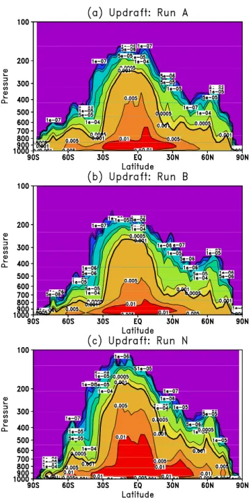
Fig. 5. Zonal mean convective updraft mass flux (kg m−2s−1) for runs (a) “A E40”, (b) “B EI”, and (c) “N 1991” averaged from 27 December 1990–11 January 1991. The bold contour indicates 0.001 kg m−2s−1.

which requires large-scale ascent and an environment rela-tive humidity of more than 90 %. However, on average run “F EInewconv” has less convective mass flux in the tropical low troposphere than “E EInewevap” and shows no improve-ment in the tropical UT.

Therefore, there is clearly a difference between diag-nosed convective mass fluxes in TOMCAT and the archived ECMWF reanalyses. The previous detailed analysis of the

TOMCAT convection scheme was performed by SC1999 where, based on short model runs, they concluded the model performed well. In order to compare our results with SC1999 we performed a run with the current version of TOM-CAT using the 1990/91 L31 operational ECMWF winds used by SC1999. Figure 5 compares results from this run “N 1991” with the two runs of the same model version which use the reanalysis data (runs “A E40” and “B EI”) averaged over the same period. The tropical convective mass fluxes are larger in the mid troposphere in run “N 1991” and ex-tend slightly higher. Therefore, results of the CTM convec-tion scheme do vary with different forcing datasets and older operational winds appear to give stronger tropical convection than the ERA-40 reanalyses. This illustrates possible dangers of comparing results from different experiments of the same CTM or of using results from an evaluation of the CTM dur-ing one period to explain results durdur-ing another. However, despite the slightly stronger convection in run “N 1991”, again the diagnosed convection does not extend as high in the tropics as indicated by the ECMWF reanalysis data.

The TOMCAT results presented so far have used a hori-zontal model resolution of 2.8◦×2.8◦and T42 (re)analyses. The resolution of both the model and the winds used to force it might be expected to impact on the diagnosed convection in the CTM; higher resolution might trigger more convective events.

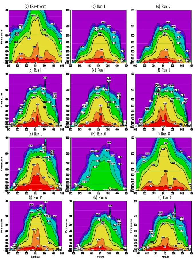
Figure 6 shows results from model sensitivity runs which investigate the effect of resolution in both the CTM and the forcing meteorology. On degrading the resolu-tion of the model and forcing analyses from 2.8◦×2.8◦ (run “E EInewevap”) to 5.6◦_×_5.6◦ _{(run “G 5.6”), the}

CTM produces less convective transport. Note that run “E EInewevap” uses ERA-Interim reanalyses while the oth-ers use operational forcing files. However, the change is not large compared to model versus archived mass flux dif-ferences. Similarly, on increasing the model resolution to 1.4◦×1.4◦ (run “I 1.4”) and 1.1◦×1.1◦ (run “H 1.1”), but with T42 analyses, although the diagnosed mass fluxes are larger, the calculated convection is similar. Finally, for the high resolution model (1.1◦×1.1◦) increasing the forcing analyses from T42 to T106 (runs “J T106” versus “H 1.1”) there is a further small increase in convective mass fluxes. Overall, however, the impact of large changes in resolution are small and do not really improve on the most significant discrepancies with the archived mass fluxes in the tropical upper troposphere and at high latitudes.

Figure 6 also shows results from runs “L 2EVAP” and “M 0EVAP” which investigate the sensitivity of the diag-nosed convection to large changes in the surface evaporation flux. These changes to the evaporation flux have large im-pacts on the modelled convection in the lower troposphere and in the tropical mid-troposphere, i.e. shallow convec-tion. However, even the extreme case of doubling the surface evaporation flux does not significantly change the modelled convective transport to the tropical UT.

(12)

W. Feng et al.: Evaluation of cloud convection and tracer transport

19

Fig. 6. Zonal mean annual mean convective updraft mass flux

(kg m

−2

s

−1

) for 2005 for (a) ERA-Interim reanalyses (1

◦

×1

◦

grid), (b) run “E EInewevap”, (c) run “G 5.6”, (d) run “H 1.1”,

(e) run “I 1.4”, (f) run “J T106”, (g) run “L 2EVAP”, (h) run

“M 0EVAP”, (i) run “O EIar”, (j) run “P det”, (k) run “A E40”,

Fig. 6. Zonal mean annual mean convective updraft mass flux (kg m−2s−1) for 2005 for (a) ERA-Interim reanalyses (1◦×1◦grid), (b) run “E EInewevap”, (c) run “G 5.6”, (d) run “H 1.1”, (e) run “I 1.4”, (f) run “J T106”, (g) run “L 2EVAP”, (h) run “M 0EVAP”, (i) run “O EIar”, (j) run “P det”, (k) run “A E40”, and (l) run “K L31”. The bold contour indicates 0.001 kg m−2s−1.

(13)

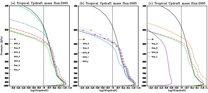
Fig. 7. Zonal mean annual mean tropical (25◦S–25◦N) updraft convective mass flux (kg m−2s−1) for 2005 from ERA-Interim reanalyses and (a) runs “A E40”, “B EI”, “E EInewevap”, “F EInewconv”, “K L31”, “N 1991” (December 1990 to January 1991), “O EIar”, “P det”,

(b) runs “E EInewevap”, “G 5.6”, “H 1.1”, “I 1.4”, “J T106”, and (c) runs “B EI”, “E EInewevap”, “L 2EVAP”, “M 0EVAP”.

Model run “P det” included changes to the TOMCAT convection scheme aimed at increasing tracer transport to the mid/upper tropical troposphere. In this run the annual mean, zonal mean convection does extend higher (e.g. the 0.001 kg m−2s−1 contour reaches 200 hPa) which is an im-provement over the basic model run. However, even this model run does not reproduce the convective mass fluxes above 200 hPa as archived in the ERA-Interim reanalyses.

Figure 6 also includes results from run “O EIar” in which TOMCAT was modified to read in the archived convective mass fluxes. In this run, as expected, the model convection agrees with the ERA-Interim reanalyses. The small differ-ence between panels (a) and (i) are due to the lower resolu-tion of the model run compared to the archived data.

Finally, Fig. 6 includes results from runs “P det”, “A E40” and “K L31” which used the same operational anal-yses for 2005. Here runs “P det” and “K L31” have the same vertical resolution (L31) while run “A E40” has a higher vertical resolution (L60). Increasing the vertical res-olution in run “A E40” does not have a significant impact on convection. However, the increase in vertical resolution on going from ECMWF L31 to L60 is mainly in the strato-sphere and so would not be expected to impact greatly on convection.

Figure 7 summarises the comparison of the tropical an-nual mean (2005) convective mass fluxes from ERA-Interim and a range of TOMCAT runs. Panel (a) compares differ-ent versions of the model and forcing wind fields, panel (b) compares different model and wind resolutions and panel (c) compares the impact of different surface evaporation fluxes. Figure 7a shows that up to about 300 hPa the experiments with different model formulation are similar to the archived

ECMWF values. Interestingly, run “N 1991”, which used older ECMWF operational analyses from 1990/91, shows the largest modelled convective mass fluxes below 200 hPa in this panel. Above 300 hPa there is a sharp fall off in the mod-elled convection except for runs “N 1991”, “P det” and run “O EIar” which uses archived mass fluxes. The sharp fall in the modelled convection from runs “N 1991” and “P det” oc-curs at/above 200 hPa. Run “P det”, in which a lower en-trainment rate is used, has significant convective mass fluxes extending higher (i.e. 0.001 kg m−2_s−1 _{reaches 200 hPa)}

than the other runs which diagnose convection. However, this profile comparison confirms that run “P det” also fails to reproduce the archived convective mass fluxes between 200 and 100 hPa. Figure 7b confirms that changing the resolution of the model and the analyses used to force the model has lit-tle impact on the diagnosed convection in TOMCAT. Higher resolution does lead to slightly more convection but the dif-ference is not large. Note that the model version which used archived mass fluxes (i.e. as used in run “O EIar”) would show even less sensitivity to resolution. Figure 7c shows that large changes to the assumed surface evaporation fluxes do have a large impact on modelled convection in the lower and mid troposphere.

4.2 Cloud top height comparison

A critical property of a convective parameterisation is the ability to accurately diagnose from the grid-scale forcing the depth to which convection occurs (e.g., Mahowald et al., 1995). As the formation of convective clouds depends on the occurrence of cumulus updrafts, observed cloud top height in convective regions can be used as a measure of the depth of convection.

(14)

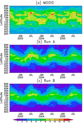
Fig. 8. Time series of monthly mean cloud top height (km) from (a)

MODIS (b) run “A E40”, and (c) run “B EI”.Fig. 8. Time series of monthly mean cloud top height (km) from (a)MODIS (b) run “A E40”, and (c) run “B EI”.

Figure 8 compares the observed cloud top height from MODIS for 2002–2005 with TOMCAT runs “A E40” and “B EI”. These model runs are representative of the basic TOMCAT runs which diagnose convection. The observa-tions show all observed clouds while the model results only show convective clouds. The model runs “A E40” and “B EI” capture the observed annual cycle of tropical (con-vective) clouds with the strongest convection occurring in the summer hemisphere. The modelled average tropical cloud top height peaks at about 10 km in the northern summer and about 8 km in the southern summer. This underestimates the observations which show mean cloud top heights up to 12– 13 km in both summer hemispheres.

Figure 9 shows a further comparison between MODIS and runs “A E40”, “B EI”, “K L31” and “P det”. For this figure, the maximum daily cloud top height in the tropics (30◦S– 30◦N) was found and then averaged into a monthly value. The highest monthly mean maximum cloud top heights oc-cur in the northern summer and are up to 15 km. In gen-eral TOMCAT underestimates the observed average maxi-mum cloud top height and in particular these large values

Fig. 9. Time series of monthly mean maximum daily cloud top height (km) for 2002–2005 averaged between 30◦S–30◦N from MODIS and model runs “A E40”, “B EI”, “K L31” and “P det”.

Fig. 9. Time series of monthly mean maximum daily cloud top

height (km) for 2002–2005 averaged between 30◦S–30◦N from MODIS and model runs “A E40”, “B EI”, “K L31” and “P det”.

around July. Run “K L31”, which has a lower vertical reso-lution than run “A E40”, generally shows a lower cloud top height. For this version of the model, modifications to the en-trainment/detrainment rates in run “P det” increase the cloud top height by up to 2 km. However, the model still underes-timates the highest observed cloud top heights.

Overall, Figs. 8 and 9 confirm that the model underesti-mates the vertical extent of tropical convection but the dis-crepancy of a few km in mean cloud top height does not ap-pear as large as the differences in the profile of the convective mass fluxes.

4.3 Convective precipitation

Surface rain rate is an important parameter in meteorology and is also important for the washout of some chemically ac-tive species. As precipitation rates are measured and archived by NWP reanalyses, they provide another meteorological comparison to test the overall performance of the CTM con-vection schemes. Column integrated precipitation will not be sensitive to key issues such as extent of convection in the tropical UT, but nevertheless will provide some information on the overall fidelity of the schemes used. Moreover, the wet deposition is also a key process for some trace gases and aerosols in the troposphere. Therefore, a discussion of con-vective precipitation will provide some useful information especially for the CTM modellers who are using the different ECMWF analyses.

Figure 10 shows zonal mean precipitation rates from observations (GPI and CMAP), meteorological reanalyses (ERA-40 and ERA-Interim) and model runs “A E40” and “B EI” from 1989 to 2005. The much larger precipitation rates in ERA-40 compared to ERA-Interim and the observa-tions can clearly be seen. The model captures the seasonal variation in precipitation. In the tropics, run “A E40”, forced by ERA-40 reanalyses, produces stronger precipitation than

(15)

W. Feng et al.: Evaluation of cloud convection and tracer transport

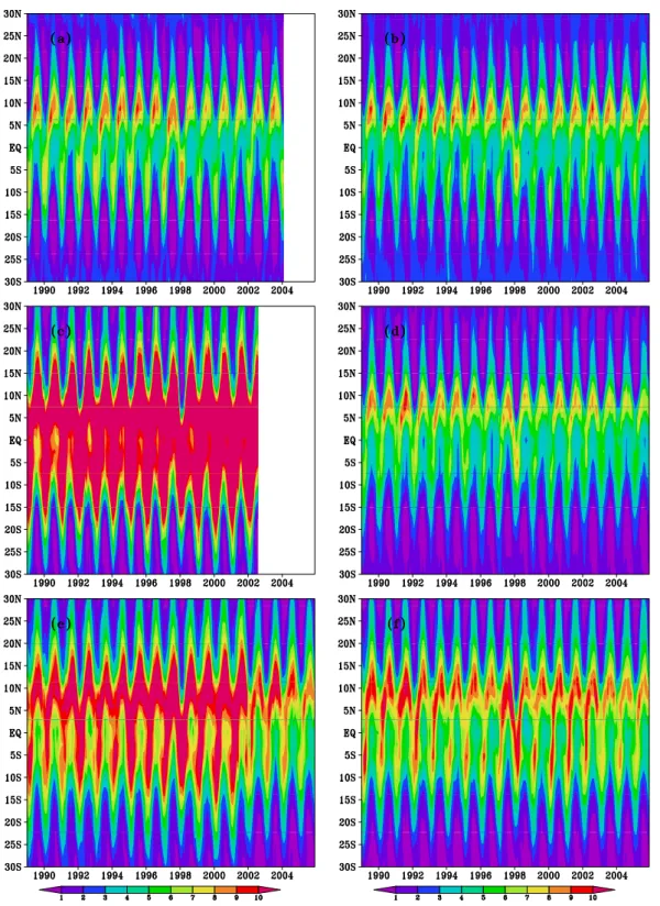
23 Fig. 10. Zonal mean convective precipitation (mm/day) from (a)

GPI data, (b) CMAP data, (c) ERA-40 reanalyses, (d) ERA-Interim

reanalyses, (e) run “A E40”, and (f) run “B EI”.

Fig. 10. Zonal mean convective precipitation (mm/day) from (a) GPI data, (b) CMAP data, (c) ERA-40 reanalyses, (d) ERA-Interim

reanalyses, (e) run “A E40”, and (f) run “B EI”.

run “B EI” which was forced by ERA-Interim, but both runs significantly underestimate precipitation in the extra-tropics. However, run “B EI” overestimates the peak mean values in the tropics compared to the observations and ERA-Interim,

while run “A E40” still underestimates the very large values of ERA-40. Further comparisons of precipitation rates for January and and July 2005 are shown in Fig. 11. This shows that the model generally captures the latitudinal variation of

(16)

Fig. 11. Zonal mean convective precipitation (mm/day) from

CMAP data, ERA-Interim reanalyses and model runs “A E40”, “B EI”, “K L31”, “P det” and “E EInewevap” for (a) January 2005, and (b) July 2005.

Fig. 11. Zonal mean convective precipitation (mm/day) from CMAP data, ERA-Interim reanalyses and model runs “A E40”, “B EI”, “K L31”, “P det” and “E EInewevap” for (a) January 2005, and (b) July 2005.

the observed/ERA-Interim precipitation but there are large differences between the experiments. Runs “A E40” and “B EI” slightly overestimate the observations in the tropics. Runs “K L31” and “P det” both use a lower vertical resolu-tion. Run “K L31” overestimates the observed precipitation rates in the tropics while run “P det”, which uses ISCCP data to specify the fraction of saturated water in each grid box, gives much better agreement. The model still underestimates the precipitation at latitudes higher than 30◦, though there is some improvement near 35◦–40◦using the updated Tiedkte convection scheme (Run “F EInewconv”).

4.4 Radon tracers

In this section we use observations of radon to investigate the accuracy of different convective treatments in the CTM. A number of the model runs include radon as a tracer us-ing a typical source distribution. Figure 12 compares how

modelled radon from selected runs compares with observa-tions at a range of surface sites. Generally, the model re-produces the observed magnitude of radon, showing that the assumed radon emissions produce realistic surface distribu-tions. TOMCAT gives a much better simulation of 222Rn for the oceanic sites (e.g., Amsterdam Island and Bermuda) since these sites are mainly affected by large-scale trans-port (see Zhang et al., 2008). However, the largest discrep-ancy occurs at the continental European station of Hohen-peissenberg where the model overestimates the surface ob-servations by up to a factor of 2. Zhang et al. (2008) pointed out that this is a challenging site for GCMs to simulate be-cause of the orography. This is also the case for CTMs like TOMCAT. There are various possible reasons for this over-estimation. Zhang et al. (2008) mentioned two main rea-sons from their GCM simulations: (1) The observed surface

222_{Rn depends strongly on the boundary layer. (2) The}

hori-zontal resolution in their GCM was coarse (∼300 km) which is similar to the experiments “A E40” and “B EI”. Another possible reason is that the222Rn flux we used in the model from Jacob et al. (1997) may overestimate the local emis-sions. For example, Conen and Robertson (2002) reported that the direct of222Rn flux measurement at this site is 0.75– 0.88 atoms cm−2s−1, while Zegvary et al. (2009) also re-ported even lower radon flux in Europe.

There are limited 222Rn vertical profiles from measure-ments. The climatological mid-latitude222Rn vertical pro-files from Liu et al. (1984) have been widely used for the evaluation of the tracer transport in global models (e.g., Stevenson et al., 1998; Zhang et al., 2008). The win-ter/summer 222Rn observations were obtained from indi-vidual aircraft measurements at different continental loca-tions from 1952 to 1972 (i.e., seven profiles for the winter and twenty three profiles for the summer). Figure 13a and b compare observed and modelled mean profiles of radon over Northern Hemisphere land areas for summer (JJA) and winter (DJF). Here we averaged the modelled 222Rn out-put between 30◦–60◦N among the land regions based on the land-sea mask information since there is limited infor-mation about the exact location and local time in the obser-vation profiles. The obserobser-vations show stronger lifting of radon (i.e. large concentrations around 10 km) in the sum-mer compared to the winter. The model runs which include convection agree reasonably well with the summer observa-tions. Runs “C E40noconv” and “D EInoconv”, which do not include convection more clearly underestimate the ob-servations, as expected. The stronger convective transport to higher altitudes in run “O EIar” appears to cause the model overestimation at the highest level (11 km). How-ever, the data does not extend to higher altitudes where the model-model differences are more prominent. In winter all the model runs show weaker convection and agree with the profile shape above 5 km, though none of the runs captures the observed C-shape profile at this latitude. Figure 13c and d show the absolute differences of radon between runs

(17)

W. Feng et al.: Evaluation of cloud convection and tracer transport

25 Fig. 12. Comparison of observed surface radon concentrations

(mBq/m

3

STP) with model runs “A E40” and “B EI” at (a)

Amster-dam Island (37.5

◦

S, 77.3

◦

E), (b) Bermuda (32.2

◦

N, 295.6

◦

E). (c)

Cape Grim (40.4

◦

S, 144.4

◦

E), (d) Par`a, Brazil (2.5

◦

S, 305

◦

E),

and (e) Hohenpeissenberg (47.5

◦

N, 11

◦

E). Note different x axis

and y axis scales.

Fig. 12. Comparison of observed surface radon concentrations (mBq/m3 STP) with model runs “A E40” and “B EI” at (a) Amsterdam Island (37.5◦S, 77.3◦E), (b) Bermuda (32.2◦N, 295.6◦E). (c) Cape Grim (40.4◦S, 144.4◦E), (d) Par`a, Brazil (2.5◦S, 305◦E), and (e) Hohenpeissenberg (47.5◦N, 11◦E). Note different x-axis and y-axis scales.

“A E40”-“B EI”, “D EInoconv”-“B EI”, “C E40noconv”-“A E40”, and “F EInewconv”-“E EInewevap” for summer and winter, respectively. The model forced by ERA-40 gives

slightly larger modelled radon tracer in the middle and up-per troposphere than when forced by ECMWF-Interim re-analyses. The difference between runs “C E40noconv” and

(18)

26 W. Feng et al.: Evaluation of cloud convection and tracer transport

Fig. 13. Comparison of observed radon profiles (mBq/m

3 STP)

averaged between 30

◦

N and 60

◦

N over land for (a) summer

(JJA) and (b) winter (DJF) with model runs “A E40”, “B EI”,

“C E40noconv”, “D EInoconv”, “E EInewevap”, “F EInewconv”,

“O EIar” and “P det”.

Panels (c) and (d) show the

dif-ferences between runs “A E40”-“B EI”, “D EInoconv”-“B EI”,

“C E40noconv”-“A E40”, and “F EInewconv”-“E EInewevap” for

summer and winter, respectively.

Fig. 13. Comparison of observed radon profiles (mBq/m3 STP) averaged between 30◦N and 60◦N over land for (a) summer (JJA) and (b) winter (DJF) with model runs “A E40”, “B EI”, “C E40noconv”, “D EInoconv”, “E EInewevap”, “F EInewconv”, “O EIar” and “P det”. Panels (c) and (d) show the differences between runs “A E40”-“B EI”, “D EInoconv”-“B EI”, “C E40noconv”-“A E40”, and “F EInewconv”-“E EInewevap” for summer and winter, respectively.

“A E40”, runs “D EInoconv” and “B EI”emphasise the ef-fect of convection in the modelled tracers in summer and winter. Obviously, the convection is very significant in sum-mer but small in winter for the northern hemisphere mid-latitudes as expected.

Figure 14 is a further comparison of radon profiles with campaign data from Moffett Field in June 1994 (Kritz et al., 1998) and the North Atlantic Regional Experiment (NARE) in August 1993 (Zaucker et al., 1996). The Moffett Field observations show large day-to-day variability in the profiles during the campaign. The observations from NARE do not extend above 6 km but show the modelled radon mixing

ra-tios in the lower atmosphere are reasonable. As model run “O EIar” does not cover the year of the observations results from runs “A E40” and “B EI” are plotted for both the obser-vation period and for 2005 to show the impact of interannual variability. Run “O EIar” produces higher radon values in the mid and upper troposphere than the other 2005 runs, al-though the model output for 1994 from runs “A E40” and “B EI” are larger above 11 km.

There have been extensive studies of the impact of reso-lution on the fidelity of model simulations (e.g., Phillips et al., 1995; Brankovic and Gregory, 2001; Lorant and Royer, 2001; Pope and Stratton, 2002; Rind et al., 2007; Wild, 2007;

(19)

W. Feng et al.: Evaluation of cloud convection and tracer transport

27 Fig. 14.

Comparison of observed radon profiles (mBq/m

3 STP) at (a) Moffett Field in June 1994 and (b) NARE

cam-paign in August 1993 with results from model runs “A E40”,

“B EI”, “C E40noconv”,

“D EInoconv”,

“E EInewevap”,

“F EInewconv” and “O EIar”. Panels (c) and (d) show the

same two campaigns as (a) and (b), respectively, along with model

runs “A E40” and “B EI” but also include results from model runs

“A E40”, “B EI”, “O EIar” and “P det” sampled for 2005.

Fig. 14. Comparison of observed radon profiles (mBq m−3STP) at (a) Moffett Field in June 1994 and (b) NARE campaign in August 1993 with results from model runs “A E40”, “B EI”, “C E40noconv”, “D EInoconv”, “E EInewevap”, “F EInewconv” and “O EIar”. Panels (c) and (d) show the same two campaigns as (a) and (b), respectively, along with model runs “A E40” and “B EI” but also include results from model runs “A E40”, “B EI”, “O EIar” and “P det” sampled for 2005.

Patra et al., 2008). They have shown that model resolution can play an important role in the simulation quality.

Clearly, the model has stronger vertical tracer transport at higher horizontal resolution. We have already shown that the diagnosed convection between these runs does not vary greatly, though it is stronger at higher resolution, and the large-scale winds are the same. An additional factor which leads to larger transport of radon at higher resolution is the ability of the model to resolve stronger spatial gradients in the tracer fields, and maintain larger local values. It should be noted that the vertical transport is not the only factor that

affects the radon profile. Horizontal mixing, particularly near coastal or snow covered areas may play a role, as there are strong spatial gradients in radon emissions here.

5 Discussion

The results presented here show a wide range in performance of the convection scheme in different CTM simulations. In particular, the comparison of the convective mass fluxes be-tween the runs which diagnose convection and that which

(20)

W. Feng et al.: Evaluation of cloud convection and tracer transport 5801 reads in the archived values will explain a large part of the

CTM differences seen in Hoyle et al. (2010). The use of convective mass fluxes from the same NWP system which produced the large-scale analyses appears to be more self-consistent than diagnosing them within the CTM with a dif-ferent code. However, this does not necessarily mean that the archived convective mass fluxes will directly lead to more re-alistic modelled tracer distributions.

In a recent study, Hossaini et al. (2010) used the TOM-CAT/SLIMCAT CTM to investigate the transport of the short-lived species CHBr3 (lifetime about 30 days) and

CH2Br2(lifetime about 6 months) to and through the TTL.

The version of TOMCAT used was the same as run “A E40” in this study, i.e. the default model but with 2007 winds. When comparing with aircraft campaign data, Hos-saini et al. (2010) showed that the p-level TOMCAT model tended to overestimate the abundance of these species in the TTL, suggesting that modelled vertical transport may be too rapid. In this study we show that run “A E40” produces con-vection which is less intense than other simulations, notably runs “O EIar” and “P det”. The implication here, therefore, is that stronger convection in TOMCAT would degrade the comparison of these short-lived tracers in the upper tropo-sphere. Hossaini et al. (2010) argued that the θ -level model (SLIMCAT) gave a more realistic tracer profile in the TTL due to slower large-scale advection. It is possible that a too strong large-scale advective transport overcompensated for an underestimate in convection.

Hossaini et al. (2010) also looked at the effect of convec-tion on CHBr3and CH2Br2by performing runs with this

pro-cess switched off. For these species, even without modelled convection (though still with mixing out of the PBL), there was still significant transport to the TTL. Of course, the ef-fect would have been more marked in a version of TOM-CAT with stronger convection (e.g. model version used in runs “O EIar” or “P det” as opposed to “A E40”) and for tracers with even shorter lifetimes. Lawrence and Salzmann (2008) raised questions about how results from experiments such as this should be interpreted. They argued that the ef-fects of convection cannot be removed by simply turning off the parameterisation in a CTM. They suggest that there is large overlap between the convective and large-scale trans-port, i.e. the resolved winds used in the CTM dynamics al-ready contain information about the convection.

6 Conclusions

We have used the TOMCAT 3-D off-line chemical transport model to investigate issues related to the treatment of vective tracer transport. The basic model diagnoses con-vection from the specified large-scale meteorological fields using a version of the Tiedtke scheme. For this work the Tiedtke scheme in the model has been updated to include mi-dlevel convection along with a new option to specify

convec-tion from archived convective mass fluxes. These archived mass fluxes provide a reference for the convection calculated within the CTM.

In general the model versions which diagnose convection underestimate the convective mass fluxes compared to the ECMWF archived values. The inclusion of midlevel con-vection in the updated TOMCAT model improves compar-isons at mid-high latitudes in the mid troposphere but there is still a significant disagreement in the latitudinal distri-bution (i.e., the modelled mass fluxes and precipitation are too low at mid-high latitudes). However, the most signifi-cant disagreement concerns the vertical extent of convection. The archived mass fluxes show significant tracer transport to about 100 hPa in the tropics while the diagnosed fluxes ex-tend to only around 200 hPa.

A range of model experiments have been performed with the version of the model which diagnoses convection. With the identical model code, there can be relatively large dif-ferences in diagnosed convection with different versions of ECMWF datasets. This needs to be borne in mind when comparing CTM results from different studies or when us-ing earlier evaluation of CTM convection to interpret recent results. The resolution of the CTM did not make a great dif-ference to the extent of diagnosed convective mass fluxes. The archived mass fluxes show strong convection transport up to 100 hPa, but none of the model experiments using the convection scheme are able to capture this though the model run using the old operational analyses has higher convective updraft mass fluxes. GCMs using different cumulus convec-tion schemes are also not able to reproduce this well (e.g., Tost et al., 2010). This is a challenge for CTMs/GCMs. At higher resolution there was more convective tracer trans-port. Changes to parameters in the Tiedtke scheme (en-trainment/detrainment rates) could be used to increase the extent of convective transport, but that may affect the pre-cipitation diurnal cycle as well as the mean and variability of the simulated precipitation as mentioned by Bechtold et al. (2004). Moreover, it is not clear if the changes in the en-trainment/detrainment rates would be altered by changes in the PBL parameterisation, the closure assumptions in the cu-mulus parameterisation and other model physical processes (Wang et al., 2007). Changes to the modelled surface evap-oration fluxes only impact shallow convective mass fluxes in TOMCAT.

The radon tracer has been included in the model runs. The limited profile observations available do not really discrim-inate between the different model versions. Clearly, some treatment of model convection in this paper improves agree-ment with observations. Despite relatively small changes in convective mass fluxes with resolution, higher model resolu-tion did result in high radon mixing ratios being transported to the mid troposphere. However, variability in the observa-tions means that both the diagnosed convection and using the archived convection agree with the data which extends up to 10 km in middle latitudes.

(21)

5802 W. Feng et al.: Evaluation of cloud convection and tracer transport While the use of archived mass fluxes would appear to be

an improvement for the CTM, and provide a model which is consistent with the forcing ECMWF meteorology, the sig-nificant transport to the tropical UT produced in this model needs to be tested. Observations of short-lived species in the tropical UT will be used for this in a future study extend-ing on the work of Hossaini et al. (2010) and Aschmann et al. (2009).

Acknowledgements. This work was supported by the European

Union SCOUT-O3 project and by NERC (NCEO and NCAS). The ECMWF analyses were obtained via the British Atmospheric Data Centre. We would like to thank three reviewers for their time and valuable suggestions which improved the quality of this paper. Edited by: P. Haynes

References

Arakawa, A.: Closure assumptions in the cumulus parameterization problem, in: The Representation of Cumulus Convection in Nu-merical Models, edited by: Emanuel, K. A. and Raymo nd, D. J., Amer. Meteor. Soc., Boston, USA, 1–15, 1993.

Arkin, P. A. and Meisner, B. N.: The relationship between large-scale convective rainfall and cold cloud over the Western Hemi-sphere during 1982–1984, Mon. Weather Rev., 115, 51–74, 1987. Aschmann, J., Sinnhuber, B.-M., Atlas, E. L., and Schauffler, S. M.: Modeling the transport of very short-lived substances into the tropical upper troposphere and lower stratosphere, Atmos. Chem. Phys., 9, 9237–9247, doi:10.5194/acp-9-9237-2009, 2009. Barret, B., Williams, J. E., Bouarar, I., Yang, X., Josse, B.,

Law, K., Pham, M., Le Flochmo¨en, E., Liousse, C., Peuch, V. H., Carver, G. D., Pyle, J. A., Sauvage, B., van Velthoven, P., Schlager, H., Mari, C., and Cammas, J.-P.: Impact of West African Monsoon convective transport and lightning NOx

pro-duction upon the upper tropospheric composition: a multi-model study, Atmos. Chem. Phys., 10, 5719–5738, doi:10.5194/acp-10-5719-2010, 2010.

Bechtold, P., Bazile, E., Guichard, F., Mascart, P., and Richard, E.: A mass-flux convection scheme for regional and global model, Q. J. Roy. Meteor. Soc., 127, 869–886, 2001.

Bechtold, P., Chaboureau, J. P., Beljaars, A., Betts, A. K., K¨ohler, M., Miller, M., and Redelsperger, J. L.: The simulation of the diurnal cycle of convective precipitation over land in a global model, Q. J. Roy. Meteor. Soc., 130, 3119–3137, 2004. Berntsen, T., Fuglestvedt, J., Myhre, G., Stordal, F., and Berglen, T.:

Abatment of greenhouse gases: does location matter?, Climatic Change, 74, 377–411, doi:10.1007/s10584-006-0433-4, 2006. Brankovic, T. and Gregory, D.: Impact of horizontal resolution on

seasonal integrations, Clim. Dynam., 18, 123–143, 2001. Breider, T., Chipperfield, M. P., Richards, N. A. D., Carslaw, K. S.,

Mann, G. W., and Spracklen, D. V.: The impact of BrO on dimethylsulfide in the remote marine boundary layer, Geophys. Res. Lett., 37, L02807, doi:10.1029/2009GL040868, 2010. Chipperfield, M.: New version of the TOMCAT/SLIMCAT

off-line chemical transport model: intercomparison of stratospheric tracer experiments, Q. J. Roy. Meteor. Soc., 132, 1179–1203, doi:10.1256/qj.05.51, 2006.

Chipperfield, M. P.: Multiannual simulations with a three-dimensional chemical transport model, J. Geophys. Res., 104, 1781–1805, 1999.

Chipperfield, M. P., Cariolle, D., Simon, P., Ramaroson, R., and Lary, D. J.: A 3-dimensional modeling study of trace species in the Arctic lower stratosphere during winter 1989–1990, J. Geo-phys. Res., 98, 7199–7218, 1993.

Conen, F. and Robertson, L. B.: Latitudinal distribution of radon-222 flux from continents, Tellus B, 54, 127-133, 2002.

Emanuel, K. A.: Atmospheric Convection, Oxford Univ. Press, New York, 580 pp., 1994.

Hodzic, A., Vautard, R., Chepfer, H., Goloub, P., Menut, L., Chazette, P., Deuz´e, J. L., Apituley, A., and Couvert, P.: Evo-lution of aerosol optical thickness over Europe during the Au-gust 2003 heat wave as seen from CHIMERE model simula-tions and POLDER data, Atmos. Chem. Phys., 6, 1853–1864, doi:10.5194/acp-6-1853-2006, 2006.

Holtslag, A. A. M. and Boville, B.: Local versus nonlocal boundary layer diffusion in a global climate model, J. Climate, 6, 1825– 1842, 1993.

Hossaini, R., Chipperfield, M. P., Monge-Sanz, B. M., Richards, N. A. D., Atlas, E., and Blake, D. R.: Bromo-form and dibromomethane in the tropics: a 3-D model study of chemistry and transport, Atmos. Chem. Phys., 10, 719–735, doi:10.5194/acp-10-719-2010, 2010.

Hoyle, C. R., Mar´ecal, V., Russo, M. R., Arteta, J., Chemel, C., Chipperfield, M. P., D’Amato, F., Dessens, O., Feng, W., Har-ris, N. R. P., Hosking, J. S., Morgenstern, O., Peter, T., Pyle, J. A., Reddmann, T., Richards, N. A. D., Telford, P. J., Tian, W., Vi-ciani, S., Wild, O., Yang, X., and Zeng, G.: Tropical deep con-vection and its impact on composition in global and mesoscale models – Part 2: Tracer transport, Atmos. Chem. Phys. Discuss., 10, 20355–20404, doi:10.5194/acpd-10-20355-2010, 2010. Jacob, D. J. and Prather, M. J.: Radon-222 as a test of convective

transport in a general circulation model, Tellus B, 42, 118–134, 1990.

Jacob, D. J., Prather, M. J., Rasch, P. J., et al.: Evaluation and inter-comparison of global atmospheric transport models using222Rn and other short-lived tracers, J. Geophys. Res., 102, 5953–5970, 1997.

Josse, B., Simon, P., and Peuch, V. H.: Radon global simulations with the multiscale chemistry and transport model MOCAGE, Tellus B, 56, 339–356, 2004.

Kain, J. S., Baldwin, M. E., and Weiss, S. J.: Parameterized updraft mass flux as a predictor of convective intensity, Weather Fore-cast., 106, 106–116, 2002.

Kritz, M. A., Rosner, S. W., and Stockwell, D. Z.: Validation of an offline three-dimensional chemical transport model using ob-served radon profiles – 1. Observations, J. Geophys. Res., 103, 8425–8432, 1998.

Lawrence, M. G. and Salzmann, M.: On interpreting studies of tracer transport by deep cumulus convection and its effects on atmospheric chemistry, Atmos. Chem. Phys., 8, 6037–6050, doi:10.5194/acp-8-6037-2008, 2008.

Liu, S. C., McAfee, J. R., and Cicerone, R. J., Radon 222 and tropospheric vertical transport, J. Geophys. Res., 89, 7219–7292, doi:10.1029/JD089iD05p07291, 1984.

Lorant, V., and Royer, J. F., Sensitivity of equatorial convection to horizontal resolution in aquaplanet simulations with a