Retirement and Unexpected Health Shocks

(1)

HAL Id: halshs-01670486

https://halshs.archives-ouvertes.fr/halshs-01670486v3

Preprint submitted on 1 Feb 2019

HAL is a multi-disciplinary open access archive for the deposit and dissemination of sci-entific research documents, whether they are pub-lished or not. The documents may come from teaching and research institutions in France or abroad, or from public or private research centers.

L’archive ouverte pluridisciplinaire HAL, est destinée au dépôt et à la diffusion de documents scientifiques de niveau recherche, publiés ou non, émanant des établissements d’enseignement et de recherche français ou étrangers, des laboratoires publics ou privés.

Retirement and Unexpected Health Shocks

Bénédicte H. Apouey, Cahit Guven, Claudia Senik

To cite this version:

Bénédicte H. Apouey, Cahit Guven, Claudia Senik. Retirement and Unexpected Health Shocks. 2019. �halshs-01670486v3�

(2)

WORKING PAPER N° 2017 – 59

Retirement and Unexpected Health Shocks

Bénédicte H. Apouey Cahit Guven Claudia Senik

JEL Codes: I12, I31, J26

Keywords : Retirement; Health Shocks; Life Satisfaction; Australia; HILDA

PARIS

-

JOURDAN SCIENCES ECONOMIQUES 48, BD JOURDAN – E.N.S. – 75014 PARIS

TÉL. : 33(0) 1 80 52 16 00=

www.pse.ens.fr

CENTRE NATIONAL DE LA RECHERCHE SCIENTIFIQUE – ECOLE DES HAUTES ETUDES EN SCIENCES SOCIALES

ÉCOLE DES PONTS PARISTECH – ECOLE NORMALE SUPÉRIEURE

(3)

Retirement and Unexpected Health Shocks

January 2019

Bénédicte H. Apouey

Affiliation: Paris School of Economics - CNRS, Paris, France E-mail: benedicte.apouey@psemail.eu

Cahit Guven

Affiliation: Deakin University, Department of Economics, Australia E-mail: cahit.guven@deakin.edu.au

Claudia Senik

Affiliation: Sorbonne University and Paris School of Economics, Paris, France E-mail: senik@pse.ens.fr

Acknowledgements

This paper uses data from the Household, Income, and Labour Dynamics in Australia (HILDA) survey. The HILDA project was initiated and is funded by the Australian Government Department of Social Sciences (DSS) and is managed by the Melbourne Institute of Applied Economic and Social Research (Melbourne Institute). The findings and views reported in this paper, however, are those of the authors and should not be attributed to either DSS or the Melbourne Institute. We thank F. Bourguignon, R. P. Ellis, P.-Y. Geoffard, I. Jelovac, J.-F. Laslier, Q. Roquebert, and L. Rochaix for useful comments.

We thank CEPREMAP, the French National Research Agency, through the program “Investissements d’Avenir” (ANR-10-LABX-93-01) and the JPI MYBL framework (ANR-16-MYBL-0001-02), for financial support.

Ethics approval

Ethics approval is not required since we analyze secondary, existing, HILDA data. The HILDA project was initiated and is funded by the Australian Government Department of Social Sciences (DSS) and is managed by the Melbourne Institute of Applied Economic and Social Research (Melbourne Institute).

(4)

2

Retirement and Unexpected Health Shocks

January 2019

Abstract

Is retirement good for your health? We complement previous studies by exploring the effect of retirement on unexpected health evolution. Using panel data from the Household, Income and Labour Dynamics in Australia survey (2001-2014), we construct measures of the mismatch between individual expected and actual health evolution (hereafter “health shocks”). In our approach, reverse causation running from health shocks to retirement is highly unlikely, because we look at shocks that happen at least a few months after retirement, and those shocks are, by definition, unanticipated. We find that retirement decreases the probability of negative shocks (by approximately 16% to 24% for males and 14% to 23% for females) while increasing the likelihood of positive shocks (by 9% to 14% for males and 10% to 13% for females). This result is robust to the use of different lead-lag structures and of alternative measures of health change. Our findings are thus consistent with a positive impact of retirement on health. We conclude that increasing the official retirement age may postpone the beneficial effect of retirement on health.

Keywords: Retirement; Health Shocks; Life Satisfaction; Australia; HILDA

(5)

3 1. Introduction

Workers generally plan to retire as soon as they are entitled to receive full pension benefits. In some countries, they massively protest against any attempt to increase retirement age. Obviously, this behavior is based on the expectation that retirement will be a source of greater wellbeing. But is it actually the case? Or do individuals underestimate the risk of loss of purpose and lack of socialization that may come with retirement? Behavioral economics has forcefully illustrated the possibility of such incorrect expectations. In this paper, we contribute to this strand of research by estimating the effect of retirement on unexpected health evolution.

A substantial literature explores the impact of retirement on general, physical, and mental health, life satisfaction, and lifestyles. Retirement could make people happier and healthier, given the deleterious impact of fatigue on aging workers, not to mention the case of strenuous work. However, retirement may also have a detrimental effect on wellbeing because it increases social isolation for individuals for whom the workplace is an important context of socialization. Empirically, identifying the causal effect of retirement on health is not straightforward. Indeed, current and expected health status certainly influences the decision to retire, as shown by Siddiqui (1997), Dwyer and Mitchell (1999), McGarry (2004), Au et al. (2005), Cai and Kalb (2006), Disney et al. (2006), and Bengtsson and Nilsson (2018). Similarly, Böckerman and Ilmakunnas (2009) find that workers in poor health self-select into unemployment in Finland. Moreover, both retirement and health may depend on unobserved confounding factors, such as time preferences.

To account for endogeneity, previous studies generally use an instrumental variable (IV) method, taking advantage of reforms that raise the pension age. Papers employ data from the U.S. Health and Retirement Survey (HRS), the European Survey on Health, Ageing and Retirement in Europe (SHARE), the European Survey on Income and Living Conditions

(6)

4

(SILC), the Household, Income and Labour Dynamics in Australia (HILDA) survey, and other country-specific surveys. Surprisingly, although they often use the same data and methods, findings are somewhat contradictory.

Several papers document a negative impact of retirement on health outcomes. For instance, using the HRS, Dave et al. (2008) show that retirement leads to an increase in difficulties associated with mobility and daily activities and in illness conditions, and to a decline in mental health. The literature also indicates that retirement exerts a negative effect on body weight for men who retire from strenuous jobs -- but not for women and workers in sedentary jobs -- both in the U.S. (Goldman et al., 2008) and in Europe (Godard, 2016). Some papers focus on the effect of retirement on cognitive abilities. Bonsang et al. (2012) find that retirement has a negative impact on cognitive functioning, using the HRS. Their result is supported by Mazzonna and Peracchi (2012) who employ the SHARE data and show that cognitive abilities decline at a higher pace after retirement. However, it is challenged by Coe et al. (2012) who use the same HRS data. Finally, Behncke (2012) employ the English Longitudinal Study of Ageing (ELSA) and shows that retirement significantly increases the risk of being diagnosed with a chronic condition, such as a severe cardiovascular disease and cancer. It also has a detrimental impact on other risk factors (e.g. BMI, cholesterol, and blood pressure), while worsening self-assessed health (SAH).

However, another series of studies uncovers a positive impact of retirement -- or a negative effect of employment at older ages -- on wellbeing in different countries. Shai (2018) uses data from three Israeli sources and shows that employment at older ages (due to the increase in the mandatory retirement age for males in 2004) is detrimental to health, especially for less-educated workers. Similarly, using HILDA, Zhu (2016) finds that retirement has a positive impact on self-reported health and on physical and mental health. Retirement also increases regular physical activity and reduces smoking. Mavromaras et al. (2013) and Atalay and Barrett

(7)

5

(2014) come to similar conclusions using Australian data. Other authors provide similar evidence based on the HRS (Insler, 2014), SHARE (Coe and Zamarro, 2011), SILC (Hessel, 2016), and German panel data (Eibich, 2015). In the latter paper, the channel is the relief from work-related stress and strain and the increase in sleep duration and in physical activity. Hallberg et al. (2015) reach the same conclusion using a reform in the retirement age of military officers in Sweden. Finally, some papers release more ambiguous results. In particular, Johnston and Lee (2009) find a positive impact of retirement on mental health and a less clear effect on physical health. Moreover, De Grip et al. (2015) show that retirees face lower declines in cognitive flexibility, but lower-educated retirees face greater declines with respect to information processing speed, compared to those who remain employed, in the Netherlands.

Differences in findings between studies may be due to differences in econometric specifications, control variables, and countries of interest. Nishimura et al. (2018) argue that for the same data and country, contradictory findings can be largely explained by the use of different methods.

Although this literature leads to interesting results, the IV method has some limitations. Indeed, this approach estimates the effect of retirement for a very specific subpopulation -- the so-called compliers -- rather than for the entire population. While many workers will postpone retirement following a reform, some individuals will still retire earlier, to prioritize their health for instance. Because compliers may differ from the rest of the population, the estimated effect in the IV approach could be different from the average treatment effect. More importantly, reforms that postpone retirement put people in a situation where their expectations are not met and force them to change their plans. This may directly affect their wellbeing and health. In that case, the effect estimated using the IV method could be due to the unexpected nature of the reform, in addition to retirement status itself.

(8)

6

In this article, we complement the previous literature by employing a different strategy to explore the relationship between retirement and health. Specifically, we estimate the impact of retirement on unexpected health shocks. Like the IV method, our strategy addresses the problem of reverse causation, but in an original way. Reverse causality is highly unlikely in our setting because we look at shocks that happen at least a few months after retirement, and those shocks are, by definition, unanticipated.

Our data come from the HILDA panel survey. At each wave of the survey, respondents answer the Short Form 36 (SF-36) questions about their health. In particular, individuals are asked about their expected changes in health in the future. Moreover, they assess their health evolution over the past year (“reported health transition”). Respondents also answer each year a standard SAH question and a series of questions on physical and mental health. We use this information to compute the change in SAH and in mental and physical health over time, for each respondent. By combining information on prospective expectations with information on retrospective (reported or computed) health evolutions, we construct a series of measures of unexpected health shocks. We distinguish between positive and negative shocks. We then estimate the effect of labor market status on these positive and negative health shocks. Regressions are estimated using the entire sample of individuals aged 50-75, that contains all individuals who transition to retirement. Employing a lead-lag structure, we capture the impact of individual labor market status on health shocks that occur later. To account for unobserved heterogeneity, we exploit the longitudinal nature of the data and include individual fixed effects in our models. As mentioned earlier, several papers use the same HILDA survey to explore the effect of

(9)

7

retirement on health. However, they do not take advantage of information on health expectations.1

Our findings indicate that retirement decreases the likelihood of negative health shocks and increases the likelihood of positive shocks. For both genders, retirement comes with an unexpected improvement in general, physical, and mental health. For men, retirement increases the probability of a positive health shock up to 14%, depending on specifications; and for women, the effect reaches 13%. Our results are robust to the inclusion of controls for past health shocks and lagged health status. We check that reported health transitions are consistent with computed evolutions of other health measures. Finally, we find that health shocks are associated with life satisfaction: for both genders, unexpected positive health shocks go hand in hand with both a higher level of life satisfaction and a greater improvement in life satisfaction over time.

The paper proceeds as follows. Section 2 describes the HILDA data. Section 3 presents the empirical model and the estimation strategy. Section 4 contains our main findings while Section 5 presents some robustness checks and additional results. Section 6 contains some concluding remarks.

2. Data

The HILDA Survey

We use longitudinal data from the Household, Income and Labour Dynamics in Australia (HILDA) survey, waves 1 to 14, covering the 2001-2014 period. HILDA annually collects information on economic wellbeing, labor market status, and health status, for all adults (aged 15+). Our sample contains 51,000 observations, corresponding to 4,400 females and 4,800

1_{They also use a different definition of retirement. For instance, Zhu (2016) defines retirement as not being in the}

labor force, whereas we assume that a person is retired if she reports that she does not work and that she is completely retired.

(10)

8

males aged 50 to 75 between 2001 and 2014. We observe 737 transitions to retirement for men

and 933 for women.

The SF-36

We use information from the 36-item Short Form Health Survey (SF-36) to measure unexpected changes in health. The SF-36 is a patient-reporting outcome measure that quantifies health status. The survey contains 36 questions, which capture eight health concepts -- physical functioning (PF), role functioning/physical (RP), bodily pain (BP), general health perceptions (GH), vitality (VT), social role functioning (SF), mental health (MH), and role functioning/emotional (RE) -- as well as reported health transition (see below).

Health Expectations

To construct our variables of interest, we combine information on health expectations and on actual health evolution. The question capturing overall health expectations is the following: “How true of false is [each of] the following statement for you? I expect my health to get worse.” Respondents must select one of the following answers: “Definitely true,” “Mostly true,” “Don’t

know,” “Mostly false,” and “Definitely false” (the name of the variable is gh11c). We recode

the variable into three categories: True, Don’t know, and False. The question does not explicitly mention any time horizon.

Reported Health Transitions

We measure the actual evolution of individual health in several manners. First, we use the

following question on health transition from the SF-36: “Compared to one year ago, how would

you rate your health in general now?” The response categories are the following: “Much better

now than one year ago,” “Somewhat better than one year ago,” “About the same as one year

ago,” “Somewhat worse than one year ago,” and “Much worse than one year ago” (the name

(11)

9

Computed Evolution of SAH, Physical Health, and Mental Health

We also use the SF-36 to construct additional health evolution variables. We employ the following SAH question: “In general, would you say that your health is: Excellent, Very good,

Good, Fair, Poor?” We also use the 35 questions from the SF-36 and create a physical

component summary (PCS) and a mental component summary (MCS), which are summary measures that capture the two dimensions of the SF-36. For each individual, we then calculate the evolution of SAH, PCS, and MCS between t and T (T = t+1 or t+2) and create a series of health evolution variables that indicate whether the respondent’s health worsens, remains stable, or improves over time. We assume that PCS worsens between t and T if PCS in T is smaller than PCS in t minus one standard deviation; we consider that PCS remains the same if PCS in T is greater than PCS in t minus one standard deviation and smaller than PCS in t plus one standard deviation; and finally we assume that PCS increases if PCS in T is greater than PCS in t plus one standard deviation. We define deterioration, stability, and improvement in MCS in a similar way.

Unexpected Shocks

We create our shock variables by comparing expectations reported in t with actual evolutions. Actual evolutions are captured either by the “reported health transition” which is reported in t+1, or by the computed evolution of SAH, PCS, and MCS between t and T (Table 1).

[Insert Table 1 here]

Life Satisfaction

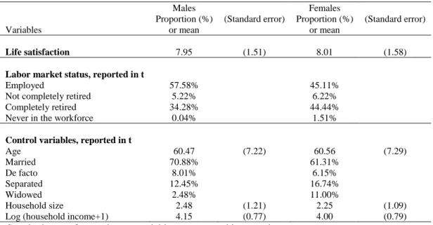
Life satisfaction is the answer to the question: “How satisfied are you with your life?” with a scale ranging from 0 (“Totally dissatisfied”) to 10 (“Totally satisfied”). In our regression sample, the average level of life satisfaction reaches 7.95 for males and 8.01 for females. This

(12)

10

question is routinely used in large surveys to measure subjective wellbeing, e.g. in the World Values Survey, the European Social Survey, the British ONS, the German SOEP, and Gallup and OECD surveys, for instance. In our analysis, we use two different life satisfaction outcomes: life satisfaction level (which is the direct answer to the question) and life satisfaction evolution. To capture evolution, we construct dummies capturing whether individual life satisfaction decreases, remains the same, or decreases between two consecutive years.

Retirement and Labor Market Status

Several definitions of retirement are employed in the literature. For instance, using the GSOEP, Eibich (2015) assumes that an individual is “retired” if she reports that she is retired and that she does not work, even part-time, while using HILDA, Zhu (2016) considers that a person is retired if she reports that she is not in the labor force. Here, we adopt a more restrictive definition and focus on “complete retirement.” Specifically, the data indicate whether individuals are employed, unemployed, or not in the labor force (NLF). In addition, individuals who are 45 years and above and who do not work are asked the following question: “Have you

retired (completely) from the workforce?” The response categories are the following: “Yes,”

“No,” and “Never in the workforce.” This question is asked in every wave except in 2003, 2004, 2007, and 2011. In order to avoid losing observations in 2003 and 2004, we assume that if an individual is completely retired in 2002 and in 2005, then she is also completely retired in 2003 and 2004. Similarly, we assume that if she is not completely retired in 2002 and 2005, then she is not completely retired in 2003 and 2004. We proceed in the exact same way for 2007 and 2011.

By combining the answers to these two questions, we create a categorical variable indicating whether the individual is (i) employed (reference category), (ii) unemployed or NLF and not completely retired, (iii) unemployed or NLF and completely retired, and (iv) unemployed or

(13)

11

NLF and never in the workforce. We are interested in the association between complete retirement and health shocks. In our regressions, “employed” serves as the reference category.

Descriptive Statistics

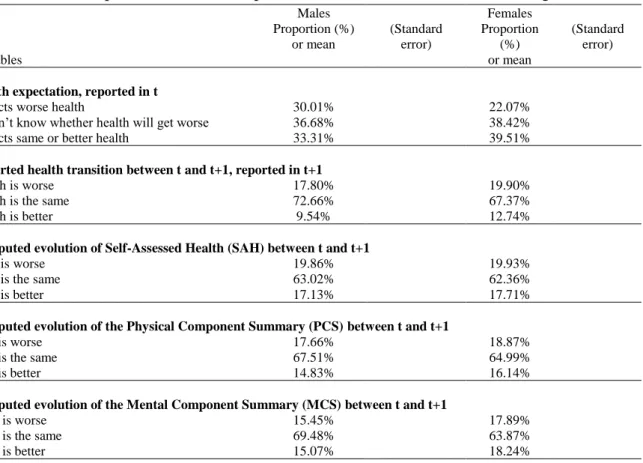
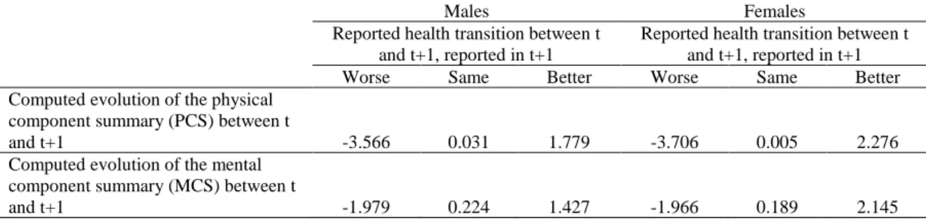
Table 2 provides summary statistics for the entire sample. Over one third of individuals do not have a precise idea of how their health will change in the future; about one quarter expect a worsening, and over one third expect an improvement or no change. Moreover, females are more optimistic than males. Regarding reported health evolution, a large majority (73%) of men acknowledge no change in their health, 10% report an improvement, and 18% a worsening. Women are less likely to report no change than men. The constructed measures of health evolution tell a similar, although slightly rosier, story. SAH declines for 20% of the sample, remains similar for about 63% of individuals, and improves for approximately 17% of the sample. Evolutions of PCS and MCS variables are of the same magnitudes. Note that reported health transitions are consistent with computed health evolutions: for instance, reporting worse health goes hand in hand with a decrease in the PCS and MCS scores (Table A1 in Appendix A).

The bottom of Table 2 provides descriptive statistics for shocks between t and t+1 (we do not report these for other shocks for space reasons). Concerning reported health transition, 9% of males experience a negative shock, while 24% experience a positive shock. For females, the proportions are 11% and 18%. Hence, females experience more negative shocks and less positive shocks than males.

(14)

12

Table 3 indicates that 58% of males and 45% of females are employed, while 34% of men and 44% of women are completely retired. 71% of males and 61% of females are married. The average age in the sample is 60 years for men and 61 years for women.

3. Empirical Model

To explore the potential effect of retirement on health shocks, we estimate the following model using OLS-Fixed Effects:

Yi,(t,T) = LMSi,t.β + Xi,t.δ + ρt + αi + εi,t,T with T = t+1 or t+2 (1)

Yi,(t,T) denotes health shocks experienced by individual i between t and T (with T = t+1 or t+2). These shocks are constructed using expectations reported in t and evolutions between t and T.

Moreover, LMSi,t represents measures of labor market status -- employed (reference category),

not completely retired, completely retired, and never in the workforce -- reported in t. Note that

β thus captures the effect of labor market status on shocks. Xi,t denotes the following control

variables: age, age square, marital status, family size, and the logarithm of household income.

In addition, ρt represents year dummies. Finally, αi captures individual fixed effects, that include

personal optimism or pessimism in particular.

Importantly, individuals who report that they are retired (on the day of the survey) in t have retired before the survey. In other words, information on their health expectations (reported in t) are collected after their transition to retirement. This minimizes the risk of reverse causation.

Given that we include individual fixed effects, the impact of “never in the workforce” should not be identified. However, a small fraction of respondents do not consistently report that they have never been in the workforce across survey years (measurement error).

(15)

13

We also explore the impact of labor market status reported in t on health shocks between t+1 and t+2. In that case, expectations are reported in t+1, and health evolutions capture changes

between t+1 and t+2.The model writes in the following way:

Yi,(t+1,t+2) = LMSi,t.β + Xi,t.δ + ρt + αi + εi,t,t+1,t+2 (2)

Labor market status is thus reported one year before expectations and two years before health evolutions. This makes reverse causation highly unlikely.

Given differences in labor market histories, models are estimated for females and males separately. In all specifications, we compute robust standard errors.

4. Main Results

We first discuss the effect of labor market status (in t) on health expectations (in t) and health evolutions (between t and T) separately. Results are shown in Table B1 in Appendix B. When they are retired, males are more likely to expect that their health will deteriorate than when they are employed (Panel A, column (1)). However, retirement decreases the likelihood of health deterioration (Panel F, column (1)), while increasing that of health improvement (Panel B, column (3)), for males. In particular, retirement increases the probability of health improvement by 2.5 percentage points (Panel B, column (3)).

For females, while retirement is not significantly correlated with expectations, it is negatively associated with health deterioration (Panels B to E, column (4)) and positively correlated with health improvement (Panels C, E, and F, column (6)).

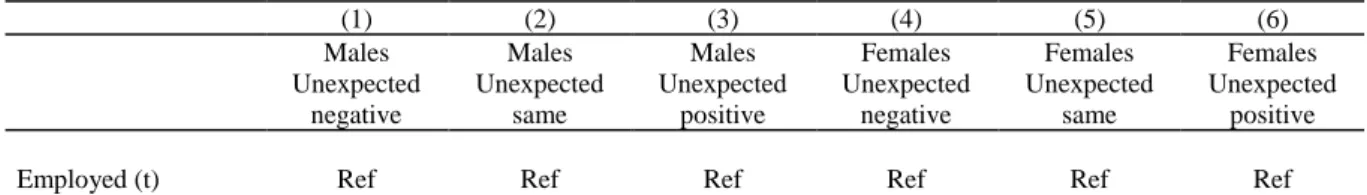
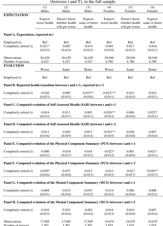
In Table 4, we present the effect of retirement (in t) on shocks (between t and T), estimated using Equation (1). In a nutshell, results indicate that retirement has a beneficial influence on health shocks for both genders. More precisely, for males, retirement decreases the likelihood of negative shocks (Panels A and B, column (1)) and increases that of positive shocks (Panels

(16)

14

A and D to G, column (3)). For instance, complete retirement decreases the probability of unexpected negative shocks by 2.0 percentage points (Panel A), i.e. 23.6% (since 8.6% of males experience a negative shock, as shown in Table 2). Retirement also increases the likelihood of unexpected positive shocks by 3.4 percentage points, i.e. 14.2% (Panel A). The magnitude of the effect of retirement on health shocks is relatively large: when the effect of retirement is significant, the decrease in negative shocks varies between 15.9% and 23.6%, while the increase in positive shocks varies between 9.1% and 14.2%.

Similarly, females are less likely to experience negative shocks (Panels A to D, column (4)) and more likely to experience positive shocks (Panels B and E, column (6)). For instance, retirement is accompanied by a 22.5% reduction in unexpected negative shocks for them (Panel A, column (4)).

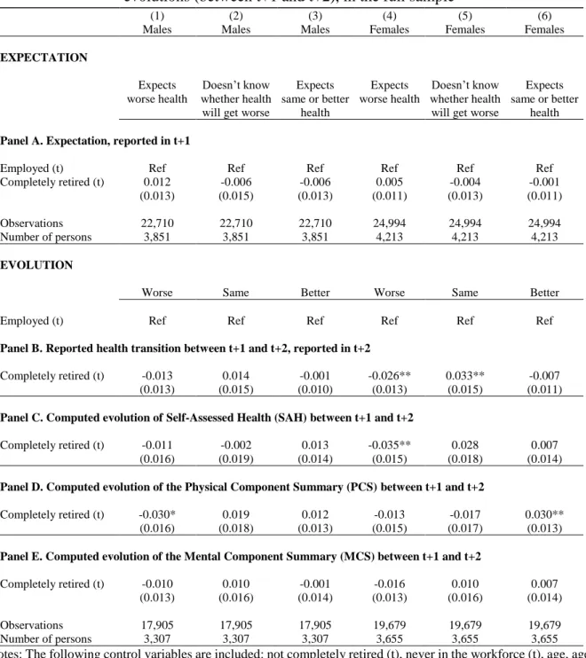
We now focus on shocks that happen between t+1 and t+2. Results are reported in Table 5. They support our previous findings on the beneficial impact of retirement on shocks: retirement has a negative impact on negative health shocks (for both genders) and a positive effect on positive shocks (for females). On a related matter, Table C1 in Appendix C shows that retirement is negatively associated with health degradation (for both genders) and is positively correlated with health improvement (for females) (between t+1 and t+2) but is not linked to expectations (reported in t+1).

A natural question is whether the effect of retirement depends on the type of occupation, and in particular whether it is different for blue-collar and white-collar workers. The impact could also depend on whether individuals have a partner, and whether this partner is herself retired or not.

(17)

15

As it turns out, although these characteristics are correlated with respondents’ health status, they are not associated with health shocks, i.e. with unexpected changes in health status. These results are not reported for space reasons.

5. Sensitivity Analysis and Additional Results

This section provides some robustness checks and additional results. Note that we do not systematically report the results for all shock measures for space reasons.

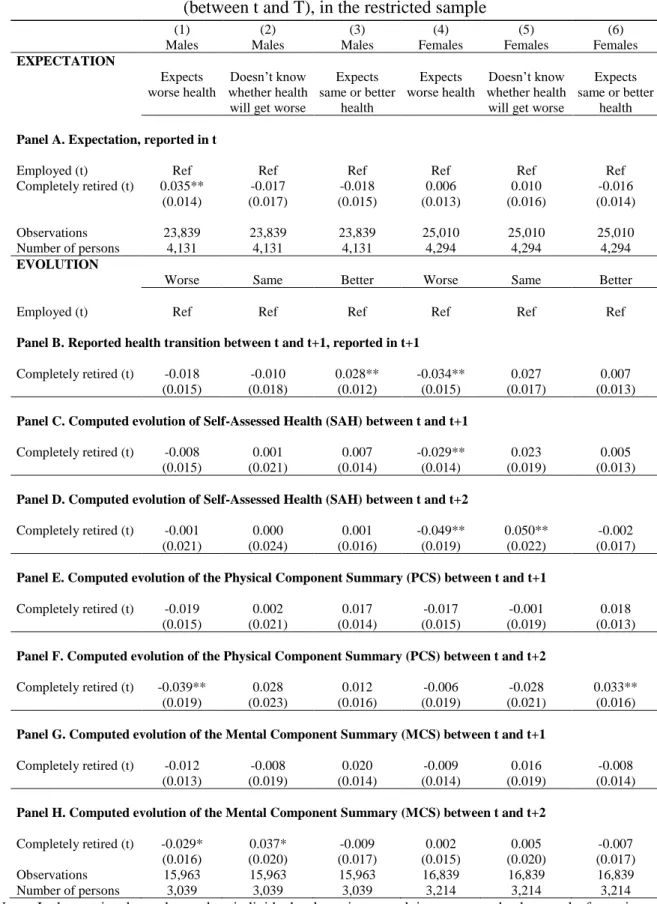
Restricted Sample

Approximately 700 individuals (300 males and 400 females) retire several times, or come back to the labor force after retirement. To check the robustness of our results, we create a restricted sample from which these individuals are excluded, and re-estimate Equation (1) using this smaller sample. Results regarding shocks are qualitatively similar, but coefficients are larger and more often significant (Tables D1 and D2 in Appendix D). Table D1 highlights that complete retirement is positively associated with expectations that health will worsen in the future, for males. Table D2 clearly shows the beneficial effect of retirement on health shocks for both females and males.

Shocks Between t-1 and t

We also re-estimate our main model measuring health shocks between t-1 and t (health shocks were previously measured between t and T or between t+1 and t+2). Labor market status is measured in t, like in our previous specifications. Expectations are now reported one year before, in t-1. Information on health transition is reported in t, and computed health evolution uses information on health status in t-1 and t.

Individuals who report that they are retired (on the day of the survey) in t have retired before the survey. Consequently, information on their health transition (reported in t) is collected after

(18)

16

their transition to retirement. Similarly, computed health evolution uses information on health status that is collected in t, i.e. after the retirement transition (and information collected in t-1, i.e. before retirement).

Results (Table E1 in Appendix E) are consistent with our previous findings. Retirement is systematically positively correlated with positive shocks for males. For women, retirement is associated with an increase in the probability of positive shocks when we use the SAH variable.

Additional Controls

We also re-estimate our models including additional control variables. First, past health shocks may have an impact on labor market status. To address this issue, we include lagged health shocks on the right-hand side of the models (Table F1 in Appendix F). We obtain consistent results: retirement is still negatively associated with negative health shocks (for both genders) and positively correlated with positive shocks (for males).

As documented in the previous literature, some people may retire because of poor health. To account for this, we control for lagged SAH (Table F2 in Appendix F). The results are robust to the inclusion of this additional control: for males, complete retirement is associated with positive health shocks, and for females, it is negatively correlated with negative shocks.

Attrition

Attrition may affect the representativeness of the sample and lead to biased estimates of the impact of retirement. To adjust for attrition, we re-estimate our models using longitudinal weights (Table G1 in Appendix G). Results are consistent with our previous findings.

(19)

17 Event studies

To illustrate our results on the effect of retirement, we try to display estimates of anticipation and adaptation to retirement in terms of health shocks (i.e. lags and leads in shocks). Because our results are generally not statistically significant, but provide suggestive evidence which is consistent with our main findings, we report them in Appendix H (Figure H1). We also explore lags and leads around the time of unemployment spells and other life events (see Figures H2 and H3 and related comments in Appendix H).

Health Shocks and Life Satisfaction

Finally, we study the link between health shocks and life satisfaction. The results are displayed in Appendix I. First, in Table I1, we regress life satisfaction levels (in t+1) on shocks (between t and t+1) and controls. Unsurprisingly, positive health shocks are associated with higher levels of life satisfaction than negative shocks. In Table I2, we regress dummies capturing a decrease, stability, or increase in life satisfaction (between t and t+1) on shocks (between t and t+1). Again, positive shocks go hand in hand with positive evolutions of life satisfaction. Hence, the positive health shocks that follow retirement are associated with consistent satisfaction outcomes.

Note that we do not claim any causality running in either direction. We simply show that health shocks and retirement are significantly associated, whether this means that health influences life satisfaction or the reverse.

6. Conclusion

This paper explores the impact of retirement on unexpected health changes, using longitudinal data on older Australians from the 2001-2014 HILDA panel survey. In our approach, health

(20)

18

shocks capture the difference between ex ante expected health status and ex post health evolution.

Evaluating the causal impact of retirement on health is not straightforward. Indeed, workers may retire because of ill health or disability, creating a reverse causation concern. To address this issue, social scientists usually exploit reforms that raise the retirement age and study the impact of additional years of activity on workers affected by the reform. However, this IV approach also has some limitations, because of non-compliance and because the reform may lead to frustration for affected workers. Moreover, the conclusions of these studies are somewhat contradictory: some point to the beneficial effect of retirement on health while others uncover a detrimental effect.

In our study, we complement the previous literature by evaluating the effect of retirement on unexpected health shocks. The risk of reverse causality running from shocks to retirement is highly unlikely, because health shocks are unexpected by definition, and because they are measured after the retirement transition. We find that retirement lowers the likelihood of negative shocks and increases that of positive shocks. The results are robust to the use of alternative definitions of health evolution. Moreover, effects are economically significant: in some specifications, the likelihood of negative shocks decreases by 24% after retirement. There is no evidence that the impact of retirement on shocks depend on occupation or marital status. Many developed countries have recently increased pension eligibility age. Our paper implies that even if they are necessary, such reforms may postpone the beneficial effects of retirement on health.

(21)

19 References

Atalay, K., & Barrett, G. F. (2014). The causal effect of retirement on health: New evidence from Australian pension reform. Economics Letters, 125(3), 392-395.

Au, D. W. H., Crossley, T. F., & Schellhorn, M. (2005). The effect of health changes and long‐ term health on the work activity of older Canadians. Health Economics, 14(10), 999-1018. Behncke, S. (2012). Does retirement trigger ill health? Health Economics, 21(3): 282-300. Bengtsson, T., & Nilsson, A. (2018). Smoking and early retirement due to chronic disability.

Economics & Human Biology, 29, 31-41.

Böckerman, P. & Ilmakunnas, P. (2009). Unemployment and self-assessed health: Evidence form panel data. Health Economics, 18(2): 161-179.

Bonsang, E., Adam, S., & Perelman, S. (2012). Does retirement affect cognitive functioning?

Journal of Health Economics, 31(3): 490-501.

Cai, L., & Kalb, G. (2006). Health status and labour force participation: Evidence from Australia. Health Economics, 15(3), 241-261.

Coe, N. B., von Gaudecker, H. M., Lindeboom, M., & Maurer, J. (2012). The effect of retirement on cognitive functioning. Health Economics, 21(8), 913-927.

Coe, N. B., & Zamarro, G. (2011). Retirement effects on health in Europe. Journal of Health

Economics. 30(1), 77-86.

Dave, D., Rashad, I., & Spasojevic, J. (2008). The effects of retirement on physical and mental health outcomes. Southern Economic Journal, 75(2): 497-523.

De Grip, A., Dupuy, A., Jolles, J., & Van Boxtel, M. (2015). Retirement and cognitive development in the Netherlands: Are the retired really inactive? Economics & Human Biology, 119, 157-169.

Disney, R., Emmerson, C., & Wakefield, M. (2006). Ill health and retirement in Britain: A panel data-based analysis. Journal of Health Economics, 25(4), 621-649.

Dwyer, D. S. & Mitchell, O. S. (1999). Health problems as determinants of retirement: Are self-rated measures endogenous? Journal of Health Economics, 18(2): 173-193.

Eibich, P. (2015). Understanding the effect of retirement on health: Mechanisms and heterogeneity. Journal of Health Economics, 43: 1-12.

Godard, M. (2016). Gaining weight through retirement? Results from the SHARE survey.

(22)

20

Goldman, D., Lakdawalla, D., & Zheng, Y. (2008). Retirement and weight, mimeo. Available at: http://www.aeaweb.org/assa/2009/retrieve.php?pdfid=219.

Hallberg, D., Johansson, P., & Josephson, M. (2015). Is an early retirement offer good for your health? Quasi-experimental evidence from the army. Journal of Health Economics, 44, 274-285.

Hessel, P. (2016). Does retirement (really) lead to worse health among European men and women across all educational levels? Social Science & Medicine, 151, 19-26.

Insler, M. (2014). The health consequences of retirement. Journal of Human Resources, 49(1), 195-233.

Johnston, D. W., & Lee, W. S. (2009). Retiring to the good life? The short-term effects of retirement on health. Economics Letters, 103(1), 8-11.

Mavromaras, K., Richardson, S., & Zhu, R. (2013). Age pension, age eligibility, retirement and health outcomes in Australia. National Institute of Labour Studies WP, (201).

Mazzonna, F. & Peracchi, F. (2012). Ageing, cognitive abilities and retirement. European

Economic Review, 56(4): 691-710.

McGarry, K. (2004). Health and retirement do changes in health affect retirement expectations?

Journal of Human Resources, 39(3), 624-648.

Nishimura, Y., Oikawa, M., & Motegi, H. (2018). What explains the difference in the effect of retirement on health? Evidence from global aging data. Journal of Economic Surveys, 32(3), 792-847.

Shai, O. (2018). Is retirement good for men’s health? Evidence using a change in the retirement age in Israel. Journal of Health Economics, 57, 15-30.

Siddiqui, S. (1997). The impact of health on retirement behaviour: Empirical evidence from West Germany. Health Economics, 6(4), 425-438.

Zhu, R. (2016). Retirement and its consequences for women’s health in Australia. Social

(23)

21 TABLES

Table 1. Construction of the shock variables when expectations are reported in t

Variable label Definition

Unexpected negative shock between t and T

Doesn’t know whether health will get worse (reported in t) & Health gets worse between t and T

Expects same or better health (reported in t) & Health gets worse between t and T

Unexpected same shock between t and T

Doesn’t know whether health will get worse (reported in t) & Health remains the same between t and T

Unexpected positive shock between t and T

Expects worse health (reported in t) & Health remains the same between t and T

Expects worse health (reported in t) & Health improves between t and T Doesn’t know whether health will get worse (reported in t) & Health improves between t and T

Expected negative change between t and T

Expects worse health (reported in t) & Health gets worse between t and T

Expects same or better health (reported in t) & Health remains the same between t and T Expects same or better health (reported in t) & Health improves between t and T

Notes: T = t+1 or t+2. The last two rows of the table contain ambiguous cases that combine anticipated and unanticipated changes.

(24)

22

Table 2. Descriptive statistics for expectations, evolutions, and shocks, for ages 50-75

Variables Males Proportion (%) or mean (Standard error) Females Proportion (%) or mean (Standard error)

Health expectation, reported in t

Expects worse health 30.01% 22.07%

Doesn’t know whether health will get worse 36.68% 38.42%

Expects same or better health 33.31% 39.51%

Reported health transition between t and t+1, reported in t+1

Health is worse 17.80% 19.90%

Health is the same 72.66% 67.37%

Health is better 9.54% 12.74%

Computed evolution of Self-Assessed Health (SAH) between t and t+1

SAH is worse 19.86% 19.93%

SAH is the same 63.02% 62.36%

SAH is better 17.13% 17.71%

Computed evolution of the Physical Component Summary (PCS) between t and t+1

PCS is worse 17.66% 18.87%

PCS is the same 67.51% 64.99%

PCS is better 14.83% 16.14%

Computed evolution of the Mental Component Summary (MCS) between t and t+1

MCS is worse 15.45% 17.89%

MCS is the same 69.48% 63.87%

MCS is better 15.07% 18.24%

Shock between t and t+1, constructed as the difference between reported health transition between t and t+1 and expectation reported in t

Negative 8.60% 11.24%

Same 27.27% 26.42%

Positive 24.25% 17.93%

Shock between t and t+1, constructed as the difference between computed evolution of SAH between t and t+1 and expectation reported in t

Negative 14.52% 16.17%

Same 23.11% 24.17%

Positive 30.67% 24.72%

Shock between t and t+1, constructed as the difference between evolution of the PCS between t and t+1 and expectation reported in t

Negative 12.25% 14.57%

Same 24.25% 24.13%

Positive 29.75% 23.86%

Shock between t and t+1, constructed as the difference between evolution of the MCS between t and t+1 and expectation reported in t

Negative 10.23% 13.34%

Same 25.30% 23.58%

Positive 29.59% 24.41%

Observations 23,787 24,986

Notes: Standard errors for continuous variables are reported in parentheses. PCS and MCS are summary scores derived from the SF-36 questionnaire, following the recommended guidelines.

(25)

23

Table 3. Descriptive statistics for life satisfaction, labor market status, and control variables,

for ages 50-75 Variables Males Proportion (%) or mean (Standard error) Females Proportion (%) or mean (Standard error) Life satisfaction 7.95 (1.51) 8.01 (1.58)

Labor market status, reported in t

Employed 57.58% 45.11%

Not completely retired 5.22% 6.22%

Completely retired 34.28% 44.44%

Never in the workforce 0.04% 1.51%

Control variables, reported in t

Age 60.47 (7.22) 60.56 (7.29) Married 70.88% 61.31% De facto 8.01% 6.15% Separated 12.45% 16.74% Widowed 2.48% 11.00% Household size 2.48 (1.21) 2.25 (1.09)

Log (household income+1) 4.15 (0.77) 4.00 (0.79)

(26)

24

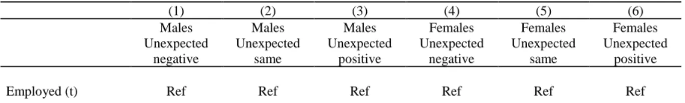
Table 4. Effect of retirement (reported in t) on health shocks (between t and T),

in the full sample

(1) (2) (3) (4) (5) (6)

Males Males Males Females Females Females

Unexpected negative Unexpected same Unexpected positive Unexpected negative Unexpected same Unexpected positive

Employed (t) Ref Ref Ref Ref Ref Ref

Panel A. Shock between t and t+1, constructed as the difference between reported health transition between t and t+1 and expectation reported in t

Completely retired (t) -0.020** -0.000 0.034** -0.025** 0.030** 0.006

(0.010) (0.014) (0.013) (0.010) (0.013) (0.012)

[-23.56%] [14.18%] [-22.50%] [11.25%]

Panel B. Shock between t and t+1, constructed as the difference between computed evolution of SAH between t and t+1 and expectation reported in t

Completely retired (t) -0.023** -0.003 0.023 -0.022* 0.004 0.025**

(0.012) (0.013) (0.014) (0.011) (0.013) (0.012)

[-15.85%] [-13.85%] [9.99%]

Panel C. Shock between t and t+2, constructed as the difference between computed evolution of SAH between t and t+2 and expectation reported in t

Completely retired (t) -0.024 0.008 0.012 -0.027* 0.016 0.014

(0.015) (0.015) (0.016) (0.014) (0.014) (0.014)

[-14.73%]

Panel D. Shock between t and t+1, constructed as the difference between evolution of the PCS between t and t+1 and expectation reported in t

Completely retired (t) -0.005 -0.029** 0.032** -0.022** 0.005 0.009

(0.011) (0.014) (0.014) (0.011) (0.013) (0.013)

[-12.11%] [10.59%] [-15.21%]

Panel E. Shock between t and t+2, constructed as the difference between evolution of the PCS between t and t+2 and expectation reported in t

Completely retired (t) -0.019 0.009 0.026* -0.007 -0.015 0.030**

(0.013) (0.016) (0.016) (0.014) (0.015) (0.015)

[9.12%] [12.88%]

Panel F. Shock between t and t+1, constructed as the difference between evolution of the MCS between t and t+1 and expectation reported in t

Completely retired (t) 0.002 -0.018 0.039*** -0.013 -0.006 0.013

(0.010) (0.015) (0.014) (0.011) (0.014) (0.013)

[13.16%]

Panel G. Shock between t and t+2, constructed as the difference between evolution of the MCS between t and t+2 and expectation reported in t

Completely retired (t) -0.006 -0.007 0.029* -0.012 -0.003 0.021

(0.011) (0.016) (0.016) (0.011) (0.015) (0.014)

[9.90%]

Observations 17,880 17,880 17,880 19,630 19,630 19,630

Number of persons 3,306 3,306 3,306 3,653 3,653 3,653

Notes: The following control variables are included: not completely retired (t), never in the workforce (t), age, age square, marital status, household size, the logarithm of household income, and year dummies. Fixed effects are included. Robust standard errors in parentheses. Effects in percentage in brackets. *** p<0.01, ** p<0.05, * p<0.1.

(27)

25

Table 5. Effect of retirement (reported in t) on health shocks (between t+1 and t+2),

in the full sample

(1) (2) (3) (4) (5) (6)

Panel A. Shock between t+1 and t+2, constructed as the difference between reported health transition between t+1 and t+2 and expectation reported in t+1

Completely retired (t)

-0.012 0.003 0.021 -0.025** 0.020 -0.006

(0.011) (0.015) (0.015) (0.011) (0.014) (0.012)

[-22.57%]

Panel B. Shock between t+1 and t+2, constructed as the difference between computed evolution of SAH between t+1 and t+2 and expectation reported in t+1

-0.013 -0.005 0.009 -0.031** -0.004 0.028**

(0.014) (0.015) (0.016) (0.014) (0.014) (0.014)

[-18.35%] [11.68%]

Panel C. Shock between t+1 and t+2, constructed as the difference between evolution of the PCS between t+1 and t+2 and expectation reported in t+1

-0.031** 0.013 0.019 -0.004 -0.022 0.027*

(0.013) (0.015) (0.017) (0.014) (0.014) (0.014)

[-24.45%] [11.84%]

Panel D. Shock between t+1 and t+2, constructed as the difference between evolution of the MCS between t+1 and t+2 and expectation reported in t+1

Completely retired (t) -0.008 0.000 0.019 -0.022* 0.002 -0.002 (0.011) (0.015) (0.017) (0.011) (0.015) (0.014) [-16.08%] Observations 17,244 17,244 17,244 18,850 18,850 18,850 Number of persons 3,177 3,177 3,177 3,519 3,519 3,519

Notes: The following control variables are included: not completely retired (t), never in the workforce (t), age, age square, marital status, household size, the logarithm of household income, and year dummies. Fixed effects are included. Robust standard errors in parentheses. Effects in percentage in brackets.

(28)

26 APPENDIX

(Online-only supplementary material)

APPENDIX A

Table A1. Consistency of self-reported health transition. Bivariate statistics

Males Females

Reported health transition between t and t+1, reported in t+1

Worse Same Better Worse Same Better

Computed evolution of the physical component summary (PCS) between t

and t+1 -3.566 0.031 1.779 -3.706 0.005 2.276

Computed evolution of the mental component summary (MCS) between t

(29)

27

APPENDIX B

Table B1. Retirement (reported in t), health expectations (reported in t), and health evolutions

(between t and T), in the full sample

(1) (2) (3) (4) (5) (6)

EXPECTATION

Expects worse health

Doesn’t know whether health will get worse

Expects same or better health Expects worse health Doesn’t know whether health will get worse

Expects same or better

health

Panel A. Expectation, reported in t

Completely retired (t) 0.021* -0.007 -0.014 -0.001 0.017 -0.016

(0.012) (0.014) (0.012) (0.010) (0.013) (0.011)

Observations 26,429 26,429 26,429 28,946 28,946 28,946

EVOLUTION

Panel B. Reported health transition between t and t+1, reported in t+1

Completely retired (t) -0.020 -0.005 0.025** -0.032*** 0.015 0.016

(0.013) (0.015) (0.010) (0.011) (0.014) (0.011)

Panel C. Computed evolution of Self-Assessed Health (SAH) between t and t+1

Completely retired (t) -0.014 0.011 0.003 -0.026** 0.004 0.022*

(0.013) (0.017) (0.011) (0.012) (0.016) (0.011)

Panel D. Computed evolution of Self-Assessed Health (SAH) between t and t+2

Completely retired (t) -0.011 -0.002 0.013 -0.035** 0.028 0.007

(0.016) (0.019) (0.014) (0.015) (0.018) (0.014)

Panel E. Computed evolution of the Physical Component Summary (PCS) between t and t+1

Completely retired (t) -0.000 -0.018 0.018 -0.022* 0.001 0.021*

(0.012) (0.017) (0.012) (0.012) (0.016) (0.011)

Panel F. Computed evolution of the Physical Component Summary (PCS) between t and t+2

Completely retired (t) -0.030* 0.019 0.012 -0.013 -0.017 0.030**

(0.016) (0.018) (0.013) (0.015) (0.017) (0.013)

Panel G. Computed evolution of the Mental Component Summary (MCS) between t and t+1

Completely retired (t) -0.004 -0.015 0.019 -0.014 0.006 0.008

(0.011) (0.016) (0.012) (0.012) (0.016) (0.012)

Panel H. Computed evolution of the Mental Component Summary (MCS) between t and t+2

Completely retired (t) -0.010 0.010 -0.001 -0.016 0.010 0.007

(0.013) (0.016) (0.014) (0.013) (0.016) (0.014)

Observations 17,905 17,905 17,905 19,679 19,679 19,679

Notes: The following control variables are included: not completely retired (t), never in the workforce (t), age, age square, marital status, household size, the logarithm of household income, and year dummies. Fixed effects are included. Robust standard errors in parentheses. *** p<0.01, ** p<0.05, * p<0.1.

(30)

28 APPENDIX C

Table C1. Retirement (reported in t), health expectations (reported in t+1), and health

evolutions (between t+1 and t+2), in the full sample

(1) (2) (3) (4) (5) (6)

EXPECTATION

health

Panel A. Expectation, reported in t+1

Completely retired (t) 0.012 -0.006 -0.006 0.005 -0.004 -0.001

(0.013) (0.015) (0.013) (0.011) (0.013) (0.011)

Observations 22,710 22,710 22,710 24,994 24,994 24,994

EVOLUTION

Panel B. Reported health transition between t+1 and t+2, reported in t+2

Completely retired (t) -0.013 0.014 -0.001 -0.026** 0.033** -0.007

(0.013) (0.015) (0.010) (0.013) (0.015) (0.011)

Panel C. Computed evolution of Self-Assessed Health (SAH) between t+1 and t+2

Completely retired (t) -0.011 -0.002 0.013 -0.035** 0.028 0.007

(0.016) (0.019) (0.014) (0.015) (0.018) (0.014)

Panel D. Computed evolution of the Physical Component Summary (PCS) between t+1 and t+2

Completely retired (t) -0.030* 0.019 0.012 -0.013 -0.017 0.030**

(0.016) (0.018) (0.013) (0.015) (0.017) (0.013)

Panel E. Computed evolution of the Mental Component Summary (MCS) between t+1 and t+2

Completely retired (t) -0.010 0.010 -0.001 -0.016 0.010 0.007

(0.013) (0.016) (0.014) (0.013) (0.016) (0.014)

Observations 17,905 17,905 17,905 19,679 19,679 19,679

Notes: The following control variables are included: not completely retired (t), never in the workforce (t), age, age square, marital status, household size, the logarithm of household income, and year dummies. Fixed effects are included. Robust standard errors in parentheses.

(31)

29

APPENDIX D: Restricted sample

Table D1. Retirement (reported in t), health expectations (reported in t), and health evolutions

(between t and T), in the restricted sample

(1) (2) (3) (4) (5) (6)

EXPECTATION

health

Panel A. Expectation, reported in t

Completely retired (t) 0.035** -0.017 -0.018 0.006 0.010 -0.016

(0.014) (0.017) (0.015) (0.013) (0.016) (0.014)

Observations 23,839 23,839 23,839 25,010 25,010 25,010

EVOLUTION

Panel B. Reported health transition between t and t+1, reported in t+1

Completely retired (t) -0.018 -0.010 0.028** -0.034** 0.027 0.007

(0.015) (0.018) (0.012) (0.015) (0.017) (0.013)

Panel C. Computed evolution of Self-Assessed Health (SAH) between t and t+1

Completely retired (t) -0.008 0.001 0.007 -0.029** 0.023 0.005

(0.015) (0.021) (0.014) (0.014) (0.019) (0.013)

Panel D. Computed evolution of Self-Assessed Health (SAH) between t and t+2

Completely retired (t) -0.001 0.000 0.001 -0.049** 0.050** -0.002

(0.021) (0.024) (0.016) (0.019) (0.022) (0.017)

Panel E. Computed evolution of the Physical Component Summary (PCS) between t and t+1

Completely retired (t) -0.019 0.002 0.017 -0.017 -0.001 0.018

(0.015) (0.021) (0.014) (0.015) (0.019) (0.013)

Panel F. Computed evolution of the Physical Component Summary (PCS) between t and t+2

Completely retired (t) -0.039** 0.028 0.012 -0.006 -0.028 0.033**

(0.019) (0.023) (0.016) (0.019) (0.021) (0.016)

Panel G. Computed evolution of the Mental Component Summary (MCS) between t and t+1

Completely retired (t) -0.012 -0.008 0.020 -0.009 0.016 -0.008

(0.013) (0.019) (0.014) (0.014) (0.019) (0.014)

Panel H. Computed evolution of the Mental Component Summary (MCS) between t and t+2

Completely retired (t) -0.029* 0.037* -0.009 0.002 0.005 -0.007

(0.016) (0.020) (0.017) (0.015) (0.020) (0.017)

Observations 15,963 15,963 15,963 16,839 16,839 16,839

Notes: In the restricted sample, we drop individuals who retire several times or come back to work after retirement. The following control variables are included: not completely retired (t), never in the workforce (t), age, age square, marital status, household size, the logarithm of household income, and year dummies. Fixed effects are included. Robust standard errors in parentheses.

(32)

30

Table D2. Effect of retirement (reported in t) on health shocks (between t and T), in the

restricted sample

(1) (2) (3) (4) (5) (6)

Panel A. Shock between t and t+1, constructed as the difference between reported health transition between t and t+1 and expectation reported in t

-0.026** -0.008 0.049*** -0.039*** 0.040** -0.001

(0.011) (0.017) (0.016) (0.012) (0.017) (0.015)

Panel B. Shock between t and t+1, constructed as the difference between Self-Assessed Health (SAH) evolution between t and t+1 and expectation reported in t

-0.018 -0.012 0.049*** -0.023* -0.002 0.039***

(0.014) (0.017) (0.017) (0.014) (0.016) (0.015)

Panel C. Shock between t and t+2, constructed as the difference between Self-Assessed Health (SAH) evolution between t and t+2 and expectation reported in t

-0.024 0.010 0.024 -0.033* 0.009 0.032*

(0.019) (0.018) (0.019) (0.018) (0.018) (0.018)

Panel D. Shock between t and t+1, constructed as the difference between the Physical Component Summary (PCS) evolution between t and t+1 and expectation reported in t

-0.024** -0.027 0.050*** -0.026* 0.009 0.009

(0.012) (0.017) (0.017) (0.014) (0.016) (0.015)

Panel E. Shock between t and t+2, constructed as the difference between the Physical Component Summary (PCS) evolution between t and t+2 and expectation reported in t

-0.031* 0.017 0.039** -0.009 -0.030* 0.037**

(0.016) (0.019) (0.019) (0.018) (0.018) (0.019)

Panel F. Shock between t and t+1, constructed as the difference between the Mental Component Summary (MCS) evolution between t and t+1 and expectation reported in t

-0.009 -0.030* 0.059*** -0.018 -0.008 0.005

(0.012) (0.018) (0.017) (0.013) (0.017) (0.016)

Panel G. Shock between t and t+2, constructed as the difference between the Mental Component Summary (MCS) evolution between t and t+2 and expectation reported in t

Completely retired (t) -0.020 -0.005 0.057*** -0.005 -0.024 0.019 (0.013) (0.020) (0.019) (0.014) (0.019) (0.018) Observations 15,941 15,941 15,941 16,800 16,800 16,800 Number of persons 3,039 3,039 3,039 3,212 3,212 3,212

Notes: In the restricted sample, we drop individuals who retire several times or come back to work after retirement. The following control variables are included: not completely retired (t) and never in the workforce (t), age, age square, marital status, household size, the logarithm of household income, and year dummies. Fixed effects are included. Robust standard errors in parentheses.

(33)

31

APPENDIX E: Shocks between t-1 and t

Table E1. Effect of retirement (reported in t) on health shocks (between t-1 and t), in the full

sample

(1) (2) (3) (4) (5) (6)

Panel A. Shock between t-1 and t, constructed as the difference between reported health transition between t-1 and t and expectation reported in t-1

Completely retired (t) -0.003 -0.021 0.040*** 0.003 0.015 -0.016

(0.009) (0.014) (0.013) (0.009) (0.013) (0.011)

Panel B. Shock between t-1 and t, constructed as the difference between computed evolution of SAH between t-1 and t and expectation reported in t-1

Completely retired (t) 0.002 -0.003 0.027** -0.012 -0.004 0.021*

(0.011) (0.014) (0.014) (0.011) (0.013) (0.011)

Panel C. Shock between t-1 and t, constructed as the difference between evolution of the PCS between t-1 and t and expectation reported in t-1

Completely retired (t) 0.012 -0.025* 0.039*** -0.005 0.007 -0.001

(0.010) (0.014) (0.014) (0.010) (0.013) (0.012)

Panel D. Shock between t-1 and t, constructed as the difference between evolution of the MCS between t-1 and t and expectation reported in t-1

Completely retired (t) 0.002 -0.033** 0.053*** 0.010 -0.017 0.012

(0.010) (0.014) (0.014) (0.010) (0.013) (0.012)

Observations 21,764 21,764 21,764 23,883 23,883 23,883

Notes: Controls for not completely retired (t) and for never in the workforce (t) are included. The following control variables are included: age, age square, marital status, household size, the logarithm of household income, and year dummies. Fixed effects are included. Robust standard errors in parentheses.

(34)

32

APPENDIX F: Additional controls

Table F1. Main model including lagged shocks, in the restricted sample

(1) (2) (3) (4) (5) (6)

Completely retired (t) -0.024* -0.010 0.061*** -0.051*** 0.052*** 0.004

(0.014) (0.022) (0.020) (0.015) (0.019) (0.018)

Lagged shocks and other changes

Unexpected negative Ref Ref Ref Ref Ref Ref

Unexpected same 0.104*** -0.091*** 0.008 0.124*** -0.072*** -0.046***

(0.015) (0.017) (0.015) (0.013) (0.015) (0.013)

Unexpected positive 0.077*** -0.016 -0.064*** 0.096*** 0.008 -0.101***

(0.015) (0.018) (0.017) (0.014) (0.015) (0.015)

Expected negative: Expects worse health & Health is worse

0.053*** -0.018 0.047** 0.099*** -0.042** 0.050**

(0.018) (0.019) (0.023) (0.020) (0.016) (0.021)

Expected same or better health & Health is the same

0.103*** -0.009 -0.024 0.121*** 0.017 -0.042***

(0.015) (0.018) (0.015) (0.014) (0.015) (0.013)

Expected same or better health & Health is better

0.075*** -0.045** -0.003 0.108*** 0.004 -0.034**

(0.020) (0.023) (0.021) (0.018) (0.019) (0.016)

Observations 13,720 13,720 13,720 14,495 14,495 14,495

Notes: In the restricted sample, we drop individuals who retire several times or come back to work after retirement. The explained variable is the shock between t and t+1, constructed as the difference between reported health transition between t and t+1 and expectation reported in t. The explanatory variable is the shock between t-1 and t, constructed as the difference between reported health transition between 1 and t and expectation reported in t-1. The following control variables are included: not completely retired (t), never in the workforce (t), age, age square, marital status, household size, the logarithm of household income, and year dummies. Fixed effects are included. Robust standard errors in parentheses.

(35)

33

Table F2. Main model including lagged self-assessed health, in the restricted sample

(1) (2) (3) (4) (5) (6)

Completely retired (t) -0.019 -0.003 0.041** -0.036*** 0.034* 0.001 (0.012) (0.019) (0.017) (0.014) (0.018) (0.016) Self-assessed health (t-1) Poor -0.030 -0.027 0.117*** -0.123*** -0.019 0.141*** (0.023) (0.024) (0.030) (0.022) (0.022) (0.028) Fair -0.029** 0.001 0.045*** -0.068*** -0.010 0.084*** (0.012) (0.016) (0.017) (0.013) (0.016) (0.015) Good -0.002 -0.009 0.027*** -0.020*** 0.012 0.028*** (0.007) (0.011) (0.010) (0.007) (0.011) (0.009)

Very good Ref Ref Ref Ref Ref Ref

Excellent 0.001 -0.007 -0.050*** 0.016 -0.025* -0.015

(0.007) (0.016) (0.015) (0.011) (0.015) (0.010)

Observations 17,096 17,096 17,096 18,028 18,028 18,028

Notes: In the restricted sample, we drop individuals who retire several times or come back to work after retirement. The following control variables are included: not completely retired (t), never in the workforce (t), age, age square, marital status, household size, the logarithm of household income, and year dummies. Fixed effects are included. Robust standard errors in parentheses.

(36)

34

APPENDIX G: Longitudinal weights

Table G1. Main model using longitudinal weights, in the restricted sample

(1) (2) (3) (4) (5) (6)

Completely retired (t) -0.009 -0.017 0.041** -0.041** 0.061*** -0.007

(0.015) (0.023) (0.020) (0.016) (0.021) (0.018)

Observations 13,920 13,920 13,920 14,938 14,938 14,938

Notes: In the restricted sample, we drop individuals who retire several times or come back to work after retirement. The following control variables are included: not completely retired (t), never in the workforce (t), age, age square, marital status, household size, the logarithm of household income, and year dummies. Fixed effects are included. Longitudinal weights are also included. Robust standard errors in parentheses.

(37)

35

APPENDIX H: Event studies

We also display the results in the form of event studies. We enlarge the window of analysis and look at the dynamics of health shocks before and after retirement, using the following regression:

Yi,(t-1,t) = β-4.R-4,i,t + β-3.R-3,i,t + β-2.R-2,i,t + β-1.R-1,i,t (3) + β0.R0,i,t + β+1.R+1,i,t + β+2.R+2,i,t + β+3.R+3,i,t + β+4.R+4,i,t + β+5.R+5,i,t

+ Xi,t.δ + ρt + αi + εi,t-1,t

The left-hand side variable captures shocks between t-1 and t.

To pick up anticipation, we split the group of people who are not completely retired into five groups: individuals who will transition to retirement in the next 5 years or more, in the next 3-4 years, in the next 2-3 years, in the next 1-2 years, and in the next 0-1 year. We create the

corresponding dummy variables R-5, R-4, R-3, R-2, and R-1. Individuals who will transition to

retirement in the next 5 years or more (R-5) serve as the reference category. To estimate

adaptation, we divide retirees into six groups: those who have been retired for 0-1 years, 1-2 years, and so on up to those who have been retired for 5 years or more. The corresponding dummy variables are R0, R+1, R+2, R+3, R+4, and R+5.

Equation (3) is estimated for a smaller sample than Equation (1) (in the manuscript) due to missing information on the exact year of the retirement transition for some individuals.

Figure H1 displays estimates of anticipation and adaptation to retirement, in terms of shocks, following Equation (3). Each point represents the value of the coefficient associated with a specific lag or lead in the regression of health shock. These coefficients are estimated with reference to the situation where people will retire in more than five years (on the horizontal