HAL Id: hal-02332239
https://hal.archives-ouvertes.fr/hal-02332239
Submitted on 24 Oct 2019
HAL is a multi-disciplinary open access
archive for the deposit and dissemination of
sci-entific research documents, whether they are
pub-lished or not. The documents may come from
teaching and research institutions in France or
abroad, or from public or private research centers.
L’archive ouverte pluridisciplinaire HAL, est
destinée au dépôt et à la diffusion de documents
scientifiques de niveau recherche, publiés ou non,
émanant des établissements d’enseignement et de
recherche français ou étrangers, des laboratoires
publics ou privés.
Is a simplified Finite Element model of the gluteus
region able to capture the mechanical response of the
internal soft tissues under compression?
Aurélien Macron, Hélène Pillet, Jennifer Doridam, Isabelle Rivals,
Mohammad Javad Sadeghinia, Alexandre Verney, Pierre-Yves Rohan
To cite this version:
Aurélien Macron, Hélène Pillet, Jennifer Doridam, Isabelle Rivals, Mohammad Javad Sadeghinia, et
al.. Is a simplified Finite Element model of the gluteus region able to capture the mechanical response
of the internal soft tissues under compression?. Clinical Biomechanics, Elsevier, 2020, 71, pp.92-100.
�10.1016/j.clinbiomech.2019.10.005�. �hal-02332239�
1
Is a simplified Finite Element model of the
1
gluteus region able to capture the mechanical
2
response of the internal soft tissues under
3
compression?
4
Aurélien Macron
1,3, Hélène Pillet
1, Jennifer Doridam
1, Isabelle Rivals
4,5,
5
Mohammad Javad Sadeghinia
1,6, Alexandre Verney
2, Pierre-Yves Rohan
16
1 Institut de Biomécanique Humaine Georges Charpak, Arts et Métiers ParisTech, 151 bd de l'Hôpital, 75013.
7
Paris, France.
8
2 CEA, LIST, Interactive Robotics Laboratory, F-91191 Gif-sur-Yvette, France.
9
3 Univ. Grenoble Alpes, CEA, LETI, CLINATEC, MINATEC Campus, 38000 Grenoble, France.
10
4 Sorbonne Université, INSERM, UMRS1158 Neurophysiologie Respiratoire Expérimentale et Clinique, Paris,
11
France.
12
5 Equipe de Statistique Appliquée, ESPCI Paris, PSL Research University,, Paris, France.
13
6 School of Mechanical Engineering, College of Engineering, University of Tehran, Tehran, Iran.
14
15
16
Keywords: Deep Tissue Injury; Pressure Ulcer; Subject specific; Buttock, Sitting, Finite Element Analysis
17
18
Word count: (Abstract: 210 words; Main text: 3856 words)
19
Original Article Submission (less than 4000 words), Word count (introduction through conclusion): 3827
20
2
Abstract
22
Background: Internal soft tissue strains have been shown to be one of the main factors responsible for the
23
onset of Pressure Ulcers and to be representative of its risk of development. However, the estimation of this
24
parameter using Finite Element (FE) analysis in clinical setups is currently hindered by costly acquisition,
25
reconstruction and computation times. Ultrasound (US) imaging is a promising candidate for the clinical
26
assessment of both morphological and material parameters.
27
Method: The aim of this study was to investigate the ability of a local FE model of the region beneath the
28
ischium with a limited number of parameters to capture the internal response of the gluteus region predicted
29
by a complete 3D FE model. 26 local FE models were developed, and their predictions were compared to those
30
of the patient-specific reference FE models in sitting position.
31
Findings: A high correlation was observed (R= 0.90, p-value < 0.01). A sensitivity analysis showed that the
32
most influent parameters were the mechanical behaviour of the muscle tissues, the ischium morphology and
33
the external mechanical loading.
34
Interpretation: Given the progress of US for capturing both morphological and material parameters, these
35
results are promising because they open up the possibility to use personalised simplified FE models for risk
36
estimation in daily clinical routine.
37
38
3
Introduction
40
Pressure Ulcers (PU) are painful, slow-healing wounds that develop during periods of prolonged
41
immobility, and that are likely to deteriorate the quality of life of people with poor mobility and sensitivity.
42
They can develop either superficially and progress inward or initiate at the deep tissues and progress outward
43
(called Deep Tissue Injury) depending on the nature of the surface loading (Bouten et al., 2003). The first type
44
is predominantly caused by shear stresses and is fairly easily detected and treated before it becomes
45
dangerous. The latter type, caused by sustained compression of the tissue, originates subcutaneously,
46
generally close to bony prominences (NPUAP/EPUAP, 2009). Although DTI represents a small proportion of
47
PUs (<10%) this latter type is considered especially harmful because layers of muscle, fascia, and
48
subcutaneous tissue may suffer substantial necrosis equivalent to a category III or IV PU with variable
49
prognosis.
50
Since the pioneer work of (Daniel et al., 1981; Kosiak, 1961; Reswick and Rogers, 1976) establishing
51
the dependence of PU development on both external pressure and time, interface pressure mapping has been
52
widely used in PU prevention. Although clinically useful, interface pressure monitoring is not predictive
53
enough of the risk of PU development. Indeed, it is now indisputable that there are at least two damage
54
mechanisms, which play an important role in PU development (Oomens et al., 2015): (i) mechanically induced
55
capillary occlusions that lead to low oxygen concentration in the tissue triggering a cascade of inflammatory
56
signals that culminate in ulceration (Gawlitta et al., 2007; Kosiak, 1959; Loerakker et al., 2011; Sree et al.,
57
2019a). This process can occur even for very small values of soft tissue strain and takes several hours before
58
the first signs of cell damage can be detected (Breuls et al., 2003; Loerakker et al., 2010; Stekelenburg et al.,
59
2007, 2006). (ii) “direct deformation damage” involving cells damage by direct (shear) deformation (Breuls et
60
al., 2003; Ceelen et al., 2008; Stekelenburg et al., 2006). This damage can be evident when the threshold for
61
deformation damage exceeds the normal physiological values experienced in daily life and can be detected in
62
a period of minutes (Ceelen et al., 2008; Loerakker et al., 2010). In addition, microclimate (skin surface
63
temperature and skin moisture) is also suspected to play a key role in PU causation (Gefen, 2011; Zeevi et al.,
64
2017) but the extent of the contribution and its interaction with sustained tissue deformations have yet to be
65
quantified.
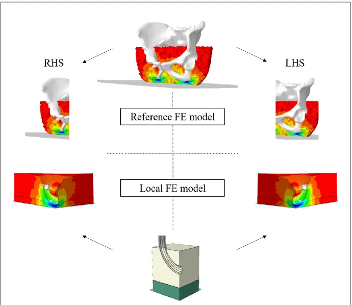
4
Estimating the internal mechanical conditions within loaded soft tissues has the potential of
67
improving the management and prevention of PU and several Finite Element (FE) models have been
68
developed for more than 20 years to bridge the gap between external pressures and internal strains (Al-Dirini
69
et al., 2016; Linder-Ganz et al., 2009; Luboz et al., 2017; Moerman et al., 2017). Along these lines, we recently
70
proposed a new methodology to build a 3D patient-specific FE model based on the combination of ultrasound
71
(US), bi-planar x-ray radiographies and optical scanner (Macron et al., 2018) to estimate internal strains in
72
sitting position. However, the clinical use of such models is currently hindered by costly acquisition,
73
reconstruction and computation times. In contrast, there is a consensus in the results reported in the
74
literature that the clinically relevant mechanical response is localised under the ischium. This strongly
75
suggests that a local model of the soft tissue under the ischium could account for the major part of the
76
mechanisms. Recent evidence also suggest that response to damage, as observed by MRI, starts at some
77
distance from the deformation (Nelissen et al., 2018), highlighting the importance of evaluating the
78
mechanical response in 3 dimensions.
79
Only a few contributions have tried to explore this avenue in the literature. In 2011, Portnoy et al.
80
developed a simple 2D analytical model (Portnoy et al., 2011) based on the Hertz contact model. Promising
81
results have been reported regarding the comparison between the maximal Von Mises stress estimated by
82
their local model and that predicted by a full 3D FE model developed by Linder-Ganz (Linder-Ganz et al.,
83
2008a). In a sample of 11 heathy subjects, a Pearson correlation of 0.4 was obtained. However, the
84
consistency of the results can be expected to be improved by adding complementary parameters that have
85
been identified as predominant in the internal mechanical response of the ischial region, such as the radius of
86
the ischium (Agam and Gefen, 2007) and the mechanical behaviour of the soft tissue (Luboz et al., 2014).
87
Moreover, shear strains estimations also seem essential and were not reported in their work. Thus, there is a
88
need to extend this analytical approach to a more comprehensive model of the behaviour of the soft tissue in
89
the ischial region with the additional constraint that it should be based on parameters that can be routinely
90
obtained in a clinical environment.
91
At the same time, recent studies showed the potential of US imaging for the characterization of
92
morphological parameters. In a recent paper, Akins et al. reported that the measurement of the adipose and
93
muscle tissue thicknesses in the vicinity of the ischium using US was both reliable (ICC = 0.948) and highly
5
correlated with MRI assessment (r = 0.988 and 0.894 for the muscle and the adipose tissues
95
respectively)(Akins et al., 2016). On the contrary, the measurement of the radius of curvature of the ischium
96
was reported to have a poor inter operator reliability be it using US (ICC = -0.028) (Akins et al., 2016) or MRI
97
(ICC = 0.214) (Swaine et al., 2017). However, there is a high interest in the community for developing both the
98
US system (Bercoff et al., 2004; Gennisson et al., 2013, 2010) and clinical protocols that are suited to reliable
99
parameter assessment (Swaine et al., 2017). Similar efforts are also being made to characterize material
100
parameters (Makhsous et al., 2008). This makes US a promising candidate to substitute MR imaging for
101
clinically feasible assessment of both morphological and material parameters needed for the prevention of PU.
102
In this perspective, we propose here to evaluate the ability of a local model of the region beneath the
103
ischium to capture the maximum shear strain inside the muscle tissue. This evaluation will be made by
104
comparing the response provided by this model to the one predicted by a previously developed complete 3D
105
FE model of the buttock (Macron et al., 2018). In addition, the relative impact of the different parameters on
106
the local model response will be analysed.
107
108
6
Methods
109
For the sake of clarity, the experimental material and the construction of the reference FE model (Macron
110
et al., 2018) are briefly recalled hereunder in section 1.
111
-1- Reference FE model
112
13 subject-specific FE models (8 men and 5 women; age: 26 ± 5 yrs, weight: 70 ± 9 kg, BMI: 22.6 ± 3.4
113
kg/m²) models (reference) were generated from previous experiments detailed in (Macron et al., 2018).
114
3D reconstruction of the pelvis was performed from biplanar X-rays in an unloaded sitting position. The
115
external envelope was reconstructed from the optical scan acquisition, and the adipose tissue thickness was
116
directly measured on the US image in the unloaded configuration.
117
The skin, fat and muscle tissues were each modelled with a first order Ogden hyperelastic material model
118
(Simo and Taylor, 1991). Material parameters for the skin were based on values reported in the literature
119
(Luboz et al., 2014). For the fat and the muscle, 𝛼 was arbitrarily fixed to 5 (Oomens et al., 2016) and the shear
120
modulus 𝜇 was calibrated using Finite Element Updating to fit the experimental ischial tuberosity sagging
121
(Macron et al., 2018). The shear moduli of the adipose and muscle tissue will subsequently be referred to as
122
𝝁𝑭 and 𝝁𝑴.
123
For the boundary conditions, all the degrees of freedom (DOF) of the pelvis were fixed except the vertical
124
displacement. The experimental vertical force measured in the loaded sitting position was applied at the
125
centre of mass of the pelvis.
126
The nodes at the different interfaces (bone/muscle, muscle/fat, and fat/skin) of the model were tied. A
127
friction contact between the rigid plane and the skin surface was defined using a penalty algorithm. The
128
friction coefficient was set to 0.4 (Al-Dirini et al., 2016).
129
-2- Local FE model
130
a. Extraction of model parameters
131
The parameters necessary for the construction of the local FE model were quantified for the 13
132
subjects.
7
Two radii of curvature were calculated from the 3D pelvis reconstruction. For each side of the pelvis,
134
the extreme node of the surface mesh with the lowest vertical coordinate was identified. A region of interest
135
containing all the nodes at less than 8 mm of the extreme node was then defined. Several planes containing
136
the vertical direction were generated. The orientation of their normal vectors was distributed between 0 and
137
170 degrees by 10 degree increments. Each plane intersected the region of interest and allowed to define a set
138
of nodes which were used to extract a radius from a circular regression. The minimal radius obtained across
139
the planes is called R1. The radius of curvature R2 in the orthogonal plane was then extracted.
140
The fat thickness eF was extracted from the US image in the unloaded sitting position. The total
141
subdermal soft tissue thickness under the ischium was extracted from the sagittal x-ray image in the unloaded
142
sitting position, and the muscle thickness eM was calculated as the difference between the total thickness and
143
the fat thickness.
144
The static contact pressure distribution at the skin/seat interface computed by the reference FE
145
model in the loaded sitting position was used to extract the net reaction force. The pressure distribution was
146
first interpolated over a regular grid with 1 mm spatial resolution. The contact pressure of the nearest FE
147
surface node of the reference model was assigned to each point of the grid. The nodal vector force associated
148
to each grid node was then computed by multiplying the nodal pressure with the surface area (1 mm²). A net
149
reaction force F was calculated as the vector sum of the nodal forces on the left-hand side (LHS) and
right-150
hand side (RHS).
151
To summarize, seven parameters were considered: 𝝁𝑭, 𝝁𝑴, R1, R2, eF, eM, F.
152
b. Finite Element modelling
153
26 local FE models were developed to represent the mechanical response of the LHS and RHS of the
154
13 patient-specific reference FE models (Figure 1).
8
156
Figure 1: Reference FE model (top) and associated LHS and RHS local FE models (bottom) for one subject.
157
The local FE model geometry is presented in Figure 2. The ischial tuberosity is represented by a torus
158
generated by the revolution of a parametric curve C containing a portion of a circle of radius R2 swept by a
159
semi-disc of radius R1. A box of height h, length L and width L was defined to represent the whole subdermal
160
soft tissue (fat + muscle). A convergence study showed that, above an L/h ratio of 2, the solution was not
161
affected. A boolean operation was performed to subtract the ischium from the soft tissue volume. A skin layer
162
of 1 mm thickness was defined. A rigid horizontal plane was created to model the seat support.
9
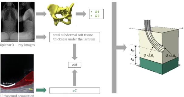
164
Figure 2: Local FE model geometry generated from the 4 geometric parameters R1, R2, eF, eM extracted from the ultrasound
165
and bi-planar x-ray images. The ischial tuberosity is represented by a torus generated by the revolution of a circle of radius R1
166
(minor radius of the torus) around a portion of a circle of radius R2 (major radius of the torus). eM and eF are used to define
167
the muscle and fat thicknesses respectively.
168
The soft tissues were meshed using linear tetrahedral elements with hybrid formulation (C3D4H) in
169
ABAQUS Finite Element Analysis software (ABAQUS Inc., Providence, RI, USA). The pelvis was assumed to be
170
rigid and meshed with triangular shell elements. The same constitutive laws and material parameters as those
171
defined in section 1 for the reference FE model were used for each subject. Likewise, for the boundary
172
conditions, all the DOF of the ischium were fixed except the vertical displacement. The force F was applied to
173
the ischium. Only a quarter of the model was considered and the remainder was completed using the
174
symmetry constraints (Figure 2).
175
c. Quantity of interest
176
The strains were post-processed from the principal stretches 𝜆𝑖 (𝑖 = 1,2,3). Based on these, the
177
principal Green-Lagrange strains were calculated as: 𝐸𝑖= (𝜆𝑖2−1)
2 and the principal shear strains were then
178
computed as:179
𝐸𝑠ℎ𝑒𝑎𝑟= 1 2∗ max (|𝐸1− 𝐸2|, |𝐸2− 𝐸3|, |𝐸3− 𝐸1|)180
The third principal strain component 𝐸3 corresponds to the principal compressive strain. This quantity
181
will be referred to hereafter as 𝐸𝑐𝑜𝑚𝑝.
182
10
In line with (Bucki et al., 2016; Luboz et al., 2017), a “cluster analysis” was performed to investigate
183
volumes of the model that are in given intervals of maximum shear strain. Clusters were defined as the union
184
of adjacent elements verifying the following criteria: (i) 𝐸𝑠ℎ𝑒𝑎𝑟 above 75% and (ii) 𝐸𝑐𝑜𝑚𝑝 above 45%. These
185
correspond to the damage thresholds reported by (Ceelen et al., 2008) for the muscle tissue. However, unlike
186
(Bucki et al., 2016) who investigated the response in both muscle and fat, only the muscle tissue was
187
investigated here.
188
To be able to compare our results with those of the literature, the Engineering strain was defined as
189
follows: 𝜀𝑖= 𝜆𝑖− 1. The reason for using Cauchy’s strain definition instead of the standard Green-Lagrange
190
strain definition is that the latter poorly describes large compression (with a maximum compressive strain
191
limit of 50%). As previously, the principal shear strains were computed from the principal Engineering
192
strains:193
𝜀𝑠ℎ𝑒𝑎𝑟 = 1 2∗ max (|𝜀1− 𝜀2|, |𝜀2− 𝜀3|, |𝜀3− 𝜀1|)194
For the reference FE model, the maximum principal shear strain 𝜀𝑚𝑎𝑥 = max (𝜀𝑠ℎ𝑒𝑎𝑟) in the cluster
195
with the largest volume inside the muscle tissue was extracted and analysed. For the local FE model, the
196
maximum principal shear strain 𝜀𝑚𝑎𝑥= max(𝜀𝑠ℎ𝑒𝑎𝑟) was computed from the elements inside the muscle
197
tissue and on the axis of symmetry.
198
-3- Correlation between the reference and the local model
199
The correlation between the maximum principal shear strain predictions of the reference and local FE
200
models was quantified with Pearson’s correlation coefficient on the 13 patients (left and right).
201
-4- Sensitivity Analysis of the local model
202
In order to investigate the impact of the input parameters (R1, R2, eM, eF, 𝝁𝑴, 𝝁𝑭 and F) on the
203
maximum shear strain predicted by the local model,we chose to emulate the latter with a polynomial model.
204
using the same parameters. The ranges over which the 𝑚 = 7 parameters were to be varied were defined
205
between their minimum and maximum value observed in the 13 subjects (LHS and RHS), see Table 1. After
206
normalization in [-1; 1], experimental points were chosen according to a three-level full factorial design
207
resulting in 37 combinations (i.e. 2187 FE model simulations).
208
11
Table 1: Levels of the parameters used for the sensitivity analysis.209
Parameter
Level of the parameter
Min Level (-1) Mid-Level Max Level (+1)
R1 5 (mm) 7 (mm) 9 (mm)
R2 15 (mm) 39 (mm) 63 (mm)
eM 19 (mm) 29 (mm) 39 (mm)
eG 9 (mm) 22 (mm) 35 (mm)
uM 1.0 (kPa) 4.5 (kPa) 8.0 (kPa)
uG 2.8 (kPa) 5.4 (kPa) 8.0 (kPa)
F 48 (N) 77.5 (N) 107 (N)
210
The output of the local FE model being noiseless, there is in principle no lower bound to the mean
211
squared residuals of candidate models other than zero. In the following, the use of a polynomial model of
212
degree at most equal to two will used:
213
214
The maximum value of two for the degree will be justified in section 2 of the results using the errors of the
215
local FE model with respect to the reference FE model obtained on the 13 subjects (left and right).
216
The sensitivity of the model to each input (linear term, square, order-two interaction) can be simply
217
defined as the percentage of variance due to this input. Assuming the parameters (R1, R2, eM, eF, 𝝁𝑴, 𝝁𝑭 and
218
F) independent and uniformly distributed in [-1, 1] (i.e. with second and fourth order moments of respectively
219
1/3 and 4/45), we have:
220
221
For the degree 1 model, the sensitivity to the i-th parameter is hence given by the following percentage:
222
si= var(qixi)= qi2 var(xi)= qi2´1 3 sii= var(qiixi2 )= qii2 var(xi2 )= qii2´ 4 45 sij= var(qijxixj)= qij2 var(xi) var(xj)= qij2´ 1 9 var(y)= si i=1 må
+ sii i=1 må
+ sij j>iå
i=1 må
ì í ï ï ï ïï î ï ï ï ï ï12
223
For the degree 2 model, the sensitivities to the i-th parameter and to its interaction with parameter j are given
224
by the percentages:225
226
227
Si= si var(y)= qi2 qi2å
Si= si+ sii var(y),Sji= sij var(y)13
Results
228
-1- Subjects and parameters
229
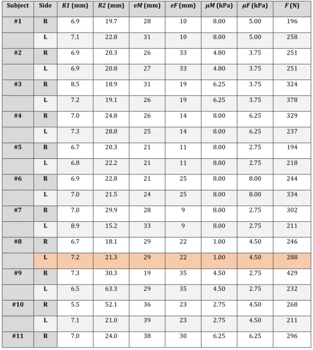
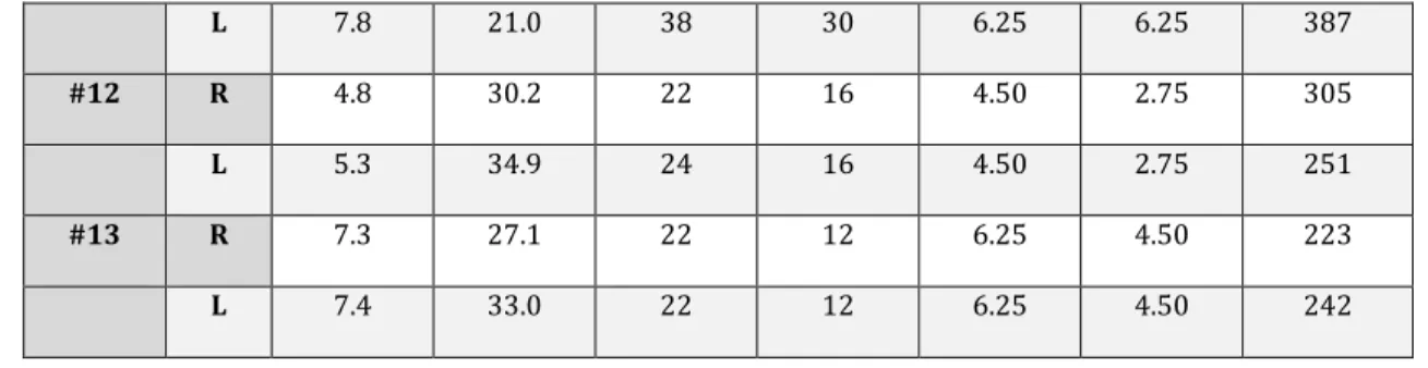
The values of the parameters for the 13 modelled subjects are reported in Table 2 below for each side.
230
The simulation of the local FE model corresponding to the LHS of subject #8 did not converge.
231
Table 2: Characteristics of subjects for each side (right and left). The LHS of subject #8 is indicated in a different color because
232
the simulation of the local FE model did not converge.
233
Subject Side R1 (mm) R2 (mm) eM (mm) eF (mm) µM (kPa) µF (kPa) F (N)
#1 R 6.9 19.7 28 10 8.00 5.00 196 L 7.1 22.8 31 10 8.00 5.00 258 #2 R 6.9 20.3 26 33 4.80 3.75 251 L 6.9 20.8 27 33 4.80 3.75 251 #3 R 8.5 18.9 31 19 6.25 3.75 324 L 7.2 19.1 26 19 6.25 3.75 378 #4 R 7.0 24.8 26 14 8.00 6.25 329 L 7.3 28.8 25 14 8.00 6.25 237 #5 R 6.7 20.3 21 11 8.00 2.75 194 L 6.8 22.2 21 11 8.00 2.75 218 #6 R 6.9 22.8 21 25 8.00 8.00 244 L 7.0 21.5 24 25 8.00 8.00 334 #7 R 7.0 29.9 28 9 8.00 2.75 302 L 8.9 15.2 33 9 8.00 2.75 211 #8 R 6.7 18.1 29 22 1.00 4.50 246 L 7.2 21.3 29 22 1.00 4.50 288 #9 R 7.3 30.3 19 35 4.50 2.75 429 L 6.5 63.3 29 35 4.50 2.75 232 #10 R 5.5 52.1 36 23 2.75 4.50 268 L 7.1 21.0 39 23 2.75 4.50 211 #11 R 7.0 24.0 38 30 6.25 6.25 296
14
L 7.8 21.0 38 30 6.25 6.25 387 #12 R 4.8 30.2 22 16 4.50 2.75 305 L 5.3 34.9 24 16 4.50 2.75 251 #13 R 7.3 27.1 22 12 6.25 4.50 223 L 7.4 33.0 22 12 6.25 4.50 242234
-2- Maximum shear strains and external pressures
235
The bar plot below (Figure 3) summarizes the maximum principal shear strains estimated by the
236
reference FE model and the local FE model for each subject and for each side (right and left). In addition, the
237
external pressure is also plotted with a secondary axis.
238
239
Figure 3: Bar plots representing the maximum shear strains estimated by the local FE model (green) and the reference FE
240
model (red), and the external pressure (blue).
241
As shown on figure 3, the external pressure is poorly correlated to the maximum principal shear
242
strain estimated by the two FE models. For example, subject #10 endures a low pressure on both sides, but
243
suffers high internal strains. On the contrary, subject #1’s left side shows a high pressure associated to a small
244
internal strain.
15
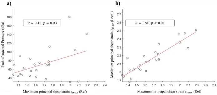
Pearson’s correlation coefficient between 𝜀𝑚𝑎𝑥 estimated by the reference and local FE models was
246
0.90 (𝑝 < 0.01). In contrast, Pearson’s correlation coefficient between 𝜀𝑚𝑎𝑥 estimated by the reference model
247
and the external pressure was 0.43 (𝑝 = 0.03).
248
249
Figure 4: (a) maximum principal shear strains estimated by the reference FE model versus external pressure for the thirteen
250
subjects, (b) maximum principal shear strains estimated by the reference FE model versus the predictions of the local FE
251
model.
252
The results depicted in figure 4(b) show a high linear correlation between the local FE model and the
253
reference FE model, but a poor agreement: the mean squared error between reference and local model
254
predictions equals 0.25. Note that for the sensitivity analysis using a polynomial model emulating the local FE
255
models, since their outputs are noiseless, we need a lower limit for the mean square error between local model
256
and polynomial outputs for the choice of the adequate polynomial complexity. Since even a constant model has
257
smaller mean squared residuals (0.075) than the local FE models, their mean square error of 0.25 cannot be used
258
to select the degree of the polynomial model emulating the local model.
259
However, considering the good linear correlation between the local and the reference model, we can
260
compute the mean squared error obtained after regressing the reference model on the local one, which
261
represents the error achieved by the local model if it were in agreement with the reference model. Thus, it
262
provides a lower limit for the mean squared residuals of candidate polynomial models for the emulation of the
263
local FE model. Numerically, this corrected mean squared error equals 5.7 10-3 .
264
-3- Sensitivity analysis
16
Out of the 2187 simulations, 239 did not converge (11%). A possible reason may be the chosen values for
266
the minimum and maximum parameter values, the minimum muscle shear modulus value in particular.
267
Indeed, a single experimental measure was used to calibrate the material properties of both muscle and
268
adipose tissues by an inverse method. Using the remaining simulations, the coefficients of the degree 1 and
269
degree 2 models were estimated with ordinary least squares. The first order sensitivities to the 7 parameters
270
obtained with the linear model are given in Table 3, in decreasing order of sensitivity.
271
272
273
Table 3 First order sensitivities to the 7 parameters in decreasing order of magnitude.
274
parameters coefficient i 𝑺𝒊(%) 𝜇𝑀 -0.1770 38 𝑅𝐶𝐶𝐼2 -0.1604 31 𝐹 +0.1226 18 𝑅𝐶𝐶𝐼1 -0.1092 10 𝑒𝑀 +0.0213 0.55 𝑒𝐹 +0.0184 0.41 µG -0.0178 0.39275
The mean squared residuals of the linear model (2.0*10-2) largely exceeded the corrected mean squared error
276
of 5.7*10-3 obtained with the comparison to the reference model, so that first order sensitivities might not
277
capture the complexity of the local FE model. Thus, we computed the sensitivities obtained with the
second-278
degree model, see Table 4. Since its mean squared residuals (3.9*10-3) are close to the corrected mean
279
squared error, this model is neither too simple, nor excessively complex. Note that, due to the missing data
280
corresponding to the simulations that did not converge, the experiment matrix is not strictly orthogonal,
281
hence the slight modification of the linear coefficients i when adding the interactions and the squared terms.
282
17
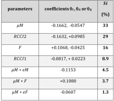
Table 4 Second-order sensitivities (> 1%) in decreasing order of magnitude.283
parameters coefficients I , ii or ij 𝑺𝒊 (%) 𝜇𝑀 -0.1662, -0.0547 33 𝑅𝐶𝐶𝐼2 -0.1632, +0.0985 29 𝐹 +0.1068, -0.0425 16 𝑅𝐶𝐶𝐼1 -0.0817, + 0.0223 8.9 𝜇𝑀 ∗ 𝑒𝑀 -0.1153 4.5 𝜇𝑀 ∗ 𝐹 +0.1080 3.7 𝜇𝑀 ∗ 𝑒𝐹 -0.0607 1.3284
285
18
Discussion
286
The aim of this study was to investigate the ability of a local model of the region beneath the ischium
287
to capture the internal response of the buttock soft tissues predicted by a complete 3D FE model from a
288
limited number of parameters. Our long term ambition is to take advantage of the potential of basic US for the
289
measurement of both morphological and material parameters in daily clinical routine. To this end, we also
290
investigated the relative impact of the main parameters reported in the literature to drive the internal
291
response of the soft tissues.
292
The analysis of the results obtained in this contribution shows the biomechanical response of the
293
internal soft tissues predicted by a local FE model in 13 subjects is similar to the one predicted by the
294
complete and complex reference 3D FE model (Pearson coefficient of 0.90 and p-value < 0.01). Previous
295
attempts to develop and evaluate simplified models built from a limited number of parameters have been
296
reported in the literature (Agam and Gefen, 2007; Oomens et al., 2003; Portnoy et al., 2011). Some of these
297
models focused on analytical solutions of the Hertz contact problem to predict both the peak interface contact
298
pressure at the bone/muscle interface (Agam and Gefen, 2007) and the internal von Mises soft tissue stresses
299
(Portnoy et al., 2011), and displayed a relatively good agreement with patient-specific FE von Mises stresses
300
published by Linder-Ganz et al. on the same 11 patients (R = 0.4) with a relatively low computation time
301
facilitating real-time operation and portability. However, they rely on important assumptions: elasticity of the
302
two contacting bodies, relatively small area of contact in comparison to the size of the geometry modelled.
303
These assumptions particularly hinder models ability to estimate shear strain in the soft tissue, identified as
304
the primary cause of soft tissue breakdown in both animal models and tissue engineered constructs at the cell
305
level. The high correlation obtained in our contribution between the local FE model and the reference FE
306
model for the estimation of the principal shear strain is very promising because, for the first time , it allows to
307
consider the use of such personalised simplified models in daily clinical setup. Moreover, the results obtained
308
in this study confirmed previous observations reported in the literature that external contact pressures are
309
poorly correlated (R=0.43, p=0.3) to the internal local strains endured by soft tissues (Bouten et al., 2003;
310
Chow and Odell, 1978; Dabnichki et al., 1994; Luboz et al., 2014).
19
The sensitivity analysis establishes that the most influential parameter is the mechanical behaviour of
312
the muscle soft tissue, which is in agreement with the conclusion of (Luboz et al., 2014). In particular, the
313
authors observed that a variation of Young’s modulus of the muscle between 40kPa and 160 kPa resulted in a
314
variation of the maximum Von Mises strain of 38.5%. In our study, the shear modulus of the muscle explained
315
33 % of the internal soft tissue response variance. We also observed that changing the mechanical properties
316
of the underlying adipose tissue did not influence the mechanical response of the muscle tissue. This had
317
already been reported by (Oomens et al., 2003). From a clinical perspective, this result supports recent
318
findings that SCI patients with fat infiltration, scarring or spasms puts them at a higher risk for DTI because of
319
increased internal loads in the gluteus muscles in the vicinity of the ischial tuberosities during sitting (Sopher
320
et al., 2011). The maximum shear strain in the muscle tissue is also very sensitive (29%) to the radius of
321
curvature (R2) in the plane perpendicular to the shortest radius of curvature (R1) referred to as radius of
322
curvature in the long axis by (Swaine et al., 2017). This result could be expected because in indentation-like
323
configurations, the geometry of the indentor is known to have a paramount importance. This observation
324
could explain the increasing enthusiasm of the community for the measurement of this anatomical
feature-325
related risk factor using medical imaging (Akins et al., 2016; Linder-Ganz et al., 2008a; Swaine et al., 2017). In
326
the literature however, only (Swaine et al., 2017) represented the ischium using two radii of curvature. Our
327
results confirm that this is essential to consider the variability along both axes in order to properly capture
328
the mechanical response of the soft tissue. The external force explains 16% of the variability of the response.
329
Unlike the other parameters, its measurement is relatively easy even in clinical routine. A particular attention
330
should be paid to the extraction of the force that is transferred to the ischium from the global measurement
331
base on pressure mattresses. Adding the smallest radius of curvature to the above list of parameters allows to
332
explain 82% of the total variability of the mechanical response.
333
The remaining 18% are mainly explained by the interaction between muscle mechanical behavior
334
and (1) muscle thickness (4.5%), (2) external force (3.7%), and (3) fat thickness (1.3%). Thus, considering a
335
fixed muscle mechanical behavior, an increase of the maximum shear strain will result from an increase in the
336
external force and/or a decrease in the muscle and fat thicknesses. This is consistent with the results reported
337
by (Oomens et al., 2003; Portnoy et al., 2011).
20
Limitations and perspectives of this work are detailed herein. First, the fact that local shear strains
339
predicted by the local FE model are all higher than those predicted by the reference FE model strains points at
340
a systematic error. This may be partly due to the fact that approximating the ischial tuberosity by a torus is
341
too gross and leads to biases in the mechanical response. Examination of the ischial tuberosities on the US
342
images revealed that some subjects roughly had a triangular bore rather than a circular bore in shape. As
343
discussed above, in indentation-like configurations, the geometry of the indentor is known to have a
344
paramount importance. As far as the authors are aware of, analysis of the inter-individual variations of the
345
morphological cross section of the ischial tuberosity has never been investigated before and further work is
346
required to improve the geometric approximation of the ischial tuberosity from US images. The systematic
347
error also suggests that, in addition to the choice of the geometric approximation of the ischial tuberosity,
348
other factors involved in the definition and measurement of the principal shear strain in the local FE model
349
might be lacking, their identification requiring further work. Second, the extraction of the material properties
350
using an inverse identification method (for which the optimal parameters are obtained by minimizing the
351
distance between experimental measures and numerical results), although popular for lower limb soft tissues
352
(Affagard et al., 2015; Frauziols et al., 2016; Macron et al., 2018; Rohan et al., 2014; Sadler et al., 2018), is not
353
compatible with clinical implementation because of lengthy solver times for the models and the need for a
354
trained user to develop and interpret the FE model. Ultrasound Elastography, and, in particular, Supersonic
355
Shear Imaging (SSI) technique, is emerging as an innovative tool that could provide a quantitative evaluation
356
of biomechanical properties of soft tissues (Eby et al., 2013; Gennisson et al., 2010; Haen et al., 2017; Vergari
357
et al., 2014). However, to our knowledge and to date, no correlation has been done between shear moduli
358
obtained by Shear Wave Elastography and mechanical properties from classic ex vivo mechanical testing
359
methods. The development of surrogate models that allow equivalent predictions to single FEA solutions,
360
across a broad population with sufficiently reduced computational expense for clinical use (Steer et al., 2019)
361
is a promising alternative that will be explored in future work. Third, the strain damage thresholds (above
362
75% and above 45%) reported in the literature for tissue injury (motivated by the work of (Ceelen et al.,
363
2008; Loerakker et al., 2011) come from animal models and should be considered with some caution since
364
they might not be relevant for humans. Very recently, in an attempt to elucidate the soft tissue injuries leading
365
from pressure-driven ischemia, a computational model linking microvascular collapse to tissue hypoxia in a
21
multiscale model of pressure ulcer initiation has been proposed (Sree et al., 2019a, 2019b) in the context of
367
pressure ulcer formation. These types of models, coupled with recent improvements in ultrasound imaging
368
technologies that allow to measure tissue perfusion in clinical routine, constitute opportunities for elucidating
369
some of the scientific challenges associated with the customization of the injury thresholds.
370
In the present contribution, the authors have used a multimodal approach based on B-mode
371
ultrasound images and low-dose biplanar X-ray images in a non-weight-bearing sitting posture for the fast
372
generation of patient-specific FE models of the buttock. Compared to previously conducted, MRI-based
373
computational models (Al-Dirini et al., 2016; Levy et al., 2017; Levy and Gefen, 2017; Linder-Ganz et al.,
374
2007a, 2008b, 2009; Moerman et al., 2017; Sopher et al., 2010; Zeevi et al., 2017), our protocol suffers from a
375
number of limitations including the poor visibility of B-mode ultrasound for viewing the organization and
376
composition of the buttock soft tissues (muscle groups, tendon, fat pads and ligament borders) and the limited
377
field of view of B-mode ultrasound. However, most MRI-based computational models in the literature model
378
these as a single homogenous material to allow for convergence of tissue geometry and, therefore, clearly fail
379
to take advantage of the capacity of MRI to differentiate between the individual soft tissue structures.
380
Moreover, long acquisition times of MR imaging prevent the representation of a realistic unloaded sitting
381
position without resorting to devices such as: rubber tires (Linder-Ganz et al. 2007), inclined plane (Al-Dirini
382
et al. 2016) and thigh and arms supports (Call et al., 2017). On the contrary, the proposed protocol allows to
383
reproduce the unloaded sitting position easily. Finally, acknowledging the fact that mechanical strains are
384
responsible for deformation-induced damage involved in the initiation of Deep Tissue Injury (DTI), a better
385
assessment of the internal behavior could enable to enhance the modeling of the transmission of loads into
386
the different structures composing the buttock. If MRI is a potential tool for the quantitative evaluation of
387
subdermal soft tissue strains, it has important drawbacks including long acquisition time, examination cost
388
and confined environment. A contrario, in a recent publication (Doridam et al., 2018), we showed the
389
feasibility of using B-mode ultrasound imaging for the quantification of internal soft-tissue strains of buttock
390
tissues in two perpendicular planes during sitting. Further research is currently under progress to develop
391
and validate computational modeling based on ultrasound data alone. This would make additional DTI
392
research more accessible and attainable, and would allow for translational development of future
patient-393
specific risk assessment tools.
22
This work proposed a promising new step towards estimating internal mechanical conditions within
395
loaded soft tissues from data potentially compatible with daily clinical routine. While additional experimental
396
validation is required for the design of appropriate protocols for the robust extraction of both the
397
morphological parameters of interest and the characterization of the mechanical behavior of the soft tissue of
398
interest, this work opens a way to overcome the barriers to clinical implementation of biomechanical metrics
399
as surrogates for improving the management and prevention of PU including difficulty in obtaining imaging
400
data.
401
402
Author contributions statement
403
AM, HP and PYR contributed to the conception and design of the study; JD, MJS and AM performed experiment
404
and data collection; IR performed the statistics. All the authors contributed to data interpretation and
405
preparation of the manuscript. All authors approved the final version of the manuscript.
406
407
Conflict of interest statement
408
The authors certify that no conflict of interest is raised by this work.
409
Acknowledgments
410
This work was supported by the Fondation de l’Avenir (grant number AP-RM-2016-030), by la Fondation des
411
Arts et Métiers and the Fonds de dotation Clinatec. The authors are also grateful to the ParisTech BiomecAM
412
chair program on subject-specific musculoskeletal modelling.