Education, corruption and growth in developing countries

(1)

HAL Id: halshs-00129754

https://halshs.archives-ouvertes.fr/halshs-00129754

Submitted on 8 Feb 2007

HAL is a multi-disciplinary open access archive for the deposit and dissemination of sci-entific research documents, whether they are pub-lished or not. The documents may come from teaching and research institutions in France or abroad, or from public or private research centers.

L’archive ouverte pluridisciplinaire HAL, est destinée au dépôt et à la diffusion de documents scientifiques de niveau recherche, publiés ou non, émanant des établissements d’enseignement et de recherche français ou étrangers, des laboratoires publics ou privés.

Education, corruption and growth in developing

countries

Cuong Le Van, Mathilde Maurel

To cite this version:

Cuong Le Van, Mathilde Maurel. Education, corruption and growth in developing countries. 2006. �halshs-00129754�

(2)

Maison des Sciences Économiques, 106-112 boulevard de L'Hôpital, 75647 Paris Cedex 13

http://mse.univ-paris1.fr/Publicat.htm

ISSN : 1624-0340

Centre d’Economie de la Sorbonne

UMR 8174

Education, Corruption and Growth in developing countries

Cuong LE VAN

Mathilde MAUREL

(3)

Education, Corruption and Growth in developing

countries

Cuong Le Van∗and Mathilde Maurel† December 6, 2006

Abstract

Education is key in explaining growth, as emphasized recently by Krueger and Lindahl (2001). But for a given level of education, what can explain the missing growth in developing countries? Corruption, the poor enforce-ment of property rights, the governenforce-ment share of GDP, the regulations it imposes might influence the Total Factor Productivity (TFP thereafter) of a country’s economic system. A number of empirical papers emphasize the consequences bad institutions have on growth, but few are examining the link between education, corruption (more generally bad institutions), and growth. Our model assumes that at low level of GDP per head and high level of corruption education spending has no impact on growth. The slope gets positive only at above critical size of corruption. The implications are tested using the data set of Xavier Sala-i-Martin, Gernot Doppelhofer, and Ronald I. Miller (2004), which is extended with the aggregate governance indicators of Kaufman et ali.

Keywords: Public Spending, Education, Corruption, endogeneous growth JEL Classification: O41, H50, D73

∗

CES, Université de Paris I Panthéon Sorbonne, 106-112 Bd de l’hôpital, 75647 Paris CEDEX 13, France. Tel/Fax: (33) 1 44 07 82 91, Email: levan@univ-paris1.fr

†

Corresponding author, CES, Université de Paris I Panthéon Sorbonne, 106-112 Bd de l’hôpital, 75647 Paris CEDEX 13, France; William Davidson Institute. Tel/Fax: (33) 1 44 07 81 87, Email: maurelm@univ-paris1.fr

(4)

1 Introduction

¿From Mankiw, Romer and Weil (1992: MRW thereafter), everybody will agree that education is key in explaining growth, and that differences in human cap-ital can explain persistent differences in levels of national incomes between rich and poor countries. More recently, Krueger and Lindahl (2001) point out that education is one of the most salient explanatory variable in explaining either wages or growth. However, the magnitude of the effect of education continues to be clouded with uncertainty, as argued by Temple (2001). MRW (1992) has been criticized for having omitted important potentially concurrent explanatory variables, for having overestimated the true relationships between investment in education and private return on it, much smaller with micro-data, and for having selected a bad proxy for investment in human capital. But what omitted variables could explain the lack of growth in developing countries and the per-sistence of unequal trajectories, alongside with education? One possible answer lies in institutions, as defined by North (1990). The government enforcement of property rights, the government share of GDP, the regulations it imposes are likely to have an influence on the Total Factor Productivity (TFP thereafter) of a country’s economic system.

A number of empirical papers emphasize the consequences bad institutions have on growth: Barro (1997), Hall and Jones (1999) Acemoglu and al. (2001) amongst others. But few are examining the link between education, corruption (more generally bad institutions), and growth. There is one interesting excep-tion: Breton (2004), who argues that the distance of a representative worker from the maximum production possibility frontier depends upon corruption, which is itself a product of institutions. In his setting-up, the main ingredients for growth remain labor, unqualified and qualified, and capital. Bad institu-tions can push a country away from the best practice. Our growth theory model proceeds in a slightly different way. It assumes that at low level of GDP per head and high level of corruption education spending has no impact on growth. The slope gets positive only at above critical size of corruption. The implica-tions are tested using the data set of Xavier Sala-i-Martin, Gernot Doppelhofer, and Ronald I. Miller (2004), which is extended with the aggregate governance indicators of Kaufman et al.

Several factors might explain the influence of poor institutions on TFP. First the amount of goods to be produced through a certain combination of factors can be lower than expected because resources are partially spent for paying bribes or for compensating defaulting institutions. Another reason is that the probability of having monopolistic structures might be higher where compe-tition is hampered by low property rights; but those monopolistic structures imply that firms can operate far from the efficient frontier and that TFP is

(5)

lower than what it would be with more competition. Third, as documented by Friedman et al. (2000), corrupt countries have higher underground economies, implying that output is likely to be underreported, but not labor and invest-ment. More corrupt countries will report lower TFP for accounting reasons. If bribery affects investment data, then investment might be overestimated, which produces a downward bias again TFP. Finally an interesting argument is formalized in Breton (2004). The share of government spending contribution to TFP is positive up to a critical level, then it becomes negative. Indeed, the basic services like enforcing the rule of law, providing necessary infrastructure, providing education and health, can be produced by a relatively small state; above this critical level, the private sector is more efficient.

Our argument lies in the impact of corruption, not on TFP, but directly on the return to education. Empirical evidence exists. It emphasizes the weak link between expenditure and educational outcomes, like access to schooling and proportion of the school age population attending. Somehow paradoxically there is no consistent effect of resources on educational outcomes: ”In the Lee and Barro (1997) study, for example, the pupil-teacher ratio has a negative and significant impact on achievement. Using similar data, the Hanushek and Kimko (2000) study reports a positive but insignificant result, while the Wobmann (2000) study, using class size as the resource variable, reports a positive and significant impact. These latter two suggest that larger class sizes are associated with better achievement and conversely, that the greater the level of resources available, the poorer the performance” (Samer Al-Samarrai (2002, page 3)). Using his own data, Samer Al-Samarrai (2002) show that more resources do not improve the primary gross and net enrolment ratios, nor the primary survival and completion rates. The missing link between resources and educational outcomes might have several explanations, including the relevance and quality of macro data for analyzing the efficiency of education, the effectiveness of the public expenditure management system, more particularly the budgetary process (Penrose (1993)), inefficient resources allocation within the education system (Pritchett and Filmer (1999), difficulty for implementing reforms to improve quality (Corrales (1999)).

But corruption and its corollary, bad institutions, are key for understanding the absent link between resources and outcomes. If the waste of the financial resources get misdirected, because of corruption, then one should not expect any link between those resources and what they are supposed to produce. Cor-ruption indeed undermines the provision of health care and education services. Fighting against it might result in significant gains as measured by decreases in child and infant mortality rates and primary school dropout rates. ”Coun-tries with low corruption and high efficiency of government services tend to have about 26 percentage points fewer student dropouts than countries with

(6)

high corruption and low efficiency of government services”. It is worth notic-ing that accordnotic-ing to the CIET social audit, the percentage of students paynotic-ing extra charges for education range from 10 percent to 86 percent. Langseth and Stapenhurst (1997) report that parents do pay illegal stipends for enrolling their children in school. Corruption decreases the volume of public services, distorts the composition of public expenditures and decreases growth (De la Croix and Delavallade (2006)). It lowers the efficiency of public services by in-ducing higher dropout rates and low school enrolment (CIET (1999), Cockroft (1998)), by lowering the quality of public teachers (Chua (1999)). According to Ritva Reinikka and Jakob Svensson (2005) the newspaper campaign in Uganda which provides schools and parents with information to monitor local officials’ handling of a large education grant program succeeded in reducing capture and on increasing enrolment and student learning.

This paper is structured as followed. Section 2 proposes a model where cor-ruption produces negative externalities and undermines the efficiency of educa-tion1. Section 3 exposes the data and methodology used to test the implications of the model, and computes how much growth can be gained from improving the institutional environment and from reducing corruption. The last section summarizes.

2 The One Period Model

We first consider the one period model with a developing country which pro-duces a consumption good using the physical capital and the efficient labor as inputs. This country has an initial endowment S. We assume that the human capital of the workers has a positive externality effect on the total productivity. More precisely, we have

y = hγkα(h ¯N )1−α,

where y denotes the output, k the physical capital, h the human capital, ¯N the number of workers. The term hγ with γ > 0 is the productivity. We assume 0 < α < 1.

The human capital formation is obtained by an education technology Φ. Ex-plicitly h = Φ_{a, b}_S(S1)h0 defined as follows:

Φ_{a, b}_S(S1) = 1, if S1≤ bS, (1)

1

This model belongs to the class of models initiated by Shleifer and Vishny (1993) in the sense that corruption is seen as a negative phenomenon. In contrast, there exists a class of models that define bribes as a mechanism for overcoming an overly centralized and extended bureaucracy, red tape, and delays. Corruption is ”efficient-grease”, bribe reflects an individual’s opportunity cost. As emphasized earlier, this efficient-grease hypothesis runs counter to empirical studies and surveys.

(7)

Φ_{a, b}_S(S1) = 1 + a(S1− bS), a > 0, if S1 ≥ bS. (2) The threshold bS represents the fixed cost due to the corruption in the education sector. For simplicity, we normalize by putting ¯N = 1 and h0= 1.

The objective is to maximize the output y = hγkα(h ¯N )1−α, under the con-straints h = Φ_{a, b}_S(S1) and k + S1 = S.

Let θ denotes the share of S between k and S1, i.e. S1= θS, k = (1 − θ)S. It is easy to see that the problem becomes

max{F_{a, b}_S,γ(θ, S) : θ ∈ [0, 1]} where F_{a, b}_S,γ(θ, S) = (1 − θ)α[Φ_{a, b}_S(θS)]1+γ−α. Let

G_{a, b}_S,γ(S) = max{F_{a, b}_S,γ(θ, S) : θ ∈ [0, 1]}, Γ_{a, b}_S,γ(S) = argmax{F_{a, b}_S,γ(θ, S) : θ ∈ [0, 1]}, i.e. θ∗ ∈ Γ_{a, b}_S,γ(S) iff G_{a, b}_S,γ(S) = F_{a, b}_S,γ(θ∗, S), and finally,

H_{a, b}_S,γ(S) = G_{a, b}_S,γ(S)Sα the maximal output (3) We now give some preliminary results.

Lemma 1 If S ≤ bS then the optimal share of S for the human capital θ∗ = 0 (the country does not invest in education).

Proof : Indeed, if S ≤ bS, then for any θ ∈ [0, 1], Φ_{a, b}_S(θS) = 1. Thus F_{a, b}_S,γ(θ, S) = (1 − θ)α and the maximum is reached with θ = 0. This solution is obviously unique.

Lemma 2 If S is high enough, then θ∗ ∈ Γ_{a, b}_S,γ(S) =⇒ θ∗> 0 (i.e. the country will invest in education).

Proof : Take some θ ∈ (0, 1). For S such that θS > bS, then F_{a, b}_S,γ(θ, S) = (1 − θ)α(1 + a(θS − bS))1+γ−α. Therefore, for S sufficiently large we have F_{a, b}_S,γ(θ, S) > F_{a, b}_S,γ(0, S) = 1. Hence θ∗∈ Γ_{a, b}_S,γ(S) =⇒ θ∗> 0 .

We will show that there exists a critical value Sc, i;e, a value with the following property:

S < Sc=⇒ θ∗ = 0, and

S > Sc =⇒ θ∗ ∈ (0, 1). Proposition 1 The critical value Sc exists.

(8)

Proof : Let B = {S ≥ 0 : G_{a, b}_S,γ(S) = Φ(0)1+γ−α= 1}. It is easy to check that B is compact and non empty(0 and bS belong to B). Let Sc = max{S : S ∈ B}. We claim that Sc is the critical value.

Let bS < S < Sc. Observe that G_{a, b}_S,γ(S) ≥ 1 for all S. Since F_{a, b}_S,γ(θ, S) ≤ F_{a, b}_S,γ(θ, Sc), we have G_{a, b}_S,γ(S) ≤ G_{a, b}_S,γ(Sc) = 1, hence G_{a, b}_S,γ(S) = 1 and 0 ∈ Γ_{a, b}_S,γ(S). Assume there exists another θ1 ∈ Γ_{a, b}_S,γ(S). Since G_{a, b}_S,γ(S) =

F_{a, b}_S,γ(θ1, S), θ1 must be greater than S_Sb (see Lemma 1). Let S < S0 < Sc.

Then we have a contradiction

1 = G_{a, b}_S,γ(S0) ≥ F_{a, b}_S,γ(θ1, S0) > F_{a, b}_S,γ(θ1, S) = G_{a, b}_S,γ(S) = 1.

Thus θ1 = 0. We have shown there exists a unique solution θ∗ which equals 0.

Now consider the case S > Sc. From the very definition of Sc, we have θ∗> 0. Obviously, θ∗< 1 (if not the output equals 0!)

The following proposition shows that the critical value decreases when the threshold bS decreases or/and if the quality of the education technology mea-sured by a increases or/and the externality parameter γ increases.

Proposition 2 (a) If bS decreases then Sc decreases (b) If a increases then Sc decreases.

(c) If γ increases then Sc decreases.

Proof : (a) The function Φ_{a, b}_S increases when bS decreases. That implies, ∀S, G_{a, b}_S0_,γ(S) ≥ G_{a, b}_S,γ(S) if bS0 < bS. If S0c, Sc are the critical values associated

with bS0 and bS, then 1 = G_{a, b}_S0_,γ(S0c) = G_{a, b}_S,γ(Sc). Now, if S0c > Sc then we

have a contradiction 1 = G_{a, b}_S0_,γ(S 0_{c) ≥ G} a, bS,γ(S 0_{c) > G} a, bS,γ(S c_{) = 1.}

(b) We have Φ_{a, b}_S(S) ≥ Φ_a0_{, b}_S(S) if a > a0. By the same argument we find that

Sc_{< S}0c _{if a > a}0_.

(c) Since F_{a, b}_S,γ increases in γ, G_{a, b}_S,γ also increases in γ. The same argument as in (a) applies to have: γ increases =⇒ Sc decreases.

Remark 1 Obviously, when bS = 0, then Sc disappears. The country always invest in education.

3 Corruption in Education and Economic Growth

We will now explore whether we may have growth in presence of corruption in the education sector. For this, we consider an intertemporal optimal growth

(9)

model with a representative consumer. She has a utility function given by the quantityP+∞

t=0β t_u(c

t) where ctis her consumption at date t. At each period t,

she saves St+1 to invest, for the next period t + 1, in physical capital kt+1 and

in expenditures S1

t+1 for the human capital. The education technology is given

by a function Φ (from now on, we will drop the superscripts in the function Φ, F, G, H...) defined by relations (1), (2), (3). Formally, we want to solve

max

+∞

X

t=0

βtu(ct), with 0 < β < 1,

under the constraints

for any period t, ct+ St+1≤ hγtktα(ht)1−α,

kt+ St1= St; ht= Φ(S1t)

and S0 > 0 is given.

This problem actually is equivalent to

max

+∞

X

t=0

βtu(ct)

under the constraints

for any period t, ct+ St+1≤ H(St) and S0> 0 is given .

The function H is defined by relation (3).

For the remaining of the paper we will assume u strictly concave, u0(0) = +∞. Let Ss be defined by α(Ss)α−1 = _β1. We have the following proposition. Proposition 3 (a) Assume Sc _{> S}s_{. Then if S}

0 < Sc then the optimal path

{S_t∗}t=0,...,+∞ converges to Ss and the country will never invest in education.

(b) Assume Sc < Ss. Then the optimal path {S∗_t} is increasing and there exists some T such that for any t ≥ T the country will invest in education.

(c) Assume Sc < Ss and γ > α. Then, when a is high enough (good quality of education technology), the optimal {S_t∗} will converge to +∞ (the economy grows without bound).

(d) Let a be fixed. Assume Sc < Ss and γ > α. Then when γ is high enough, the optimal {S_t∗} will converge to +∞. In other words, even in presence of corruption, the country takes off if the externality effect of the human capital is high.

Proof : (a) For S ≤ Sc we have H(s) = Sα. In this case, if S0 < Sc, the

(10)

(b) Since when S < Sc, H(S) = Sα, the optimal path cannot converge to zero (see Le Van and Dana, 2005) and hence is increasing. Since Sc < Ss, it cannot converge to Ss and will pass over Sc at some date T . Thus for any t > T , the economy will invest in education (see Proposition 1).

(c) When S > Sc, one can check that θ∗ = (1+γ−α)aS+(a b_aS(1+γ)S−1)α. Using the envelope theorem, we find

H0(S) = ( α 1 + γ)

α_{(1 + γ − α)a}1−α_{[1 + aθ}∗

S − a bS)]γ−α [1 + aS − a bS)]α for any S > Sc. Then H0(S) ≥ (_1+γα )α(1 + γ − α)a1−α, since θ∗ ≤ 1 and θ∗S − bS > 0. If the optimal sequence {S_t∗} which is increasing, converges to a steady state ¯S then H0( ¯S) = 1_β. But when a converges to +∞, H0( ¯S) goes also to infinity: a contradiction. Hence, the optimal sequence {S_t∗} will converge to +∞ when a is large enough.

(d) Since H0(S) ≥ (_1+γα )α(1 + γ − α)a1−α, H0(S) converges to infinity if γ does too. Apply the argument in (c).

Remark 2 Observe that if 1 − a bS > 0 then θ∗ is an increasing function of S. In the long term, θ∗ will converge to (1+γ−α)_(1+γ) which is larger than the share devoted to physical capital 1 − θ∗= _1+γα if 2α < 1 + γ. This condition must be satisfied with empirical data because usually α is around 1₃.

4 To Fight the Corruption and Economic Growth

In this section we suppose the country wants to fight the corruption. The expenses for this task is S2. We have the budget constraint k + S1+ S2 = S. We assume that the threshold is described by the function bS = Ψ(S, S2), where Ψ is a decreasing function in S2 and in S (given S, the level of corruption diminishes if we devote more S2; given S2, it decreases if the country is richer, i.e. S is high). We assume that Ψ(S, .) is convex, Ψ(S, 0) > 0, Ψ(S, +∞) = 0, the derivative with respect to S2_{, Ψ}

2(S, S2) is increasing in S. And finally,

Ψ2(S, 0) < −1, given σ > 0,limS→+∞Ψ2(S, σ) > −1 (such a function exists,

e.g., Ψ(S, σ) =_S+σ1µ₊₁, 0 < µ < 1).

Let ΦS(S1, S2) be defined as follows:

ΦS(S1, S2) = 1, if S1 ≤ Ψ(S, S2), and

ΦS(S1, S2) = 1 + a(S1− Ψ(S, S2)), if S1 ≥ Ψ(S, S2).

Let ∆ = {(x, y) ≥ 0 : x + y ≤ 1}. Given S, S1, S2 with S1+ S2 ≤ S, define (θ1, θ2) ∈ ∆ by S1= θ1S, , S2= θ2S. Our problem is to find θ1(S), θ2(S) which maximize (1 − θ1− θ2₎α_Φ

(11)

Lemma 3 There exists Sc such that

S < Sc ⇒ θ1(S) = θ2(S) = 0, S > Sc⇒ θ1(S) > 0, θ2(S) > 0.

Proof : The function S → Ψ(S, S) decreases from Ψ(0, 0) to 0 when S goes from 0 to +∞. Let S be the unique solution to S = Ψ(S, S). We claim that S < S implies θ1(S) = θ2(S) = 0. Indeed, if S < S, then

Ψ(S, θ2S) ≥ Ψ(S, S) > S ≥ θ1S and ΦS(θ1S, θ2S) = 1.

The optimal values θ1(S), θ2(S) must equal 0.

Now, fix (eθ1, eθ2) in the interior of ∆. Let eS1= eθ1S, eS2 = eθ2S. Then ΦS( eS1, eS2)

converges to +∞ when S converges to +∞. Hence

max (θ1_,θ2_)∈∆(1 − θ 1_{− θ}2₎α_Φ S(eθ 1 S, eθ2S)1+γ−α≥ (1 − eθ1− eθ2)αΦS( eS1, eS2)1+γ−α> 1

for any S large enough. This excludes θ1(S) = 0. Let Γ(S) = max (θ1,θ2)∈∆ (1 − θ1− θ2)αΦS(θ1S, θ2S)1+γ−α and S∗ = sup{S : S < S ⇒ Γ(S) = 1}, S∗ = inf{ ¯S : S ≥ ¯S ⇒ Γ(S) > 1}. One can check that S∗= S∗. Take Sc = S∗ = S∗.

We now prove that θ2(S) > 0 if S > Sc. For short, write θ1, θ2 instead of θ1(S), θ2(S). If θ2 = 0, we the have the following First-Order Conditions (FOC): (1 + γ − α)aS 1 + a(θ1S − eS)− α 1 − θ1 = 0 −(1 + γ − α)aSΨ2(S, 0) 1 + a(θ1S − eS) − α 1 − θ1 ≤ 0.

This implies Ψ2(S, 0) ≥ −1: a contradiction with our assumptions. Hence

θ2> 0.

Lemma 4 Let S > Sc. The optimal value for S2 is given by the equation Ψ2(S, S2) = −1. It is an increasing function in S. The optimal values for k

and S1 are also increasing functions in S. When S goes to infinity, S2(S) goes to infinity too and hence bS goes to zero, where S2(S) denotes the optimal value for S2, given S.

(12)

Proof : The FOC conditions will be: (1 + γ − α)aS 1 + a(θ1S − Ψ2(S, θ2S)) − α 1 − θ1− θ2 = 0 −(1 + γ − α)aSΨ2(S, θ 2_S) 1 + a(θ1S − Ψ2(S, θ2S)) − α 1 − θ1− θ2 = 0.

This implies Ψ2(S, θ2S) = −1, i.e. Ψ2(S, S2(S)) = −1. It is easy to check that

the optimal value S2(S) increases with S. The optimal value k(S) is given by the problem maxk{kα[Φ(ζ(S) − k]1+γ−α} under the constraint 0 ≤ k ≤ ζ(S),

with ζ(S) = S − S2(S) − Ψ(S, S2(S)) which is increasing in S. In view of the form of the function Φ, one can check that the function {kα[Φ(ζ(S) − k]1+γ−αis supermodular in k, S. Using an argument in Amir (1996), we obtain that k(S) is increasing in S (k(S) denotes the optimal value of k. We let to the reader check that the optimal value S1_{(S) is also increasing in S.}

We now prove that the optimal value S2(S) converges to +∞ when S converges to infinity. Indeed, if it is not the case, since S2(S) is increasing in S, we can suppose that it converges to some ¯S < +∞. Since Ψ2(S, S2(S)) = −1 for

any S, if ε > 0 is small enough, we obtain limS→+∞Ψ2(S, ¯S − ε) ≤ −1 which

contradicts the assumption that limS→+∞Ψ2(S, σ) > −1 for any σ > 0.

Let L(S) = max_k,S1_,S2{kα[1 + Φ(S1)]1+γ−α} under the constraints k + S1+

S2= S and bS = Ψ(S, S2). L(S) is the maximum output obtained from S. The optimal growth model is:

max

+∞

X

t=0

βtu(ct)

under the constraint : for any period t, ct+ St+1 ≤ L(St), and S0> 0 is given.

We can define as in Section 2 the critical value Sc as Sc= max{S : L(S)Sα}.

Let us recall Ss which is defined in Section 2: α(Ss)α−1= _β1. We now give the main result of this section

Proposition 4 Assume Sc < Ss and γ > α. If either a or γ is high enough then the optimal S∗_t (which is increasing) will converge to infinity and the thresh-old bS converges to zero (the corruption disappears in the long term.

Proof : As in Proposition 3 (b), the optimal path is increasing since Sc _{< S}s_.

Computing the derivative of the function L, one can show, as in Proposition 3 (d), that L0(S) is uniformly bounded from below by a quantity which con-verges to +∞ if either a or γ concon-verges to infinity too. Therefore, when these parameters are high enough, the optimal path {S_t∗} converges to infinity. In particular, the optimal sequence {S_t2∗} converges also to infinity and hence bS goes to zero (see Lemma 4).

(13)

5 Empirical Evidence

The data are provided in Xavier Sala-i-Martin, Gernot Doppelhofer, and Ronald I. Miller (2004). They examine the robustness of a wide range of 67 explana-tory variables in cross-country economic growth regressions. We take a basic specification where average growth rate of GDP per capita between 1960 and 1996 is explained by the most robust explanatory variables according to their analysis, that is the relative price of investment iprice1, the logarithm of the initial level of real GDP per capita gdpch60l, and primary school enrolment p60. A alternative specification is the same growth equation with public education spending share in GDP in 1960s geerec1 replacing primary school enrolment p60. For testing the implication of the model, namely that the return of the investment in education can be cancelled by corruption up to a critical size, we interact primary school enrolment p60 and public education spending geerec1 with corruption or with the following governance indicators (see Kaufman et alii ) for the year 1996:

• Va96 : Voice and Accountability - measuring political, civil and human rights;

• Pol96 : Political Instability and Violence - measuring the likelihood of violent threats to, or changes in, government, including terrorism; • Gov96 : Government Effectiveness - measuring the competence of the

bu-reaucracy and the quality of public service delivery;

• Reg96 : Regulatory Burden - measuring the incidence of market-unfriendly policies;

• Rul96 : Rule of Law - measuring the quality of contract enforcement, the police, and the courts, as well as the likelihood of crime and violence; • Corr96 : Control of Corruption - measuring the exercise of public power

for private gain, including both petty and grand corruption and state capture.

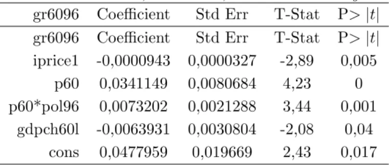
gr6095_i= b1+ b2 iprice1i+ b3 p60i+ b4 (p60 ∗ inst96)i+ b5 gdpch60li+ εi (4)

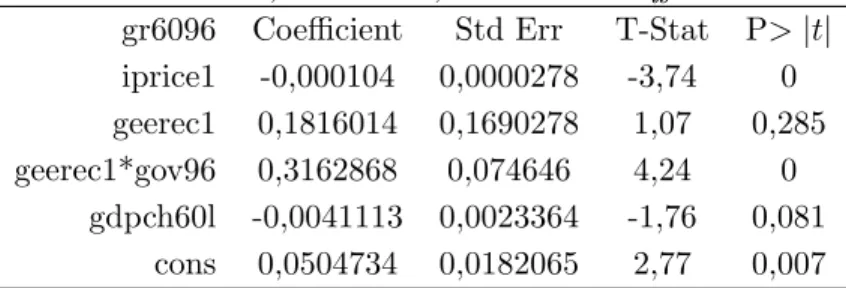
gr6095_i= b1+b2 iprice1i+b3 geerec1i+b4 (geerec1∗inst96)i+b5 gdpch60li+εi

(5) The value of each indicator2 varies from -2.5 to 2.5, an higher value indicating a better institutional situation. Corruption has many definitions, which can be related to those indicators. According to Ritva Reinikka and Jakob Svensson

(14)

(2005), corruption is defined as the lack of information and transparency in delivering education services. The lack of information and transparency can be proxied by the quality of the service delivered (Gov96 ) and the quality of contract enforcement (Rul96 ). De la Croix and Delavallade (2006) emphasize how corruption can distort the composition of public spending, by favoring sec-tors where rent seeking can be achieved more easily. Government effectiveness (Gov96 ) and regulatory burden (Reg96 ) can be used for measuring the extent of this distorsion due to rent seeking and corruption. Our own definition of corruption in the previous section is the negative externality on growth, which can be explained either by the variable control of corruption (Corr96 ) or by any dimension of public and private governance in the educational system, likely to lower the quality in delivering education services.

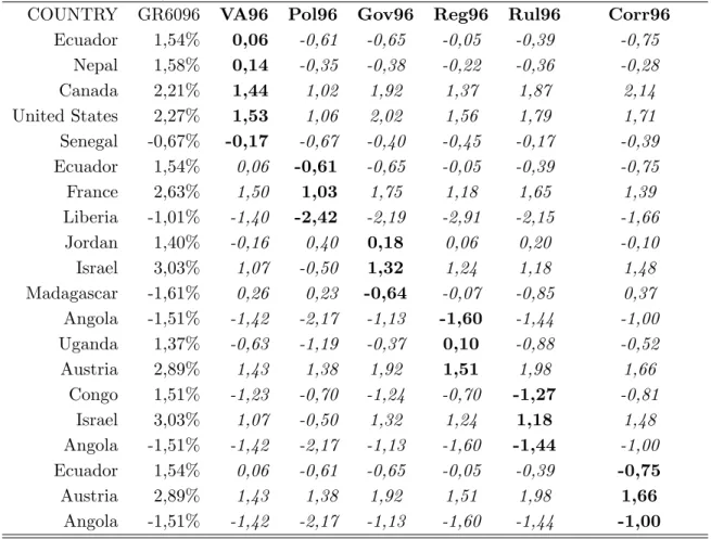
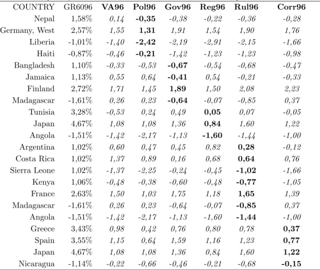
As can be seen from the interacted variables in tables 4 to 9, and tables 10 to 15, good institutions enhance growth by increasing the positive return to education (public spending on education or primary schooling). Table 1 re-ports the increase in the average rate of growth induced by an improvement in the institutional variable from its average value to the average value plus twice the standard error. All variables are taken at their mean value. Figures in the first (second) column are calculated using coefficients from equation 4 (respectively equation 5). Finally tables 2 and 3 provide cross countries com-parisons. What would have been growth in country x if the quality of a given institution had augmented by the average value plus twice the standard error, and in which developed country y do we observe the rate of growth implied by such an institutional improvement?

According to Tables 1 and 2, column A, an improvement in the Voice and Accountability variable implies an increase in the rate of growth from 1,58% -which is the rate of growth of Nepal, where the score of Voice and Accountability is relatively low (0,14) - to 2,23%, which is close to the rate of growth of Canada and that of the United States, where the scores of Voice and Accountability reflect an higher level of political, human and civil rights (respectively 1,44 and 1,53). The implied increase in growth 0,65% would have allowed Senegal to get a non-negative rate of growth. Table 1, column B, tells that an improvement in Political Instability and Violence induces an increase in growth from 1,58% (Nepal) to 2,55% (West Germany). In Nepal Political Instability is -0,35, in West Germany the score stands at 1,31. The economy of Liberia, which declined over the period at -0.87%, would have stagnated.

A better control of corruption doubles the rate of growth via a better return to education, from 1,56% to 2,92% according to equation 4 (column A in Table 1 ), and 3,56% to 4,82% according to equation 5 (column B in Table 1). Efficiently fighting against corruption would have allowed Ecuador to reach the same rate of growth as Austria (Table 2 ), and Greece or Spain to reach the same rate of

(15)

growth as Japan.

Table 1: Impact of Institutions on Growth corresponding growth computed with 4:(column A) corresponding growth computed with 5: (column B)

Institution Colunm A Colunm B Voice and Accountability

average value 1,58% 1,75%

average value plus twice the standard error 2,23% 1,75% implied increase in growth 0,65% 0,00% Political Instability and Violence

average value plus twice the standard error 2,60% 2,55% implied increase in growth 1,05% 0,97% Government Effectiveness

average value plus twice the standard error 3,02% 2,77% implied increase in growth 1,60% 1,64%

Regulatory Burden

Rule of Law

Control of Corruption

The next step of this empirical study is to instrument the institutional vari-ables for addressing the double causality running from institutions to growth and vice et versa. Variables such as the share of Protestants and former British colonies identified by Treisman (2000) are used as instruments. We use as well other variables correlated with the endogeneous explanatory variable but not with the residual of the equation, like the degree of ethnolinguistic fractional-ization, fraction buddhist, fraction catholic, landlockness, oil producing country dummy, the extent of political rights, the share of primary exports in 1970. The results are mixed, while the coefficients of either public education spending or

(16)

Table 2: Impact of Institutions on Growth: Cross countries Comparisons

COUNTRY GR6096 VA96 Pol96 Gov96 Reg96 Rul96 Corr96

Ecuador 1,54% 0,06 -0,61 -0,65 -0,05 -0,39 -0,75 Nepal 1,58% 0,14 -0,35 -0,38 -0,22 -0,36 -0,28 Canada 2,21% 1,44 1,02 1,92 1,37 1,87 2,14 United States 2,27% 1,53 1,06 2,02 1,56 1,79 1,71 Senegal -0,67% -0,17 -0,67 -0,40 -0,45 -0,17 -0,39 Ecuador 1,54% 0,06 -0,61 -0,65 -0,05 -0,39 -0,75 France 2,63% 1,50 1,03 1,75 1,18 1,65 1,39 Liberia -1,01% -1,40 -2,42 -2,19 -2,91 -2,15 -1,66 Jordan 1,40% -0,16 0,40 0,18 0,06 0,20 -0,10 Israel 3,03% 1,07 -0,50 1,32 1,24 1,18 1,48 Madagascar -1,61% 0,26 0,23 -0,64 -0,07 -0,85 0,37 Angola -1,51% -1,42 -2,17 -1,13 -1,60 -1,44 -1,00 Uganda 1,37% -0,63 -1,19 -0,37 0,10 -0,88 -0,52 Austria 2,89% 1,43 1,38 1,92 1,51 1,98 1,66 Congo 1,51% -1,23 -0,70 -1,24 -0,70 -1,27 -0,81 Israel 3,03% 1,07 -0,50 1,32 1,24 1,18 1,48 Angola -1,51% -1,42 -2,17 -1,13 -1,60 -1,44 -1,00 Ecuador 1,54% 0,06 -0,61 -0,65 -0,05 -0,39 -0,75 Austria 2,89% 1,43 1,38 1,92 1,51 1,98 1,66 Angola -1,51% -1,42 -2,17 -1,13 -1,60 -1,44 -1,00

(17)

Table 3: Impact of Institutions on Growth: Cross countries Comparisons

COUNTRY GR6096 VA96 Pol96 Gov96 Reg96 Rul96 Corr96

Nepal 1,58% 0,14 -0,35 -0,38 -0,22 -0,36 -0,28 Germany, West 2,57% 1,55 1,31 1,91 1,54 1,90 1,76 Liberia -1,01% -1,40 -2,42 -2,19 -2,91 -2,15 -1,66 Haiti -0,87% -0,46 -0,21 -1,42 -1,23 -1,23 -0,98 Bangladesh 1,10% -0,33 -0,53 -0,67 -0,54 -0,68 -0,47 Jamaica 1,13% 0,55 0,64 -0,41 0,54 -0,21 -0,33 Finland 2,72% 1,71 1,45 1,89 1,50 2,08 2,23 Madagascar -1,61% 0,26 0,23 -0,64 -0,07 -0,85 0,37 Tunisia 3,28% -0,53 0,24 0,49 0,05 0,07 -0,05 Japan 4,67% 1,08 1,08 1,36 0,84 1,60 1,22 Angola -1,51% -1,42 -2,17 -1,13 -1,60 -1,44 -1,00 Argentina 1,02% 0,60 0,47 0,45 0,82 0,28 -0,12 Costa Rica 1,02% 1,37 0,89 0,16 0,68 0,64 0,76 Sierra Leone 1,02% -1,37 -2,25 -0,24 -0,45 -1,02 -1,66 Kenya 1,06% -0,48 -0,38 -0,60 -0,48 -0,77 -1,05 France 2,63% 1,50 1,03 1,75 1,18 1,65 1,39 Madagascar -1,61% 0,26 0,23 -0,64 -0,07 -0,85 0,37 Angola -1,51% -1,42 -2,17 -1,13 -1,60 -1,44 -1,00 Greece 3,43% 0,98 0,42 0,76 0,80 0,78 0,37 Spain 3,55% 1,15 0,64 1,59 1,16 1,23 0,77 Japan 4,67% 1,08 1,08 1,36 0,84 1,60 1,22 Nicaragua -1,14% -0,22 -0,66 -0,46 -0,21 -0,68 -0,15

(18)

primary schooling in 1960 are no more significant, institutions interacted with education still matter. More importantly, the Hausman tests do not reject the null hypothesis telling that institutions are exogeneous3 . Therefore we rest on the previous results.

6 Conclusion

This paper provides an endogeneous optimal growth model for explaining the impact of corruption within the education sector. Human capital is produced through a non-linear education technology. The non-linearity is due to a fixed cost, above which investment in education yields a positive return. Below the threshold, investment in human capital does not produce any return. While a great deal of models emphasizes the consequences of corruption and more gen-erally of low quality institutions on total factor productivity, our model focuses on the effect of corruption on the return to education. Its implication is tested using the dataset collected by Xavier Sala-i-Martin, Gernot Doppelhofer, and Ronald I. Miller (2004). Empirical analysis supports the idea that corruption decreases the return to education.

References

Acemoglu D., Johnson S., Robinson, J.A., 2001. The colonial origins of com-parative development: an empirical investigation. American Economic Review 91(5), 1369-1401.

Al-Samarra Samer, 2002. Achieving education for all: how much does money matter?. IDS Working Paper 175, Institute of development Studies, Brighton, Sussex, England.

Barro, R.J., 1997. Determinants of Economic Growth.MIT Press, Cambridge.

Barro Robert, Lee Jong-Wha, 1996. Schooling Quality in a Cross Section of Countries. NBER Working Paper N 6198.

Breton R. Theodore, 2004. Can Institutions or Education explain world poverty? An augmented Solow model provides some insights. Journal of Socio-Economics, 33, 45-69.

Chua, Yvonne T., 1999. Robbed: An Investigation of Corruption in Philippine Education (Quezon City: Philippine Center for Investigative Journalism.

(19)

CIET, 1999. Corruption: The Invisible Price Tag on Education. CIET media release, October 12 (New York: CIET International).

Cockroft, Laurence, 1998. Corruption and Human Rights: A Crucial Link.TI Working Paper (Transparency International).

Corrales J, 1999. The politics of Education reform: overcoming institutional blocks. The Education Reforms and Management Series, Vol II n1, Wash-ington, D.C.: The World Bank.

De la Croix David, Delavallade, Clara, 2006, ”Growth, Public Investment and Corruption with Failing Institutions”. CORE Discussion Paper 2006/101 .

Friedman, E., Johnson S., Kaufman D., Zoidon-Lobaton, P., 2000. Dodging the grabbing hand: the determinants of unofficial activity in 69 countries. Journal of Public Economics 76, 459-493.

Greif,Avner, 1994. Individualistic Collectivist.Journal of Political Economy

Hall, R.E., Jones, C.I., 1999. Why do some countries produce so much more output per worker than others?. Quarterly Journal of Economics, 83-116. Hanusek, E.A., Kimko, D.D., 2000. Schooling, labor-force quality, and the

growth of nations. American Economic Review 5: 1184-1208.

Krueger Alan B., Lindahl Mikael, 2001. Education for Growth: Why and For Whom?. Journal of Economic Literature,Vol. XXXIX, 1101-1136.

Langseth, Peter, Stapenhurst, 1997. National Integrity System Country Stud-ies. EDI Working Paper (World Bank: Economic Development Institute.

Mankiw, N Gregory, Romer David, Weil David N., 1992. A Contribution to the Empirics of Economics Growth. Quarterly Journal of Economics, 107:2, 407-37.

North, D.C., 1990. Institutions, Institutional Change and Economic Perfor-mance. Cambridge University Press, New York.

Penrose P., 1998. Cost of Sharing in Education. London: Department for International Development.

Pritchett L., Filmer D., 1999. What Education production functions really show: a positive theory of education expenditures. Economics of Educa-tion Review, Vol 18 n2, 223-39.

(20)

Reinikka Ritva, Svensson Jakob, 2005. Fighting Corruption to Improve School-ing: Evidence from a Newspaper Campaign in Uganda. Journal of the European Economic Association, vol. 3 (2-3): 259-267.

Sala-i-Martin, Xavier, Doppelhofer Gernot, Miller Ronald I., 2004. Determi-nants of Long Term Growth: a Bayesian Averaging of Classical Estimates (BACE) Approach . American Economic Review, Vol.94, n4,.

Temple, J.R.W., 2001. Generalizations that aren’t? Evidence on education and growth. European Economic Review 45, 905-918.

Wobmann L., 2000. Schooling resources, educational institutions, and student performance: the international evidence,Kiel working paper 983. Kiel: Kiel Institute of World Economics.

(21)

Table 4: Growth, Education,Voice and Accountability gr6096 Coefficient Std Err T-Stat P> |t| iprice1 -0,0000992 0,0000341 -2,91 0,004

p60 0,0353232 0,0081749 4,32 0

p60*va96 0,004709 0,0027339 1,72 0,088 gdpch60l -0,0063468 0,0037929 -1,67 0,097 cons 0,0469749 0,0243959 1,93 0,057

Table 5: Growth, Education,Political Instability gr6096 Coefficient Std Err T-Stat P> |t| gr6096 Coefficient Std Err T-Stat P> |t| iprice1 -0,0000943 0,0000327 -2,89 0,005

p60 0,0341149 0,0080684 4,23 0

p60*pol96 0,0073202 0,0021288 3,44 0,001 gdpch60l -0,0063931 0,0030804 -2,08 0,04

cons 0,0477959 0,019669 2,43 0,017

Table 6: Growth, Education,Government Effectiveness gr6096 Coefficient Std Err T-Stat P> |t| gr6096 Coefficient Std Err T-Stat P> |t| iprice1 -0,0000814 0,0000316 -2,58 0,011

p60 0,0339602 0,008182 4,15 0

p60*gov96 0,0108602 0,0019763 5,5 0

gdpch60l -0,0107624 0,0035889 -3 0,003 cons 0,0764289 0,0225627 3,39 0,001

Table 7: Growth, Education,Regulatory Framework gr6096 Coefficient Std Err T-Stat P> |t| gr6096 Coefficient Std Err T-Stat P> |t| iprice1 -0,0000763 0,0000314 -2,43 0,017

p60 0,0321337 0,0079129 4,06 0

p60*reg96 0,0105224 0,002637 3,99 0

gdpch60l -0,0082551 0,0032012 -2,58 0,011 cons 0,0590293 0,0201235 2,93 0,004

Table 8: Growth, Education,Rule of Law gr6096 Coefficient Std Err T-Stat P> |t| gr6096 Coefficient Std Err T-Stat P> |t| iprice1 -0,0000853 0,000031 -2,76 0,007

p60 0,0352735 0,0083265 4,24 0

p60*rul96 0,0104869 0,0021306 4,92 0 gdpch60l -0,0104191 190,003617 -2,88 0,005

(22)

Table 9: Growth, Education,Corruption gr6096 Coefficient Std Err T-Stat P> |t| gr6096 Coefficient Std Err T-Stat P> |t| iprice1 -0,0000969 0,0000347 -2,79 0,006

p60 0,037631 0,0103372 3,64 0

p60*cor96 0,009314 0,0022544 4,13 0

gdpch60l -0,0108246 0,0044067 -2,46 0,016 cons 0,0771738 0,0272839 2,83 0,006

Table 10: Growth, Education,Voice and Accountability gr6096 Coefficient Std Err T-Stat P> |t| iprice1 -0,0001292 0,0000292 -4,43 0 geerec1 0,3490316 0,1867135 1,87 0,064 geerec1*va96 0,1385323 0,1002374 1,38 0,17

gdpch60l -0,000103 0,0027416 -0,04 0,97

cons 0,0211327 0,021211 1 0,321

Table 11: Growth, Education,Political Instability gr6096 Coefficient Std Err T-Stat P> |t| iprice1 -0,0001257 0,0000288 -4,36 0 geerec1 0,3336531 0,1766379 1,89 0,062 geerec1*pol96 0,1899536 0,0653656 2,91 0,004 gdpch60l 0,0001036 0,001982 0,05 0,958 cons 0,0197635 0,0154056 1,28 0,202

Table 12: Growth, Education,Government Effectiveness gr6096 Coefficient Std Err T-Stat P> |t| iprice1 -0,000104 0,0000278 -3,74 0 geerec1 0,1816014 0,1690278 1,07 0,285 geerec1*gov96 0,3162868 0,074646 4,24 0

gdpch60l -0,0041113 0,0023364 -1,76 0,081 cons 0,0504734 0,0182065 2,77 0,007

(23)

Table 13: Growth, Education,Regulatory Framework gr6096 Coefficient Std Err T-Stat P> |t| iprice1 -0,0001066 0,0000277 -3,86 0 geerec1 0,3006736 0,1621821 1,85 0,067 geerec1*reg96 0,301736 0,0693875 4,35 0

gdpch60l -0,0025102 0,0021683 -1,16 0,25 cons 0,0365615 0,0163639 2,23 0,028

Table 14: Growth, Education,Rule of Law

gr6096 Coefficient Std Err T-Stat P> |t| iprice1 -0,0001181 0,0000247 -4,79 0 geerec1 0,2317087 0,1652191 1,4 0,164 geerec1*rul96 0,3022762 0,0723724 4,18 0

gdpch60l -0,0036263 0,0022362 -1,62 0,108 cons 0,0472594 0,0173093 2,73 0,007

Table 15: Growth, Education,Corruption

gr6096 Coefficient Std Err T-Stat P> |t| iprice1 -0,0001201 0,0000308 -3,9 0 geerec1 0,2547736 0,2022274 1,26 0,211 geerec1*cor96 0,2449854 0,0845091 2,9 0,005 gdpch60l -0,0033518 0,0027593 -1,21 0,228 cons 0,0462569 0,0211743 2,18 0,031